The intrinsic dimensionality of spectro-polarimetric data

Abstract

The amount of information available in spectro-polarimetric data is estimated. To this end, the intrinsic dimensionality of the data is inferred with the aid of a recently derived estimator based on nearest-neighbor considerations and obtained applying the principle of maximum likelihood. We show in detail that the estimator correctly captures the intrinsic dimension of artificial datasets with known dimension. The effect of noise in the estimated dimension is analyzed thoroughly and we conclude that it introduces a positive bias that needs to be accounted for. Real simultaneous spectro-polarimetric observations in the visible 630 nm and the near-infrared 1.5 $\mu$m spectral regions are also investigated in detail, showing that the near-infrared dataset provides more information of the physical conditions in the solar atmosphere than the visible dataset. Finally, we demonstrate that the amount of information present in an observed dataset is a monotonically increasing function of the number of available spectral lines.

1. Introduction

High-dimensional data present difficulties when analyzing and understanding their statistical properties. The efficiency of typical statistical and computational methods usually degrades very fast when the dimensionality of the problem increases, thus making the analysis of the observed data a cumbersome or, sometimes, unfeasible task. This fact is often referred to as the curse of dimensionality. The advent of computers has permitted to face the analysis of increasingly complex data. These data usually exhibit an intricate behavior and, in order to understand the underlying physics that produces such effects, we have been forced to develop very complicated models. Ideally, these models have to be based on physical grounds but there seems to be no way of knowing in advance how complicated this model has to be to correctly reproduce the observed behavior.

In spite of their inherent complexity, the analysis of large datasets such as those produced by modern instrumentation, indicates that not all measured datapoints are equally relevant for the understanding of the underlying phenomena. In other words, it is clear that the reason why many simplified physical models are successful in reproducing a large amount of observations is because the data itself is not truly high-dimensional. Based on this premise, efforts are being made to develop methods that are capable of reducing the dimensionality of the observed datasets while still preserving their fundamental properties. Mathematically, the idea is that, while the original data may have a very large dimensionality, they are in fact confined to a small sub-region of that high-dimensional space. In this case, we can consider that the data “lives” in a subspace of low dimension (the so-called intrinsic dimension) that is embedded in the high-dimensional space. This lower dimension subspace is not usually simple to describe because it often lies in a manifold whose relation with the original high-dimensional space has to be described by a very complex non-linear (and usually unknown) function. In spite of the complexity, when facing a high-dimensionality dataset, it is of great interest to reduce the dimension of the original data prior to any modeling effort. In this manner we can uncover more easily the physics underlying the observations and even detect previously unknown properties that can be of interest.

Among the most popular methods for dimensionality reduction we find principal component analysis (PCA) or Karhunen-Loeve expansion. Due to its computational simplicity, it is one of the most widely employed methods (e.g., Rees et al., 2000; López Ariste & Casini, 2002; Socas-Navarro, 2005a; Casini et al., 2005; Ferreras et al., 2006). PCA seeks orthogonal directions in the original high-dimensional space along which the data correlation is the largest. From a computational point of view, the method finds the eigenvalues and eigenvectors of the covariance matrix obtained from a given dataset. Then, the directions on the space where the correlation is large (large eigenvalues) may be approximately described with only one parameter (a factor multiplying the associated eigenvector) and have sometimes a physical meaning. An example of this can been seen in Skumanich & López Ariste (2002), who demonstrated how the eigenvectors associated with the largest eigenvalues of the correlation matrix obtained from spectropolarimetric observations of a sunspot are related to fundamental physical parameters. They showed that the first eigenvector is associated with the average spectrum, the second eigenvector gives information about the velocity and the third eigenvector gives information about the magnetic splitting.

One of the weakest points of PCA is its linear character, because it relies only in the information provided by second order statistics. Therefore, it cannot efficiently describe a dataset whose embedding in the original high-dimensional space is a nonlinear manifold. Several methods have been developed during the last years to overcome this difficulty. Among them, we can find Locally Linear Embedding (LLE, Roweis & Saul, 2000), Isomap (Tenenbaum et al., 2000) and Self-Organizing Maps (SOM, Kohonen, 2001). These methods are very promising and have been shown to outperform PCA when reducing the dimension of datasets that present clear nonlinearities. Recently, a promising non-linear extension of PCA (kernel PCA) has also been developed (Schölkopf et al., 1998). It is based on the extension of PCA to non-linear mappings by the application of Mercer kernels and it effectively takes into account high-order statistics from the datasets. Another nonlinear version of PCA can be carried out with the aid of auto-associative neural networks (AANNs) (e.g., Socas-Navarro, 2005b, for applications in the inversion of Stokes profiles). All the previous methods are computationally expensive. AANNs require the training of a neural network with a bottleneck hidden layer that contains $d$ neurons, with $d$ the expected intrinsic dimension of the dataset. This training requires a very complex non-linear optimization that can be carried out with standard methods, such as the backpropagation algorithm (Rumelhart et al., 1986; Werbos, 1994). Concerning KPCA, it requires the numerical diagonalization of a very large correlation matrix of size $N\times N$ (Schölkopf et al., 1998). For large datasets, the diagonalization poses a heavy burden in terms of computational time and memory requirements because the correlation matrix is not sparse.

The above-mentioned tools have been introduced recently and probably require further study in order to understand all their statistical and computational properties. Unfortunately, they all suffer from a very important limitation: none of these methods is capable of giving a reliable estimation of the intrinsic dimension $d$ of the datasets. When this number is known or obtained by a different method, the previous methods are able to yield the projection of the original dataset in a nonlinear subspace of dimension $d$. If $d$ is close to the correct intrinsic dimension of the original dataset, they usually capture the structure of the nonlinear subspace and give good results. Although it seems of reduced importance, a good estimation of $d$ gives the key to understanding the physics underlying in the observations. In the framework of spectropolarimetry, it would be desirable to find possible direct relations between the nonlinear dimensions captured by these methods and the physical parameters employed for the forward modeling (magnetic field strength, filling factor, macroscopic velocities, etc.). If $d$ is too small, important features of the data are projected onto the same dimension and part of the information available is lost. If, on the contrary, $d$ is too large, then the methods can introduce noise in the nonlinear manifold. Also important is the fact that a good estimation of $d$ is very important to reduce the computational work and avoid a trial-and-error procedure.

Except for PCA and AANNs, no other dimension reduction methods have been applied to the field of spectropolarimetry. Furthermore, the authors are not aware that any nonlinear dimension reduction method has been applied to spectropolarimetric data thus far. In any case, it is always advantageous to have reliable information on the intrinsic dimensionality of the observed datasets. Although the spatial resolution of solar spectro-polarimetric observations has improved during the last decades, the resolution elements are typically much larger than the organization scales in the solar atmosphere. The ensuing mixture of signals inside the resolution element makes it necessary to use complicated models to explain the observed signals. However, it is fundamental to have in mind that too complicated models (with a large amount of free parameters) may not be constrained by the observations. This paper presents a step forward in the systematic investigation of observational datasets with the aim of extracting as much information as possible from the observations. Although we focus on spectroscopic and/or spectropolarimetric datasets, the philosophy of the approach is applicable to other kinds of data as well. Nowadays, solar spectroscopic and spectropolarimetric datasets are becoming very large and some effort is needed to correctly exploit all the information they carry about the physical processes taking place in the plasma. We review a powerful method presented recently to estimate the intrinsic dimension of a dataset and we apply it to different observations, analyzing in detail the consequences. An example of the datasets we are interested here is shown in Fig. 1. The usual intensity spectrum is shown in the upper panel for two different spectral ranges, while the wavelength variation of the circular polarization is shown in the lower panel.

2. Basic theory

2.1. Dimension estimation

The intrinsic dimension of a dataset is informally defined as the number of parameters that is needed to describe it. In other words, given a dataset consisting of $N$ different observations, each one made of an $M$-dimensional vector, we seek the dimension $m$ of the nonlinear manifold that captures the behavior of the $N$ vectors. As already stated, the dimension of this nonlinear manifold is smaller than that of the original space. This is a consequence of the large number of correlations that are present among the data. Consequently, we can consider that the number of parameters $m$ that we need to describe our observations fulfills $m\ll N$, always keeping in mind that these parameters have to be able to describe the whole nonlinear manifold.

Dimension estimation methods can be classified in two groups. The first group contains all the methods that rely on the diagonalization of a given correlation matrix (either linear, such as PCA, or nonlinear, such as kernel PCA). These methods estimate the dimension by calculating the number of eigenvalues greater than a given threshold. As discussed above, these methods depend largely on the ability to capture the nonlinearity of the manifold. Moreover, the estimated dimension critically depends on the threshold chosen, a quantity that is often difficult to define and has some degree of arbitrariness. However, model complexity information may be incorporated into the dimension estimate problem to generate a less arbitrary threshold (Asensio Ramos, 2006).

The second group contains methods based on geometry, especially important in determining the fractal dimension of dynamical systems. The analysis of dynamical systems reveals that a large fraction of them exhibit trajectories in the phase space that have not an integer dimension. After Mandelbrot (1982), these objects have been named fractals. Powerful method have been developed to estimate fractal dimensions. Many of them are based on the box-counting dimension (e.g., Kolmogorov, 1958; Hilborn, 2000). This method estimates the dimension of a given dataset by calculating the minimum number of “boxes” of side $r$ that are needed to cover the space occupied by the dataset. It is expected that the number of boxes $N(r)$ increases when $r$ decreases, so that the box-counting dimension of the dataset is given by the following scaling relation:

$$N(r)=\lim_{r\to 0}kr^{-m},$$ (1)

where $k$ is a constant. From this, the dimension is obtained by taking logarithms:

$$m=-\lim_{r\to 0}\frac{\log N(r)}{\log r}.$$ (2)

For the case of simple low dimensionality datasets, it is easy to verify that the box-counting dimension gives the correct answer. For instance, if our data are distributed on a straight line of length $L$ in a two-dimensional space, it is easy to demonstrate that $N(r)=L/r$, so that $m=1$. However, this estimation based on box-counting suffers from computational problems for complex dataset and the computational work grows exponentially with the dimension of the original data. Another less computationally intensive dimension estimation method (and probably the most popular thus far) was introduced by Grassberger & Procaccia (1983) and employs the correlation dimension. This correlation dimension is based on the observation that in a $N$-dimensional dataset, the number of pairs of points that are closer than a distance $r$ is proportional to $r^{m}$, where $m$ is the correlation dimension. Refinements to this method have been introduced recently to overcome some of its limitations (Camastra & Vinciarelli, 2002; Kégl, 2002).

2.2. Maximum likelihood dimension estimation

A recent approach to the estimation of dimension has been suggested by Levina & Bickel (2005). It has been obtained by applying the principle of maximum likelihood to the nearest neighbor distances, resulting in a method for dimension estimation that ourperforms the previous ones. Let $\mathbf{x}_{i}$ represent one of the $N$ $M$-dimensional vectors that constitute the observed dataset. The maximum likelihood dimension estimation assumes that the data points surrounding $\mathbf{x}_{i}$ can be correctly described with a uniform probability distribution function. As a consequence, the nearest neighbor distances follow a Poisson process. This also leads to an easy calculation of the statistical properties of the estimator. We assume that the observed dataset represents a nonlinear embedding of a lower dimensional space of dimension $m\ll M$. Levina & Bickel (2005) demonstrated that the maximum likelihood estimator $\hat{m}$ of the intrinsic dimension (MLEID) can be written as:

$$\hat{m}_{k}(\mathbf{x}_{i})^{-1}=\frac{1}{k-2}\sum_{j=1}^{k-1}\log\frac{T_{k}(\mathbf{x}_{i})}{T_{j}(\mathbf{x}_{i})},$$ (3)

where $T_{k}(\mathbf{x}_{i})$ represents the Euclidean distance between point $\mathbf{x}_{i}$ and its $k$-th nearest neighbor. Note that the previous equation is only valid for $k>2$.

The outcome of the previous equation depends critically on the number of neighbors $k$ that are taken into account. The reason for this is that $k$ sets the scale at which we are analyzing the dataset, and it is possible that the data have a different dimension at different scales. For instance, this is the case for a set of points in a two-dimensional space distributed according to a gaussian density. At very small scale (small value of $k$), we see individual points and the dimension is close to 0. At larger scales, the dimension reaches the value of 2 (e.g., Kégl, 2002). Like other methods, the quality of the estimated dimension usually degrades when $k$ increases as a consequence of the finite number of observations in the dataset (Levina & Bickel, 2005).

The previous equation is interesting because it allows us to give local estimations of the intrinsic dimension, in cases where one expects it to change from point to point. Although more work needs to be done, in principle it permits to locate points in the dataset that present anomalies with respect to the average behavior. In any case, it is important to take into account that large fluctuations can be expected in the estimation of the local dimension and the information provided by Eq. (3) has to be analyzed with care. However, if we assume that the observed dataset belongs to the same manifold, it is more convenient to use an estimation that takes into account all the points in the dataset. Levina & Bickel (2005) propose to use the following estimation:

$$\hat{m}_{k}=\frac{1}{N}\sum_{i=1}^{N}\hat{m}_{k}(\mathbf{x}_{i}),$$ (4)

which is simply an average over the complete dataset. On the contrary, it has been suggested elsewhere that, due to the mathematical structure of Eq. (3), it makes more sense and is more stable to carry out the average of the inverse of the estimators:

$$\hat{m}_{k}^{-1}=\frac{1}{N(k-1)}\sum_{i=1}^{N}\sum_{j=1}^{k-1}\log\frac{T_{k}(\mathbf{x}_{i})}{T_{j}(\mathbf{x}_{i})},$$ (5)

so that the estimation of the dimension is given by $1/\hat{m}_{k}^{-1}$. We have verified that both estimates give almost the same value for the dimension, although the latter has a better behavior for small values of $k$.

The computational cost of this method (Levina & Bickel, 2005) is mainly dominated by the calculation of the $k$ nearest neighbors for every point $\mathbf{x}_{i}$. The computational cost of evaluating Eqs. (4) or (5) turns out to be almost negligible. Since we are not dealing with too large datasets, our calculations rely on the calculation of the distances among all the points, so that the computational work is essentially proportional to $N^{2}$. However, alternative ways of calculating (exact or approximate) nearest neighbors have been developed, the majority of them being based on the construction of efficient tree-like structures that highly reduce the computational work.

3. Artificial datasets

3.1. Cases with a known number of dimensions

In order to show the reliability of the method introduced by Levina & Bickel (2005), it is of interest to test it with datasets of known low dimensionality. Although these tests present nothing new with respect to what is already known (e.g., Levina & Bickel, 2005, and references therein), we consider them necessary to indicate the potential of these methods. To this aim, we selected a particular Stokes $I$ profile observed with the Tenerife Infrared Polarimeter (Martínez Pillet et al., 1999) of an internetwork region of the quiet Sun (Martínez González et al., 2006a). With this profile we generate a dataset of 2000 elements by performing a random horizontal (i.e., in the wavelength direction) shift. The values of the shift obey a gaussian distribution. The estimated dimension is shown in the left panel of Fig 2. Due to the possible variation of the dimension with the scale at which the data are analyzed, we plot the estimated dimension for each value of $k$. When $k$ is small, we are referring to small scales while the scale increases when $k$ increases. Because the dataset is probably not dense enough to correctly sample the whole nonlinear manifold, there may be a systematic deviation from the correct dimension for large values of $k$. The solid line presents the estimation of the intrinsic dimension obtained from Eq. (4) while the dashed line presents the estimation given by Eq. (5). Note that they both yield similar values for the dimension, which is actually the correct one (since we have allowed only one degree of freedom). The method has captured the fact that, although these profiles are discretized in $M=231$ wavelength points, only one parameter suffices to describe the entire dataset.

A further complication is introduced in the artificial dataset by carrying out an additional vertical shift to the Stokes $I$ profile. The shift follows again a gaussian distribution that is no correlated with the horizontal shift. The estimated dimension is shown in the right panel of Fig 2. The method correctly gives a dimension of 2. Interestingly, when the vertical and horizontal shifts are forced to be correlated (for instance, we make them equal) the estimated dimension is again 1, just as one would expect.

3.2. Pure noise

Noise turns out to be a problem for estimating dimensions. If a dataset is confined inside a manifold of a high-dimensional space, the inclusion of noise tends to spread the points out of this manifold and starts to fill up a larger volume of the original high-dimensional space. Consequently, we expect that the addition of noise will tend to increase the estimated dimension asymptotically approaching $M$, the dimension of the original space. We have generated various sets of profiles with different sizes. Each profile consists of a vector of dimension $M$ made of completely uncorrelated noise following a gaussian distribution. The intrinsic dimension of a dataset composed of $M$-dimensional elements of pure noise is equal to $M$ and we expect the estimators given by Eqs. (4) and (5) to converge to this value for sufficiently large values of the number of observables $N$. The estimated dimensions for each value of $M$ are shown in Fig 3 for datasets of different sizes, from $N=500$ to $N=4000$. In order to minimize figure cluttering, the curves correspond only to the estimation given by Eq. (5). The same overall pattern is found for Eq. (4), with a behavior similar to that found in Fig 2. When $M$ is small (for instance the case with $M=10$ at the top left panel), the estimated dimension is very good for small values of $k$. It degrades as $k$ increases because the assumption of uniform distribution of the datapoints breaks for this 10-dimensional space with such a small number of points. Consequently, the assumptions under which the formalism of Levina & Bickel (2005) has been developed are not fulfilled and it cannot be applied. However, it is surprising that it is possible to have a rough estimate with a dataset of only $N=500$ elements. When the number of elements of the dataset increases, the curves asymptotically tend to $M$. For increasing values of $M$, the dimension estimate is biased towards smaller values, although it is clear that it still yields a reasonable approximation to the correct value even for very small datasets. Figure 3 shows in detail how increasing the number of elements in the dataset leads to an improved estimation of the intrinsic dimension. In the limiting case of a space with extremely large dimension ($M=230$), the method underestimates the dimension by a factor of $\sim$3.

3.3. Fe I database

One of the fastest techniques for Stokes profiles inversion is based on a look-up algorithm with PCA coefficients (Rees et al., 2000). Once a model atmosphere (with a given number of parameters) is selected, a database of models and emerging profiles is generated. The database has to be able to correctly sample the space spanned by all the parameters. Due to computational limitations, the PCA inversion technique has only been applied to the simple Milne-Eddington atmosphere thus far. The eigenvectors of the PCA decomposition are then saved, along with the projection of each element of the database on these eigenvectors, and the Milne-Eddington parameters associated with each one. In the inversion process, an observed set of Stokes profiles is projected on the eigenvectors and the corresponding projections are compared to those saved in the database. Here we have used the PCA database as our observed dataset. We are interested in estimating the dimension of the manifold in which these observation “live”. In principle, each profile contains 180 wavelength points and the phase space would have dimension 180. However, correlations between many of these wavelength points (for instance, all the continuum points that always present the same value) drastically reduce the dimension of the manifold.

The database that we use consists of $\sim$6200 solar Stokes profiles of the 6301-6302 Å region, where two Fe I lines and two telluric lines are visible. Fig 4 shows the estimated dimension for the Stokes $I$ (upper panel) and the Stokes $V$ profiles (lower panel). The database is reconstructed from the PCA eigenvectors and the projections of each element of the database on these eigenvectors. In order to see the information carried out by the eigenvectors, we show in Fig 4 the estimated dimension using an increasing number of eigenvectors $N_{\mathrm{PCA}}$ in the reconstruction. The trend obtained is very instructive, showing that the estimated dimension increases with $N_{\mathrm{PCA}}$ until a saturation is reached. The case $N_{\mathrm{PCA}}=2$ demonstrates that the first two eigenvectors contain a large amount of information and they may be seen, as shown by Skumanich & López Ariste (2002), as directly associated with physical parameters. The situation remains unchanged when reconstructing with $N_{\mathrm{PCA}}=4$ eigenvectors, while a saturation is reached when reconstructing with $N_{\mathrm{PCA}}=10$. This means that, although the number of Milne-Eddington parameters defining each element of the dataset is 9, only 6 are actually needed to describe the entire dataset. This is an alternative way of showing the strong degeneracy present in the 6301-6302 Å Fe I lines (Martínez González et al., 2006a, b). Although PCA cannot capture the possible nonlinearity of the 6-dimensional manifold, it can be shown that the first 6 eigenvectors are sufficient to describe all the elements of the database with a very small error.

3.4. The effect of noise

We have shown that the method developed by Levina & Bickel (2005) correctly captures the dimension of pure noise data. It is even more important to see how the method behaves when data is corrupted with noise. It is expected that, since the noise reduces the correlation between some of the components of the $M$-dimensional vectors that represent the dataset, the estimated dimension will grow when the signal-to-noise ratio decreases. A fundamental problem arises because it is very difficult to recognize truly high-dimensional data from low signal-to-noise data. This test has been carried out with the Fe I dataset reconstructed using all the information available (we used the first 10 eigenprofiles). We have calculated the estimated dimension for four different noise levels, given in terms of the standard deviation $\sigma$ of the gaussian noise in units of the continuum intensity. Since the typical Stokes $V$ signals are around 1-2 orders of magnitude smaller than Stokes $I$, a noise of the same $\sigma$ implies a much smaller signal-to-noise ratio for Stokes $V$ than for Stokes $I$. Consequently, we expect the dimension increase to start at smaller values of $\sigma$ for Stokes $V$ than for Stokes $I$. Figure 5 presents the results for three different values of the noise. The value of $\sigma=10^{-4}$ is small enough so that no appreciable difference is found in either Stokes $I$ or $V$ in the estimated dimension with respect to the case with no noise. When the noise increases to $\sigma=10^{-3}$, the Stokes $I$ profiles still maintain the original dimension while the estimated dimension for the Stokes $V$ dataset increases rapidly. It is interesting to note that the estimated dimension increases faster for small values of $k$. This is because the noise is small enough to produce perturbations (cancellation of correlation between the $M$ components of each Stokes profile) at very small scales, while the large scale dimension still remains unchanged. When the noise is increased further, a drastic increase of the dimension is observed in Stokes $V$ and a smaller one for Stokes $I$. Note that for even smaller signal-to-noise ratios, the estimated dimensions for large values of $k$ would also increase until reaching (in the limiting case of an infinitely large dataset) a flat dimension estimate, constant for all scales, and equal to $M$. The typical noise in spectro-polarimetric observations is usually well below 10^-3, so that it is apparent from Fig 5 that noise is not expected to change appreciably the dimensionality of noiseless data.

A consequence of the previous analysis is a possible technique to recognize when data is affected in an important manner by noise. Our datasets usually present a large value of $M$ so that, in the case of very large noise, the dimension has to grow until reaching a very large value. A clear effect of the noise, as stated in section 3.2, is that the estimated dimension rapidly increases at small values of $k$ while being held constant for large values of $k$. Thus, if a calculation shows a estimated dimension that exhibits large values at small $k$ and a steep logarithmic fall for large $k$, noise is likely rather important. A caveat is mandatory. This test relies on the behavior of the MLEID for large values of $k$. As already pointed out by Levina & Bickel (2005) and also shown here, a degradation of the dimension estimation occurs for large values of $k$ and the maximum likelihood estimation does not hold. For this reason, one has to be cautious with low signal-to-noise ratio observations. Recently, Levina et al. (2006) have addressed the problem of dimension estimation of high-noise observations when using the MLEID. Their approach to the problem is based on a smoothing of the original dataset, so that the performance of the method is greatly enhanced. They find that the estimated dimension for high-noise spectroscopic observations of chemical mixtures turns out to be extremely large. However, when a certain amount of smoothing is introduced, the MLEID turns out to be a very accurate estimation of the dimension. Thanks to the low noise in our observations, our estimations of the intrinsic dimension are surely not dominated by noise and we consider that smoothing is not necessary.

4. Observed datasets

We have shown how the MLEID developed by Levina & Bickel (2005) works for synthetic data. In this section we focus on real spectropolarimetric observations. Our aim is to learn about the intrinsic information content of the data. This may help understand how much complexity can be introduced in the models used to interpret the observational data. A proposed physical model usually consists of a set of free parameters that we have to constrain with the observations. It is crucial to have as much information as possible in the observed dataset so that one can constrain the model parameters. Obviously, it is undesirable to use too complex models to infer physical information from a dataset if the observables contain only a small amount of information. The parameters used in the physical models are typically non-orthogonal and they usually present degeneracies because the same observable can be obtained with different sets (finite or infinite) of model parameters. Although it is not straightforward to estimate from the intrinsic dimension how many parameters one can introduce in the modeling, it obviously should not be much larger than the estimated intrinsic dimension. If this number is made much larger, many of these parameters may not be constrained by the observations, thus leading to unphysical results or ill-conditioned inversions.

An important application of the estimated dimension tools we have presented here is to make relative comparisons of the intrinsic information present in two different observations. There is an ongoing debate about the different results obtained for unresolved magnetic fields in the quiet Sun from the inversion of two pairs of Fe I lines at two different spectral regions, one at 6302 Å and the other one at 1.56 $\mu$m. Recently, Martínez González et al. (2006b) has demonstrated that the information available in the pair of lines at 6302 Å is not sufficient to constrain simultaneously the intrinsic magnetic field strength and the thermodynamical properties of the plasma. They showed that it is possible to obtain exactly the same observables from completely different combinations of model parameters. Here, we consider this problem by analyzing in detail the amount of information available in the two different spectral regions. To this aim, we compare the intrinsic dimension of the two pairs of Fe I lines.

The observations employed here have been explained in detail elsewhere (Martínez González et al., 2006a, c) and an example has been already shown in Fig. 1. They were targeted to the detailed investigation of the magnetic properties of internetwork regions in the quiet Sun. These high spatial resolution observation were taken simultaneously at two different spectral windows, one in the visible around 6302 Å and the other one in the near-IR around 1.56 $\mu$m. The visible observations were acquired with the Polarimetric Littrow Spectrograph (POLIS; Beck et al., 2005) while the near-IR data were obtained with the Tenerife Infrared Polarimeter (TIP; Martínez Pillet et al., 1999). Both instruments were mounted at the German Vacuum Tower Telescope (VTT), located at the Observatorio del Teide of the Instituto de Astrofísica de Canarias. The instruments were used in a configuration such that simultaneous and co-spatial observations of the same field-of-view were possible. The noise level for both sets of data is of the order of 5$\times$10^-5 in units of the continuum intensity.

The Stokes profiles at each spatial location were considered as vectors in a space of dimension $M=240$. In principle, one expects that, unless noise dominates the signal, the intrinsic dimension has to be much smaller than $M$. This follows from the fact that simple physical models are successful in reproducing many of the properties of the observed Stokes profiles. In fact, this is the case as shown in Fig 6. The figure shows the estimated dimension of the observed dataset, the upper panel displaying the results for the TIP observations and the lower panel presenting the POLIS results. The intrinsic dimension has been estimated for Stokes $I$ and $V$ separately using a database of 5000 observed profiles. The results obtained with Eq. (4) are in solid line and those of Eq. (5) are in dashed line. It is clear from the figure that the intrinsic dimension of Stokes $I$ is always smaller than for Stokes $V$, implying that the amount of information encoded in the Stokes $I$ profiles is smaller than that in the circular polarization profiles. The magnetic field in these observations is unresolved and the filling factor of the magnetic regions inside the resolution element is of the order of 2%. Therefore, the Stokes $I$ profile is representative of the 98% of the resolution element that is non-magnetic and carries virtually no information about the magnetic field. One expects that it may contain information about the Doppler velocity shift, temperature and density stratifications.

Focusing on Stokes $I$, we can see that the estimated dimension is very stable with respect to the scale at which the data are observed. According to the previous discussions, there is no indication of an artificial increase of the dimension due to noise, as expected for these low-noise observations. The presence of noise tends to raise the dimension for small values of $k$, also increasing the slope of the curve for larger values of $k$. It is interesting to point out that the curve obtained for the dataset in the visible spectral range appears to be more stable with $k$ than that for the near-IR lines. This indicates that the near-IR data present a richer structure, also yielding a structure that changes with the scale at which one analyzes it. It is not obvious to build up an intuitive idea of what this variation means. A possible interpretation might be that the set of similar Stokes $I$ profiles present a small variability (dimension $\sim$3), thus it is possible to describe them with a very reduced set of parameters. It is plausible to consider that similar Stokes $I$ profiles are also observed in nearby spatial locations or locations exhibiting similar brightness (bright granules versus dark lanes). This result might appear obvious because data seen at small scale typically appear similar unless strong pixel-to-pixel variations are present in the observations. When the scale is increased, the variability increases as well (dimension $\sim$6), meaning that the set of parameters used for describing them would need to be augmented. In these intermediate values of $k$, we are focusing on the differences between Stokes $I$ profiles coming from different regions (granules and lanes). Therefore, the lack of variation of the visible data has important consequences, in the sense that their Stokes $I$ profiles tend to be less sensitive to the physical properties of the atmosphere. When the data are observed at large scale, the behavior of both spectral domains tends to be similar. The decay for $k\gtrsim 1000$ is likely produced by the breakage of the fundamental assumption that the points follow a uniform distribution in the neighborhood of every point. The conclusion from the results obtained for Stokes $I$ is that there seems to be an indication that the near-IR data are capable of detecting more variability in the observations than the visible data.

Turning our attention to Stokes $V$, essentially the same behavior is observed with almost invariable estimated dimensions for the visible data and strong variations for the near-IR data. The estimated dimension is $\sim$10 for the visible data and only for $k\gtrsim 1000$ we detect a drop-off. From the results shown in Fig 6 it is clear that the near-IR data capture more physical information about the atmosphere where they are formed. This is another way of looking at the issues described by (Martínez González et al., 2006b). Among other problems, due to the small splitting present in the visible lines, it is possible to mask variations in the magnetic field as variations in the thermodynamical parameters. Consequently, these parameters alone are not constrained by the observations and only some (possibly nonlinear) combination of them can be constrained. The splitting in the near-IR lines is much larger (the splitting is proportional to the wavelength and the effective Landé factor) and these problems are less prominent. On the other hand, the visible lines produce much stronger signals and are less sensitive to noise, especially for weak ($\lesssim$500 G) fields.

5. Augmenting information

We have already pointed out that the information encoded in the pair of lines at 6302 Å is not sufficient to constrain simultaneously the thermodynamical and magnetic properties of the plasma in small unresolved magnetic structures in the quiet Sun. It has been suggested that the solution to this problem relies on the simultaneous observation of many spectral lines (e.g., Semel, 1981; Socas-Navarro, 2004). Each line contributes by adding somewhat different (hopefully complementary) information and constraints, so that the thermodynamical and magnetic properties of the plasma can be inferred with more confidence. This increase in the information content must be accompanied by an increase in the intrinsic dimension of the space spanned by the observations. It is likely that a large fraction of the information carried out by all the spectral lines is common and only a small part can be better inferred from a set of lines. Consequently, it is expected that the inclusion of each additional spectral line would increase slightly the information available, unless the new line turns out to be sensitive to a physical parameter to which the original set was nearly insensitive. In order to investigate this in detail, we show in Fig 7 the intrinsic dimension obtained using Eq. (5) for three synthetic datasets. These datasets contain the pair of Fe I lines at 1.56 $\mu$m, the pair of Fe I lines at 6302 Å and the Mn I line at 8740Å. The full dataset has been obtained using Local Thermodynamical Equilibrium (LTE) synthetic profiles. The HSRA model atmosphere (Gingerich et al., 1971) was chosen as a reference and random values of the following nine parameters were added to it, producing 10000 different random profiles: macro- and micro-turbulent velocities, filling factor, temperature offset (shifting the whole HSRA temperature height profile), temperature gradient (changing the slope of the reference temperature height profile), magnetic field offset, magnetic field gradient, velocity field offset and velocity gradient. A total of 9 parameters have been used to construct the database. If the lines contain reliable information about the 9 parameters, one would expect to infer an intrinsic dimension close to 9. However, this is not the case, as can be seen in Fig 7. The maximum value of the dimension we obtain is only 6 and this is the maximum number of orthogonal parameters we can introduce in our modeling. There are two possible reasons for this. First, the parameters we have varied for generating the database might be degenerate, in the sense that (possibly nonlinear) combinations of two or more parameters yield the same (or very similar) emergent profiles. Second, it is possible that some information be lost in the line formation process due to radiative transfer effects (e.g., line-of-sight blurring). Both mechanisms tend to reduce the information available in the observations.

A very important conclusion of this synthetic experiment is that the amount of information that we can extract from a set of observables increases with the number of spectral lines included in the set increases. This might sound obvious, but our approach of calculating the intrinsic dimensionality of the observed dataset demonstrates this point rigorously for the first time. The increase in the information content is shown in Fig 7, where we have plotted the intrinsic dimension obtained from the considered lines. We have also overplotted the result that we obtain when the intrinsic dimension is estimated considering all the lines simultaneously. Fig 7 demonstrates that the available information is a monotonically increasing function of the number of lines.

It is important to note, however, that the results presented in this section are not in accordance with those shown in the previous section. In the synthetic experiment carried out here, the 630 nm lines capture slightly more information than the 1.5 $\mu$m. We assign this apparently puzzling behavior to the fact that this synthetic test is not realistic in the sense that either the variations in the physical properties that we have included are not representative of what is happening in the solar atmosphere, either that the solar case contains correlations among physical parameters absent from the database, or both.

6. Conclusions

We have applied a computationally efficient method developed by Levina & Bickel (2005) for estimating the intrinsic dimension of a dataset. The method relies only on the calculation of the euclidean distances between the observables (taken as vectors in a high-dimensional space). The properties of the method have been analyzed in detail with artificial datasets. We have verified that it is able to correctly estimate the intrinsic dimension in artificially generated data. If the simulated observations contain noise, the method correctly estimates an increase in the intrinsic dimension that tends towards the dimension of the high-dimensional space. In very high-dimensional spaces with a small number of observations, the assumptions under which the method relies are not fulfilled, so that the method cannot be applied. The presence of noise in the observations produces an overestimation of the dimension at small values of $k$ and it may be used to judge whether the information has been significantly degraded by the presence of noise. Since both an intrinsically high-dimensional manifold and the noise produce an increase in the estimated dimension, it turns out to be extremely difficult to discriminate between both. We have suggested a possible way of discriminating both effects by analyzing the behavior of the MLEID curve for large values of $k$. However, it suffers from problems because the hypotheses under which MLEID is based are not correctly fulfilled for large values of $k$. The application of the method to real observations in the pair of Fe I lines at 1.56 $\mu$m and the pair at 6302 Å shows that the near-IR lines appear to carry more information than the visible ones. An extra numerical experiment has shown unequivocally that the amount of information that may be obtained from an observed dataset increases as the number of included lines increases.

Although this work has focused on spectro-polarimetric datasets, it is fundamental to point out the enormous applicability of the estimators of the intrinsic dimension like the one presented by Levina & Bickel (2005). Physics, and specially Astrophysics depends on the development of models with different levels of complexity that are used to explain the observables. A posteriori, inversion techniques allow to infer the properties of the object under study by fitting the observables with the proposed model. The complexity of the model has to be constrained by the amount of information available in the observables. Consequently, the estimators of the intrinsic dimensionality of the observed datasets help us accept or reject different models depending on the amount of information carried out by the observables.

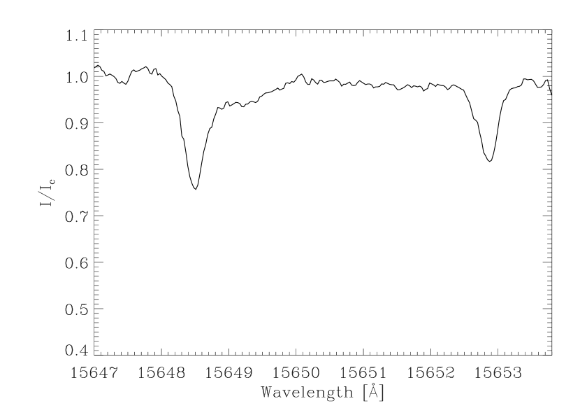
Figure 1.— Example of the spectropolarimetric data that we have analyzed in this work. These observations have been obtained in an internetwork region of the quiet Sun (Martínez González et al., 2006a, c). The upper panel shows the Stokes $I$ profiles in two different spectral regions, one in the near-IR and the other in the visible. The lower panel shows the circular polarization Stokes $V$ profiles.

Figure 2.— Estimated dimension for two simple cases. In the left panel we show the result when the database consists of a single profile that is horizontally shifted by a random sub-pixel quantity. The method correctly yields a value of 1 for the dimension. The right panel shows the result when an additional vertical shift is applied, giving the correct value of 2.

Figure 3.— Estimated dimension for profiles composed of noise. The number of wavelength points considered in each case is shown in the title.

Figure 4.— Estimated dimension for the Stokes I and V database of Fe I as different numbers of PCA components are used in the reconstruction.

Figure 5.— Effect of noise on the estimated dimension of the synthetic Fe I dataset. The dimension increases with increasing noise, with Stokes $V$ more sensitive than Stokes $I$ due to the difference in amplitude. The noise amplitude $\sigma$ is given in terms of the continuum intensity.

Figure 6.— Estimated dimension for Stokes $I$ (left panel) and Stokes $V$ (right panel) profiles of the 15648-15652 Å region observed with TIP. The large increase of the dimension for Stokes $V$ might be associated with the larger noise with respect to the noise present in the Stokes $I$ profiles. Estimated dimension for Stokes $I$ (left panel) and Stokes $V$ (right panel) profiles of the 6301-6302 Å region observed with POLIS.

Figure 7.— Synthetic test that shows how the information encoded in the observations increase when the number of spectral lines increases. The estimated intrinsic dimension is shown for Stokes $I$ (left panel) and for Stokes $V$ (right panel) for a synthetic dataset (see text for details). The intrinsic dimension is a monotonically increasing function of the number of lines included in the dataset.

References

- Asensio Ramos (2006) Asensio Ramos, A. 2006, ApJ, 646, 1445
- Beck et al. (2005) Beck, C., Schmidt, W., Kentischer, T., & Elmore, D. 2005, A&A, 437, 1159
- Camastra & Vinciarelli (2002) Camastra, F., & Vinciarelli, A. 2002, IEEE Trans. on Pattern Analysis and Machine Intelligence, 24, 1404
- Casini et al. (2005) Casini, R., Bevilacqua, R., & López Ariste, A. 2005, ApJ, 622, 1265
- Ferreras et al. (2006) Ferreras, I., Pasquali, A., de Carvalho, R. R., de la Rosa, I. G., & Lahav, O. 2006, MNRAS, 616
- Gingerich et al. (1971) Gingerich, O., Noyes, R. W., Kalkofen, W., & Cuny, Y. 1971, Sol. Phys., 18, 347
- Grassberger & Procaccia (1983) Grassberger, P., & Procaccia, I. 1983, Physica D, 9, 189
- Hilborn (2000) Hilborn, R. C. 2000, Chaos and Nonlinear Dynamics, 2nd Edition (New York: Oxford University Press)
- Kégl (2002) Kégl, B. 2002, Advances in NIPS, 14, 1404
- Kohonen (2001) Kohonen, T. 2001, Self-organizing maps (Berlin: Springer)
- Kolmogorov (1958) Kolmogorov, A. N. 1958, Dokl. Akad. Nauk. SSSR, 119, 861
- Levina & Bickel (2005) Levina, E., & Bickel, P. J. 2005, in Advances in NIPS, Vol. 17
- Levina et al. (2006) Levina, E., Wagaman, A. S., Callender, A. F., Mandair, G. S., & Morris, M. D. 2006, J. Chemom., in press
- López Ariste & Casini (2002) López Ariste, A., & Casini, R. 2002, ApJ, 575, 529
- Mandelbrot (1982) Mandelbrot, B. B. 1982, The Fractal Geometry of Nature (San Francisco: W. H. Freeman)
- Martínez González et al. (2006a) Martínez González, M. J., Collados, M., & Ruiz Cobo, B. 2006a, in Solar Polarization 4, ed. R. Casini & B. W. Lites, ASP Conf. Ser., in press
- Martínez González et al. (2006b) Martínez González, M. J., Collados, M., & Ruiz Cobo, B. 2006b, A&A, 456, 1159
- Martínez González et al. (2006c) Martínez González, M. J., Collados, M., Ruiz Cobo, B., & Beck, C. 2006c, ApJ, in preparation
- Martínez Pillet et al. (1999) Martínez Pillet, V., Collados, M., Bellot Rubio, L. R., Rodríguez Hidalgo, I., Ruiz Cobo, B., & Soltau, D. 1999, in Astronomische Gesselschaft Meeting Abstracts, vol. 15
- Rees et al. (2000) Rees, D. E., López Ariste, A., Thatcher, J., & Semel, M. 2000, A&A, 355, 759
- Roweis & Saul (2000) Roweis, S., & Saul, L. K. 2000, Science, 290, 2323
- Rumelhart et al. (1986) Rumelhart, D., Hinton, G., & Williams, R. 1986, in Parallel Distributed Processing: Explorations in the Microstructure of Cognition, ed. D. Rumelhart & J. McClelland (Cambridge: MIT), 318
- Schölkopf et al. (1998) Schölkopf, B., Smola, A. J., & Müller, K.-R. 1998, Neural Computation, 10, 1299
- Semel (1981) Semel, M. 1981, A&A, 97, 75
- Skumanich & López Ariste (2002) Skumanich, A., & López Ariste, A. 2002, ApJ, 570, 379
- Socas-Navarro (2004) Socas-Navarro, H. 2004, ApJ, 613, 610
- Socas-Navarro (2005a) —. 2005a, ApJ, 620, 517
- Socas-Navarro (2005b) —. 2005b, ApJ, 621, 545
- Tenenbaum et al. (2000) Tenenbaum, J. B., de Silva, V., & Langford, J. C. 2000, Science, 290, 2319
- Werbos (1994) Werbos, P. 1994, The Roots of Backpropagation: From Ordered Derivatives to Neural Networks and Political Forecasting (New York: John Wiley & Sons)