The Sloan Lens ACS Survey. IV: the mass density profile of early-type galaxies out to 100 effective radii

Abstract

We present a weak gravitational lensing analysis of 22 early-type (strong) lens galaxies, based on deep Hubble Space Telescope images obtained as part of the Sloan Lens ACS Survey. Using advanced techniques to control systematic uncertainties related to the variable point spread function and charge transfer efficiency of the Advanced Camera for Surveys (ACS), we show that weak lensing signal is detected out to the edge of the Wide Field Camera ($\lesssim 300\,h^{-1}\,{\rm kpc}$ at the mean lens redshift $z=0.2$). We analyze blank control fields from the COSMOS survey in the same manner, inferring that the residual systematic uncertainty in the tangential shear is less than 0.3%. A joint strong and weak lensing analysis shows that the average total mass density profile is consistent with isothermal (i.e. $\rho\propto r^{-2}$) over two decades in radius (3-300 $\,h^{-1}\,{\rm kpc}$, approximately 1-100 effective radii). This finding extends by over an order of magnitude in radius previous results, based on strong lensing and/or stellar dynamics, that luminous and dark component “conspire” to form an isothermal mass distribution. In order to disentangle the contributions of luminous and dark matter, we fit a two-component mass model (de Vaucouleurs + Navarro Frenk & White) to the weak and strong lensing constraints. It provides a good fit to the data with only two free parameters; i) the average stellar mass-to-light ratio $M_{*}/L_{V}=4.48\pm 0.46\,h{\rm M}_{\odot}/{\rm L}_{\odot}$ (at $z=0.2$), in agreement with that expected for an old stellar population; ii) the average virial mass-to-light ratio $M_{\rm vir}/L_{V}=246^{+101}_{-87}\,h{\rm M}_{\odot}/{\rm L}_{\odot}$. Taking into account the scatter in the mass-luminosity relation, this latter result is in good agreement with semi-analytical models of massive galaxies formation. The dark matter fraction inside the sphere of radius the effective radius is found to be $27\pm 4\%$. Our results are consistent with galaxy-galaxy lensing studies of early-type galaxies that are not strong lenses, in the region of overlap (30-300 $\,h^{-1}\,{\rm kpc}$). Thus, within the uncertainties, our results are representative of early-type galaxies in general.

1. Introduction

It is now commonly accepted that cold non-baryonic dark matter dominates the dynamics of the Universe. Whereas the so-called $\Lambda$CDM (cold dark matter) paradigm has been remarkably successful at reproducing with high level of precision the properties of the universe on scales larger than Mpc (e.g.  Spergel et al. 2006; Tegmark et al. 2004; Seljak et al. 2005), the situation at galactic and subgalactic scales is more uncertain. Dark-matter-only numerical simulations make very clear predictions. Dark matter halos have a characteristically “cuspy” radial profile (e.g.  Navarro et al. 1997; Moore et al. 1998; Ghigna et al. 1998; Jing 2000; Stoehr et al. 2002; Navarro et al. 2004), are triaxial (Jing 2002; Kazantzidis et al. 2004; Hayashi et al. 2006), and have abundant substructure (e.g.  Moore et al. 1999; De Lucia et al. 2004; Gao et al. 2004; Taylor & Babul 2004). From an observational point of view, substantial effort has been devoted to comparing those predictions to observations with debated results in the case e.g. of low surface brightness galaxies (Salucci 2001; de Blok et al. 2003; Swaters et al. 2003; Gentile et al. 2004; Simon et al. 2005) or at galaxy cluster scales (e.g.  Sand et al. 2004; Gavazzi 2005; Comerford et al. 2006). The main source of ambiguity in such comparisons is due to the effects of baryons. Although a minority in terms of total mass, baryons are dissipative and spatially more concentrated than the dark matter, playing a critical role at scales below tens of kiloparsecs. Understanding baryonic physics and the interplay between dark and luminous matter is necessary to understand how galaxies form and, ultimately, to test the cosmological model. From an observational point of view, measuring the relative spatial distribution of stars, gas, and dark matter is essential to provide clues to help understand the physical processes and hard numbers to perform quantitative tests of models.

The dark halos of early-type (i.e. elliptical and lenticular) galaxies have been particularly hard to detect and study, due to the general lack of kinematic tracers, such as HI, at large radii. Studies of local galaxies based on stellar kinematics (Bertin et al. 1994; Gerhard et al. 2001; Mamon & Łokas 2005a, b; Cappellari et al. 2006), kinematics of planetary nebulae (Romanowsky et al. 2003; Arnaboldi et al. 2004; Merrett et al. 2006) and temperature profile of X-ray emitting plasma (Humphrey et al. 2006) indicate that at least for the most massive systems dark matter halos are generally present. The total mass density profile is found to be close to isothermal ($\rho_{\rm tot}\propto r^{-2}$) on scales out to a few effective radii.

In the distant universe an additional mass tracer is provided by gravitational lensing. At scales comparable to the effective radius, strong gravitational lensing makes it possible to detect and study the mass profile and shape of individual halos (Kochanek 1995) or statistically of a population of halos (Rusin et al. 2003). The combination of strong lensing with stellar kinematics (Treu & Koopmans 2002; Koopmans & Treu 2002, 2003; Treu & Koopmans 2004; Koopmans et al. 2006) is particularly effective, and allows one to decompose the total mass distribution into a luminous and dark matter with good precision, yielding information on the internal structure of early-type galaxies all the way out to the most distant lenses known at $z\sim 1$. At larger scales, the surface mass density is too low to produce multiple images. However, the weak lensing signal can be detected statistically by stacking multiple galaxies and measuring the distortion of the background galaxies. The statistical nature of this measurement imposes a certain degree of spatial smoothing or binning, which in turn limits the angular resolution of weak lensing studies.

In this paper we exploit deep ACS images of 22 gravitational lenses from the Sloan Lens ACS Survey (Bolton et al. 2006; Treu et al. 2006a; Koopmans et al. 2006, hereafter papers I, II and III, respectively) to perform a joint weak and strong lensing analysis. This allows us to bridge the gap between the two regimes and study the mass density profile of early-type galaxies across the entire range $\sim$1-100 effective radii, disentangling the luminous and dark components.

From a technical point of view, joint weak and strong lensing analysis has already been applied in the past to clusters of galaxies and galaxies in clusters (Natarajan & Kneib 1997; Geiger & Schneider 1998; Natarajan et al. 2002; Kneib et al. 2003; Gavazzi et al. 2003; Bradač et al. 2005b, a). However, there are important differences with respect to galaxy scales. First and foremost, clusters produce a much stronger weak lensing signal and therefore it can be detected and studied for individual systems. Second, since clusters are spatially more extended than galaxies, relatively large smoothing scales can be adopted to average the signal over background galaxies. In contrast, the signal of individual galaxies is too “weak” to be detected, so that stacking a number of lens galaxies is required to reach a sufficient density of background sources. For this purpose, previous studies have typically relied on very large sample of galaxies (Brainerd et al. 1996; Griffiths et al. 1996; Wilson et al. 2001; Guzik & Seljak 2002; Hoekstra et al. 2004, 2005; Kleinheinrich et al. 2006) or recently in the SDSS survey (Sheldon et al. 2004; Mandelbaum et al. 2006, hereafter S04 and M06 respectively). As we will show in the rest of the paper, the high density of useful background galaxies afforded by deep ACS exposures ($\sim$72 per square arcmin) allows us to achieve a robust detection of the weak lensing signal with only 22 galaxies, and to study the mass density profile with unprecedented radial resolution.

The paper is organized as follows. After briefly summarizing the gravitational lensing formalism and notation in § 2, we discuss the sample, data reduction and analysis, and the main observational properties of the lens galaxies in § 3. § 4 details the shear measurement, with a particular emphasis on the precision correction for instrumental systematic effects and on tests of residual systematics by means of a parallel analysis of blank fields. This section also presents the mean radial shear profile around SLACS strong lenses and high resolution two-dimensional mass reconstructions. We combine strong and weak gravitational lensing constraints in § 5 to model the radial profiles lenses and disentangle the stellar and dark Matter components. We discuss our results in § 6 and give a brief summary in § 7.

Throughout this paper we assume the concordance cosmological background with $H_{0}=100\,h\,\,{\rm km\,s}^{-1}\,{\rm Mpc}^{-1}$, $\Omega_{\rm m}=0.3$ and $\Omega_{\Lambda}=0.7$. All magnitudes are expressed in the AB system.

2. Basic lensing equations

In this section we briefly summarize the necessary background of gravitational lensing and especially the weak lensing regime which concerns the present analysis. The main purpose of this section is to define notations. We refer the reader to the reviews of Mellier (1999), Bartelmann & Schneider (2001) and Schneider (2006) for more detailed accounts.

The fundamental quantity for gravitational lensing is the lens potential $\psi(\vec{\theta})$ at angular position $\vec{\theta}$ which is related to the surface mass density $\Sigma(\vec{\theta})$ projected onto the lens plane through

$$\psi(\vec{\theta})=\frac{4G}{c^{2}}\frac{D_{\rm ol}D_{\rm ls}}{D_{\rm os}}\int{\rm d}^{2}\theta^{\prime}\Sigma(\vec{\theta}^{\prime})\ln|\vec{\theta}-\vec{\theta}^{\prime}|\;,$$ (1)

where $D_{\rm ol}$, $D_{\rm os}$ and $D_{\rm ls}$ are angular distances to the lens, to the source and between the lens and the source respectively. The deflection angle $\vec{\alpha}=\vec{\nabla}\psi$ relates a point in the source plane $\vec{\beta}$ to its image(s) in the image plane $\vec{\theta}$ through the lens equation $\vec{\beta}=\vec{\theta}-\vec{\alpha}(\vec{\theta})$. The local relation between $\vec{\beta}$ and $\vec{\theta}$ is the Jacobian matrix $a_{ij}=\partial\beta_{i}/\partial\theta_{j}$

$$a_{ij}=\delta_{ij}-\psi_{,ij}=\left(\begin{array}[]{cc}1-\kappa-\gamma_{1}&-\gamma_{2}\\ -\gamma_{2}&1-\kappa+\gamma_{1}\end{array}\right)\;.$$ (2)

The convergence $\kappa(\vec{\theta})=\Sigma(\vec{\theta})/\Sigma_{\rm crit}$ is directly related to the surface mass density via the critical density

$$\Sigma_{\rm crit}=\frac{c^{2}}{4\pi G}\frac{D_{\rm os}}{D_{\rm ol}D_{\rm ls}}\;,$$ (3)

and satisfies the Poisson equation

$$\Delta\psi=\psi_{,11}+\psi_{,22}=2\kappa\;.$$ (4)

The 2-component shear is $\gamma=\gamma_{1}+i\gamma_{2}=\frac{1}{2}(\psi_{,11}-\psi_{,22})+i\psi_{,12}$ in complex notation. An elliptical object in the image plane is characterized by its complex ellipticity $e$. In the weak lensing regime, the source intrinsic ellipticity $e_{s}$ and $e$ are simply related by $e=e_{s}+\gamma$.

It is convenient to express the shear into a tangential and a curl term $\gamma=\gamma_{t}+i\gamma_{\times}$ such that $\gamma_{t}=-\mathcal{R}\left\{\gamma e^{-2i\varphi}\right\}$ and $\gamma_{\times}=-\mathcal{I}\left\{\gamma e^{-2i\varphi}\right\}$ with $\varphi$ the polar angle. For a circularly symmetric lens, $\gamma_{\times}$ vanishes whereas $\gamma_{t}$ at radius $r$ can be written as the difference between the mean convergence within that radius $\overline{\kappa}(<r)$ and the local convergence at the same radius $\kappa(r)$ :

$$\gamma_{t}=\overline{\kappa}(<r)-\kappa(r)\,.$$ (5)

In equations 1 to 5 we can isolate a geometric term which linearly scales the lensing quantities $\kappa$, $\psi$, and $\gamma$ and only depends on the distance ratio $D_{\rm ls}/D_{\rm os}$. We thus can write $\psi=w(z_{\rm l},z_{\rm s})\psi_{\infty}$ (and analogously for $\kappa$ and $\gamma$) with $w(z_{\rm l},z_{\rm s})=D_{\rm ls}/D_{\rm os}\Theta(z_{\rm s}-z_{\rm l})$, where $\Theta(x)$ is the Heaviside step function. If sources are not confined in a thin plane, we account for the distribution in redshift by defining an ensemble average distance factor $\overline{w}(z_{\rm l})$ such that:

$$\overline{w}(z_{\rm l})=\langle w(z_{\rm l},z_{\rm s})\rangle_{z_{\rm s}}=\frac{\displaystyle\int_{z_{\rm l}}^{\infty}{\rm d}z_{\rm s}\,n(z_{\rm s})\frac{D_{\rm ls}}{D_{\rm os}}}{\displaystyle\int_{0}^{\infty}{\rm d}z_{\rm s}\,n(z_{\rm s})}\,.$$ (6)

3. The data

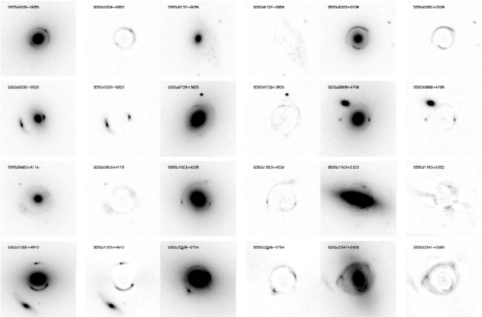
Figure 1.— F814W gallery of the 12 new SLACS lenses. The postage stamps are 7.2 arcseconds on a side. From top to bottom: SDSSJ0029-0055, SDSSJ0157-0056, SDSSJ0252+0039, SDSSJ0330-0020, SDSSJ0728+3835, SDSSJ0808+4706, SDSSJ0903+4116, SDSSJ1023+4230, SDSSJ1103+5322, SDSSJ1205+4910, SDSSJ2238-0754, and SDSSJ2341+0000. For each lens we show the original image (left) and after subtraction of a model for the lens surface brightness (right).

3.1. Lens sample

In this paper we focus on a subsample of 22 lens early-type galaxies taken from the SLACS Survey (paper I). The subsample is defined as all the confirmed lenses for which deep, 1-orbit long, ACS image through filter F814W were available as of the cutoff date for this paper, 2006 October 15. The parent sample is spectroscopically identified from the SDSS database and confirmed by ACS imaging, as described in paper I (see also Bolton et al. 2004). Ten lenses are in common with the sample previously analyzed in papers II and III, while the remaining 12 lenses were not analyzed in papers II and III. Images of the 12 new lenses are shown in Figure 1. Table 1 summarizes the most relevant properties of the 22 lenses. More details on the new lenses and on the ongoing programs will be presented elsewhere.

The SDSS aperture velocity dispersions are in the range $196\leq\sigma_{v}\leq 333\,{\rm km\,s}^{-1}$ and the mean square velocity dispersion is $\langle\sigma_{v}^{2}\rangle^{1/2}\simeq 248\,{\rm km\,s}^{-1}$. The lens galaxies have a mean redshift $\langle z_{\rm l}=0.22\rangle$. Paper II showed that SLACS strong lenses fall on the same Fundamental Plane of non-lens early-type galaxies (see also Bolton et al. 2007, in prep). This demonstrates that – within our measurement errors – lensing galaxies have normal internal dynamical properties at small scales. One of the goals of this paper is to combine strong with weak lensing to check whether the outer regions of the SLACS lenses behave in a peculiar way as compared to non-lens early-type galaxies.

3.2. HST observations & data reduction

The sample was observed with the Advanced Camera for Surveys on board HST between November 2005 and October 15 2006, as part of HST programs 10494 (PI: Koopmans) and 10886 (PI: Bolton). One-orbit exposures were obtained through filter F814W (hereafter $I$) with the Wide Field Camera centering the lens on the WFC1 aperture, i.e. in the center of the second CCD. Hence the observations cover a region as far as 3$\arcmin$ around the lenses. Four sub-exposures were obtained with a semi-integer pixel offset (acs-wfc-dither-box) to ensure proper cosmic ray removal and sampling of the point spread function. For the lenses in program 10494 additional one orbit exposures with ACS through filter F555W and with the NICMOS NIC2 camera through filter F160W are also available. In this paper, the additional F555W exposure is used to check satellite/foreground contamination to the weak-lensing catalog. A full detailed analysis of the multi-color images will be presented elsewhere.

Since the goal of this paper is detecting the weak lensing signal produced by the SLACS strong lenses, we optimize our reduction according to the prescriptions of Rhodes et al. (2007, hereafter R07). For each target, we used multidrizzle (Koekemoer et al. 2002) to combine the four subexposures, using a final pixel size of 0$\farcs$03 and a Gaussian interpolation kernel.

One important difference between this study and that of R07, is that ours are pointed observations. Thus instrumental effects could play a different role than for weak-lensing studies of objects at random positions on the detector, possibly introducing systematic errors. In order to determine the amplitude of systematic errors in our weak lensing analysis, we carried out a perfectly analogous analysis of 100 $I$ images of the COSMOS survey with identical depth. As detailed below, this allows us to infer the mean and field-to-field variance of instrumental biases, showing that they are negligible for our purposes.

Table 1Lens sample observed with deep ACS F814W imaging.

Name	Prog. ID	Exp. time	$z_{\rm l}$	$\sigma_{\rm ap}$	$R_{\rm Ein}$	$R_{\rm eff}$	$m_{I}$	$M_{V}$	$z_{\rm s}$	$w_{\rm SL}$	$\overline{w}_{\rm WL}$
		(sec)		$(\,{\rm km\,s}^{-1})$	(arcsec)	(arcsec)		$+5\log h$
SDSSJ002907.8-005550	10886	2088	0.227	$228\pm 18$	0.82	1.48	17.36	-21.53	0.931	0.706	0.721
SDSSJ015758.9-005626	10886	2088	0.513	$295\pm 47$	0.72	0.93	18.76	-22.16	0.924	0.380	0.441
SDSSJ021652.5-081345	10494	2232	0.332	$333\pm 23$	1.15	2.79	16.88	-22.95	0.523	0.333	0.608
SDSSJ025245.2+003958	10886	2088	0.280	$164\pm 12$	0.98	1.69	17.84	-21.67	0.982	0.656	0.662
SDSSJ033012.1-002052	10886	2088	0.351	$212\pm 21$	1.06	1.17	18.20	-21.86	1.107	0.613	0.589
SDSSJ072805.0+383526	10886	2116	0.206	$214\pm 11$	1.25	1.33	16.95	-21.80	0.688	0.660	0.745
SDSSJ080858.8+470639	10886	2140	0.219	$236\pm 11$	1.23	1.65	17.10	-21.77	1.025	0.735	0.730
SDSSJ090315.2+411609	10886	2128	0.430	$223\pm 27$	1.13	1.28	18.19	-22.25	1.065	0.521	0.512
SDSSJ091205.3+002901	10494	1668	0.164	$326\pm 12$	1.61	5.50	15.20	-22.95	0.324	0.472	0.794
SDSSJ095944.1+041017	10494	2224	0.126	$197\pm 13$	1.00	1.99	16.61	-20.94	0.535	0.738	0.840
SDSSJ102332.3+423002	10886	2128	0.191	$242\pm 15$	1.30	1.40	19.93	-21.56	0.696	0.686	0.762
SDSSJ110308.2+532228	10886	2156	0.158	$196\pm 12$	0.84	3.22	16.02	-22.02	0.735	0.749	0.801
SDSSJ120540.4+491029	10494	2388	0.215	$280\pm 13$	1.04	1.92	16.76	-22.00	0.481	0.521	0.735
SDSSJ125028.3+052349	10494	2232	0.232	$252\pm 14$	1.15	1.64	16.78	-22.17	0.795	0.662	0.716
SDSSJ140228.1+632133	10494	2520	0.205	$267\pm 17$	1.39	2.29	16.44	-22.20	0.481	0.543	0.747
SDSSJ142015.9+601915	10494	2520	0.063	$205\pm 04$	1.04	2.49	14.93	-21.04	0.535	0.867	0.919
SDSSJ162746.5-005358	10494	2224	0.208	$290\pm 14$	1.21	2.47	16.79	-22.06	0.524	0.570	0.743
SDSSJ163028.2+452036	10494	2388	0.248	$276\pm 16$	1.81	2.01	16.76	-22.31	0.793	0.639	0.698
SDSSJ223840.2-075456	10494	2232	0.137	$198\pm 11$	1.20	2.33	16.20	-21.58	0.713	0.776	0.827
SDSSJ230053.2+002238	10494	2224	0.228	$279\pm 17$	1.25	2.22	16.91	-22.06	0.463	0.476	0.719
SDSSJ230321.7+142218	10494	2240	0.155	$255\pm 16$	1.64	3.73	15.97	-22.40	0.517	0.670	0.805
SDSSJ234111.6+000019	10886	2088	0.186	$207\pm 13$	1.28	3.20	16.30	-22.14	0.807	0.729	0.768

Apparent I band magnitudes are not corrected for Galactic extinction. Absolute magnitudes are K-corrected, extinction corrected, and corrected to the sample mean redshift $z=0.2$ for luminosity evolution using $\log L_{V},0.2=\log L_{V},z+0.40*(z-0.2)$. Combining measurement errors and uncertainties in various photometric corrections yields a typical error in apparent (resp. absolute) magnitudes $\pm 0.02$ (resp. $\pm 0.04$) mag. Relative uncertainties in $R_{\rm Ein}$ are about $5\%$ and $\sim 10\%$ for $R_{\rm eff}$. Since systems are elliptical, both $R_{\rm Ein}$ and $R_{\rm eff}$ are expressed relative to the geometric mean intermediate radius. $w_{\rm SL}$ is the lensing distance ratio for the strong lensing event source redshift whereas $\overline{w}_{\rm WL}$ is the same distance ratio averaged over the redshift distribution of background sources used for weak lensing.

3.3. Surface photometry and lens models

Surface photometry of the lens galaxies was obtained by fitting de Vaucouleurs profiles after carefully masking the lensed structures (rings) and any neighboring bright satellites. The two-dimensional parametric fit was carried out using galfit (Peng et al. 2002). We checked that our results are consistent with those of paper II for the 10 lenses previously observed with shallower HST snapshot imaging (see corrected table 2 of paper II in Treu et al. 2006b).

We determined absolute V band magnitudes of the lenses taking into account filter transformations and galactic extinction according to the Schlegel et al. (1998) dust maps. Furthermore, in order to homogenize the sample, we passively evolved all V band magnitudes to a fiducial redshift $z=0.2$, using the relation (Treu et al. (2001) and paper II):

$$\frac{{\rm d}\log\frac{M_{*}}{L_{V}}}{{\rm d}z}\simeq-0.40\pm 0.05\;,$$ (7)

which is well suited for the massive early-type galaxies we are considering here. We note that the correction is of order a few hundredths dex, and adopting a different passive evolution would not alter our results in any significant way. Thus the V-band luminosities listed in Table 1 are $z=0.2$ V band luminosities and can be considered as fair proxies for the lens stellar mass up to an average stellar mass-to-light ratio $\Upsilon_{V}\equiv M_{*}/L_{V}$.

We measured Einstein radii in full analogy to paper III, that is, we parameterized the lens potential with a Singular Isothermal Ellipse profile and reconstructed the unlensed source surface brightness non-parametrically to match the observed Einstein ring features. Typical uncertainties on the recovered values of $R_{\rm Ein}$ are $\sim 0.05$ with small variation between lenses. Again, we checked that the present modeling provides consistent results with respect to those in paper III. A more detailed description of strong lensing modeling of the 12 new lenses will be given in forthcoming papers.

4. Shear analysis

4.1. Background sources selection

The detection of background sources was done with imcat and cross-correlated with the SExtractor (Bertin & Arnouts 1996) source catalog to remove spurious detections. To limit screening by the foreground main lens we subtracted its surface brightness profile before source detection with SExtractor and imcat. After identifying stars in the magnitude size diagram in a standard manner, we applied the following cuts to select objects for which shapes could be reliably measured. First, we restricted the analysis to galaxies brighter than $I<26$ although the galaxy sample is complete down to $I\sim 27.5$, based on the number counts. This removes faint and small objects with poorly known redshift distribution. Second, we applied a bright $I\geq 20$ cut to the source sample, to minimize foreground contamination. Third, we discarded objects with an half-light radius $r_{h}\leq 0.09\arcsec$ (for comparison the $I$ PSF has $r_{h}\sim 0.06\arcsec$). Fourth, pairs of galaxies with small angular separation ($\leq 0.5\arcsec$) were discarded since their shape cannot be reliably measured. After these cuts, we achieve a number density of useful background sources $n_{\rm bg}=72\>{\rm arcmin}^{-2}$.

The redshift distribution of sources is taken from the recently published COSMOS sample of faint galaxies detected in the ACS/F814W band (Leauthaud et al. 2007). Their analysis exploits photometric redshifts, to rerive redshift sources distribution down to magnitude $I\simeq 26$ for a sizeable sample selected at HST resolution. The redshift distribution of sources having I$\leq 26$ is well represented by the following expression

$$\frac{{\rm d}n(z_{\rm s})}{{\rm d}z_{\rm s}}=\frac{1}{z_{0}\Gamma(a)}e^{-z_{\rm s}/z_{0}}(z_{\rm s}/z_{0})^{a-1}\;,$$ (8)

with $z_{0}=0.345$ and $a=3.89$. For this particular redshift distribution, values of $\overline{w}_{\rm WL}=\langle D_{\rm ls}/D_{\rm os}\rangle_{z_{s}}$ are reported in Table 1. This redshift distribution represent a clear improvement of our analysis over previous estimates based on ground based surveys, as the redshift distribution of faint sources depends not only on magnitude but also on object size. The relatively low redshifts of SLACS lenses and the rapid saturation of $w(z_{\rm l},z_{\rm s})$ with increasing source redshift helps reduce the sensitivity of our results to residuals errors on photometric redshifts. Taking into account current errors on ${\rm d}n(z_{\rm s})/{\rm d}z_{\rm s}$ reported by Leauthaud et al. (2007), the overall calibration for our sample is accurate to $\sim 7\%$. In the rest of the paper we will show that this uncertainty is negligible for our purposes.

A potential additional concern is residual contamination by satellites galaxies that are spatially correlated with the main lens galaxy and thus could dilute the weak lensing signal. Furthermore, we expect the number of satellites to depend on the distance from the lens center, and this could potentially affect our inferred shear profile.

As a first check, we applied a color cut to the background catalog of the 10 SLACS fields for which F555W filter imaging is available. We measured the shear signal for galaxies redder than the lenses (i.e. $F555W-F814W\geq 1.5$), expected to be at higher redshift (see e.g.  Broadhurst et al. 2005; Limousin et al. 2006, for similar color selections). The signal-to-noise on the recovered shear profile for this tiny subsample of sources turned out to be too small for this test to be conclusive. This test will be more powerful when the full multi-color dataset will be available at the end of the survey.

Therefore we turned to comparisons with the weak lensing SDSS analysis of S04 who found that about 10% of $r<22$ sources are correlated to the lens at scales $\sim 30\,{\rm kpc}$. Our ACS catalogs are 4 magnitudes deeper than SDSS catalogs. The number density of background sources is much higher $N_{\rm bg}(I<26)/N_{\rm bg}(I<22)\sim 46$ but the number of satellites should also increase. Assuming a typical luminosity function with slope $\alpha=-1$, we can extrapolate our counts and predict that $N_{\rm sat}(I<26)/N_{\rm sat}(I<22)\lesssim 2$. Therefore, at $\sim 30\,{\rm kpc}$ from the lens center, the contamination must be at most $N_{\rm sat}/N_{\rm bg}\simeq 10\times 2/46\sim 0.5\%$. Similarly, at smaller scale $r\sim 3\,{\rm kpc}$, we can extrapolate S04 results to predict that the contamination ratio increases by at most a factor 10, yielding $N_{\rm sat}/N_{\rm bg}\simeq 5\%$. This ratio, as we will see below, is much smaller than present error bars ($\gtrsim 30\%$ per bin) so we conclude that contamination by satellites cannot be a significant source of error. This finding is supported by the excellent agreement between strong and weak lensing measurements at small scales (see below).

4.2. Instrumental distortions

Before using the shape of background galaxies as a tracer of the shear field, we need to correct several instrumental effects. Because every lens galaxy is approximately at the same location in the detector frame (in the middle of CCD2) we need to carefully assess and correct any instrumental source of systematic polarization of galaxies which may bias the measured shear profile. To correct for the smearing of galaxy shape by the Point Spread Function (PSF), we use the well known KSB method (Kaiser et al. 1995) which has proved being a reliable method down to cosmic shear requirements (Heymans et al. 2006b). The implementation we are using is similar to that of Gavazzi & Soucail (2006) but is tuned for the specific space-based conditions (see e.g.  Hoekstra et al. 1998) by adaptively matching the radial size of the weight function applied to stars to that of the galaxies that are being PSF-corrected. Some important changes inspired by R07 are detailed in the following (see also Schrabback et al. 2006, for further discussion of the techniques required to extract weak lensing signal from ACS images).

4.2.1 Focus & Point Spread Function smearing

The shape of galaxies must be corrected for the smearing by the Point Spread Function of the ACS camera which circularizes objects and/or imprints systematic distortion patterns. The PSF from space-based images is expected to be more stable as compared to ground-based data which suffer from time varying atmospheric seeing conditions. However, R07 showed that the ACS PSF varies dramatically as a function of time, essentially because of focus oscillations due to thermal breathing. The peculiar off-axis position of ACS enhances any focus variability and PSF anisotropy is difficult to control. Unfortunately, we cannot map PSF variations across the field from the data themselves, since not enough stars are observed in each exposure. Therefore, following R07, we compare the few available stars to mock PSFs built with TinyTim (Krist & Hook 2004) and modified as described in R07 as a function of focus and detetmine the best fitting focus. The distribution of offsets $\delta_{\rm focus}$ with respect to the nominal ACS focal plane is well consistent with R07 i.e. $\delta_{\rm focus}\sim-3.4\pm 0.8\,\micron$. As a consistency check we apply the same procedure to the blank fields from COSMOS.

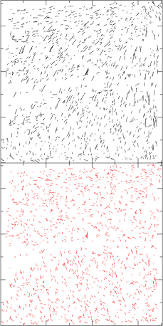
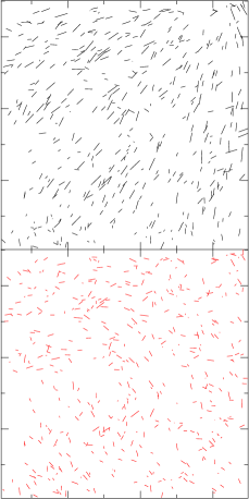
Figure 2.— Ellipticity patterns measured onto stars in all the COSMOS (left) and SLACS (right) fields. Upper (black) panels show stellar ellipticities before applying PSF correction scheme whereas the lower (red) panels show that the main distortion patterns are significantly suppressed after correction. Each panel corresponds to the full ACS field of view (i.e. $200\arcsec$ on a side)

Fig. 2 shows the ellipticity of stars before and after our PSF correction scheme for the 100 COSMOS fields and our 22 SLACS fields. Averaged over the COSMOS fields we measured a mean complex ellipticity $\langle e_{*,{\rm uncor}}\rangle=(-0.0037+0.0072i)\pm 0.0004$ before PSF anisotropy correction and $\langle e_{*,{\rm cor}}\rangle=(0.0000-0.0043i)\pm 0.0003$ after correction. Similarly, in SLACS fields we obtained $\langle e_{*,{\rm uncor}}\rangle=(-0.0025+0.0096i)\pm 0.0006$ and $\langle e_{*,{\rm cor}}\rangle=(0.0011-0.0023i)\pm 0.0005$. In both datasets the scatter of corrected stellar ellipticities about this mean is isotropic and $\sigma_{e_{*,{\rm cor}}}\simeq 0.0087$. We conclude that the correction reduces the mean PSF anisotropy by a factor $2-4$ although some residuals are still present at the $\sim 0.003$ level. We will show in § 4.2.3 that the residual uncertainties are negligible for our purpose.

In addition to anisotropic distortions, the convolution with the PSF also produces isotropic smearing making objects appear rounder. This effect is much smaller on HST images than from the ground but it must be taken into account for small objects with a typical size comparable to that of the PSF. Our initial size cut $r_{h}\geq 0.09\arcsec$ guarantees that such isotropic smearing is kept at a low level and the KSB method can perform an accurate correction (Kaiser et al. 1995; Hoekstra et al. 1998). Our implementation of KSB builds on the proposed improvements suggested by the STEP1 and STEP2 results (Heymans et al. 2006b; Massey et al. 2007). These papers indicate that, in general, KSB methods can achieve $\sim$10% relative shear calibration biases or smaller. Since this is smaller than our statistical errors, it is sufficient to adopt for the present paper a conservative 10% systematic uncertainty in our shear calibration ($m$ STEP parameter). In a future paper we plan to take advantage of the future spaceSTEP simulation set to get a more accurate estimate of the uncertainty on the shear calibration. This will be necessary given the gain in sensitivity expected when the deep SLACS follow-up will be complete. In addition, we demonstrate in the next section that no significant residual additive term ($c$ STEP parameter) is observed in either the SLACS data or the COSMOS control fields.

4.2.2 Charge Transfer Efficiency

Another source of systematic distortion is the degradation of Charge Transfer Efficiency (CTE) on ACS CCDs. Charges are delayed by defects in the readout direction (i.e.  the $y$ axis, charges going from the gap between the CCD chips toward the field boundaries), imprinting a tail of electrons behind each object which modifies its shape, thus producing a spurious negative $e_{1}$ component. Since the strength of CTE-induced distortions depends on the signal-to-noise (snr) of the objects (the fainter the source the stronger the effect), we cannot measure distortions from stars and correct faint galaxies accordingly. This effect must be quantified and corrected with galaxies themselves but one must be able to distinguish between the physical signal and the CTE distortions. To this aim we use the blank COSMOS fields to make sure that our CTE correction scheme will efficiently remove CTE distortions while leaving the actual shear signal unchanged. In practice, we use the empirical recipe proposed by R07 in which an $e_{1,{\rm CTE}}$ component, function of $y$ pixel coordinate, snr, observation time (since CCD degradation increases with time) is subtracted for each object. Here we adapt the expression from Eq. (10) of R07

$$\begin{split}e_{1,{\rm CTE}}=-3.6\times 10^{-4}\left(\frac{1}{2}-\left|\frac{1}{2}-y^{\prime}\right|\right)\,{\rm snr}^{-0.9}\,\times\,\\ \left({\rm MJD}-52333\right)\left(\frac{r_{h}}{0.18\arcsec}\right)^{-0.1}\end{split}$$ (9)

to the imcat definition of snr whereas R07 use SExtractor. Note that the small dependence of $e_{1,{\rm CTE}}$ on size is somewhat degenerate with the way snr is defined and may not be always necessary (like in R07). Note also that snr is calculated by imcat without taking into account noise correlation caused by multidrizzling on oversampled pixels ($0.03\arcsec$ pixel size instead of the native $0.05\arcsec$ value). Therefore this expression may not be directly applicable with different multidrizzle settings. MJD is the Modified Julian Date of observation, $r_{h}$ is the half-light radius and $y^{\prime}$ is the normalized $y$ pixel coordinate.

Fig. 3 illustrates the effect of CTE on $e_{1}$ ellipticity components for COSMOS and SLACS fields (respectively left and right panels). We show the $e_{1}$ component of galaxy ellipticity as a function of the $y^{\prime}$ frame coordinate for sources brighter than I$=27$ (i.e. well beyond our magnitude cut for selecting suitable sources). The upper panels show the mean $e_{1}$ before and after CTE(+PSF) correction. For COSMOS and SLACS we see a similar tendency for vertical stretching of galaxies in the middle of the frame. The empirical CTE distortion fitting formula (9) provides a good correction. Although statistical errors are larger in the SLACS images (5 times smaller sample) we see a modulation of the corrected $e_{1}$ component as a function of $y^{\prime}$ that is not observed in the corrected COSMOS images. As we shall see below this is the signature of the signal we are interested in and it should not be erased by the CTE correction scheme (in order to compare this residual with the expected shear, we overlay the $\langle e_{1}(y^{\prime})\rangle$ shear signal from an isothermal sphere with Einstein Radius $R_{\rm Ein}=1.2\arcsec$). The lower panels (left and right) show how CTE distortions depend on signal to noise ratio. We have split the galaxy sample into three magnitude quantiles, the bright objects being less distorted. This is well accounted for by the snr (and size) dependence in Eq. (9). The overall amplitude of CTE distortion is approximately double for SLACS images because of increasing CCD degradation with time. This is also well captured by Eq. (9). The median observation date of the 100 COSMOS exposures we are considering is $\overline{MJD}_{\rm cosmos}=53141$ and for SLACS it is $\overline{MJD}_{\rm slacs}=53972$.

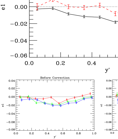
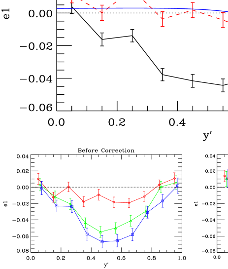
Figure 3.— Vertical spurious stretching (negative $e_{1}$ ellipticity component) as a function of vertical pixel coordinate due to CTE degradation. Measurements for COSMOS and SLACS fields are shown in the left and right panels respectively.     Upper panels: average stretching before (solid black) and after (dashed red) applying our empirical correction term. Distortions are maximum far from the readout (gap between CCDs at $y^{\prime}\sim 0.5$). They are stronger in SLACS images because the number of defects in CCDs increases with time. The corrected residual signal should not perfectly “flat” in SLACS fields because of the presence of the true weak lensing signal we aim at detecting. The amplitude of the mean $e_{1}$ shear signal expected from an isothermal sphere with Einstein Radius $R_{\rm Ein}=1.2\arcsec$ is shown for comparison (solid blue).     The lower left and lower right panels show that distortions are stronger for fainter objects as illustrated by splitting galaxies into three magnitude bins (red, green, blue curves for bright, intermediate and faint objects). Comparing $e_{1}$ ellipticities before (left) and after (right) applying our correction scheme, we see that equation (9) corrects this spurious signal at all magnitudes.

4.2.3 Checks on residuals

To test the quality of the instrumental systematics correction, we plot in Fig. 4 the radial profile of both the tangential $e_{t}$ and curl $e_{\times}$ components of the complex ellipticity in COSMOS and SLACS fields (left and right respectively). The center is set on the lens for SLACS images and at the same location in the detector frame in COSMOS. If we first focus on these latter images, we see no statistically significant residual $e_{t}$ nor $e_{\times}$ component, thus showing that we are free from PSF (seen in stars and galaxies) or CTE (seen in galaxies only) systematics. As well around SLACS lenses, stars do not carry any significant residual $e_{t}$ or $e_{\times}$ signal. Therefore we can safely assume that our systematics correction scheme is accurate enough for the present analysis. Galaxies in SLACS fields clearly carry a strong $e_{t}$ signal (note the first data point well outside the plotting window) whereas no statistically significant $e_{\times}$ component is observed as expected for a gravitational lensing origin of this shear signal.

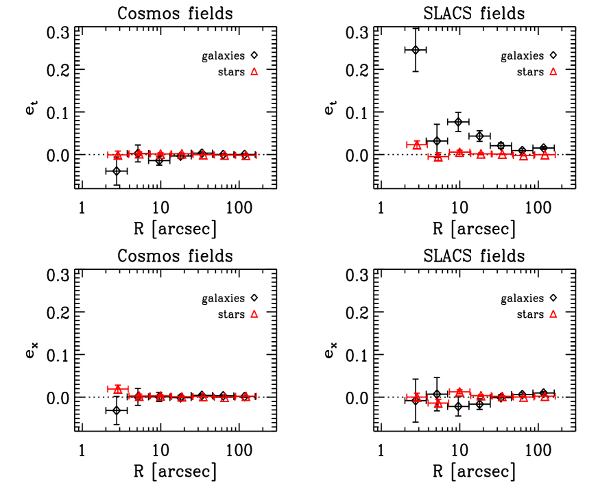
Figure 4.— Radial ellipticity profile in COSMOS left and SLACS right fields. Upper panels show the tangential component $e_{t}$ profile and lower panels show the curl component $e_{\times}$. The signal is measured on both distortion-corrected stars (red triangles) and galaxies (black squares). For plotting convenience the innermost data point in the upper right panel ($e_{t}$ in SLACS) falls outside the window.

4.3. Other sources of error

A final additional potential source of systematic uncertainy is the effect of the lens galaxy surface brightness on the ellipticity of background sources at small projected radii. To estimate this effect, we detected and measured object shapes before and after subtraction of the lens surface brightness profile using galfit and b-spline techniques developed for the strong lensing analysis (paper I). These two method yield similar results for the purpose of weak lensing. It turns out that the lens-subtraction process changes measured ellipticities by at most 5% in an incoherent way. Therefore we do not consider further the effect of lens surface brightness as a relevant potential source of systematic.

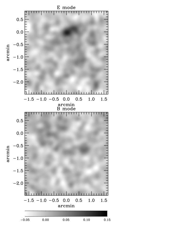
Figure 5.— Mass reconstruction around stacked SLACS lenses in the same detector frame. The upper panel shows the convergence map (E-mode) whereas the lower panel shows the recovered convergence map after rotating galaxies by $45^{\circ}$ (B-mode) which is consistent with a pure noise realization.

4.4. Two-dimensional mass reconstruction and shear profile

In the upper panel of Fig. 5 a mass reconstruction (convergence $\kappa$ map) around the stacked lenses using the Kaiser & Squires (1993) method is shown. There is only one significant convergence peak at the position of the main lens. Note that the Gaussian smoothing scale of the convergence maps is 8 arcsec. This extraordinary high spatial resolution is made possible by the high density of background sources. The lower panel shows the imaginary part of the reconstructed mass map (obtained after rotating background galaxies by $45^{\circ}$). This is consistent with a pure noise map and illustrates the amplitude of the noise.

We now analyze the radial shear profile achieved by stacking the lens galaxies. Since the images are taken at a random orientation with respect to the lens major axis we can safely assume circular symmetry in the analysis. We convert the shear $\gamma$ into the physical quantity $\Delta\Sigma(R)=\Sigma_{\rm crit}\gamma(R)=\overline{\Sigma}(<R)-\Sigma(R)$. For a given lens redshift $z_{\rm l}$ we also define the average critical density $\Sigma_{\rm crit}^{\prime}=\frac{c^{2}}{4\pi G}\frac{1}{D_{\rm ol}\overline{w}(z_{\rm l})}$. An estimator for $\Delta\Sigma$ at a given radius is

$$\Delta\Sigma=\frac{\sum_{j=1}^{N_{\rm lens}}{\Sigma_{\rm crit}^{\prime}}_{j}^{-1}\sum_{i=1}^{N_{s,j}}e_{t,i}\sigma_{e,i}^{-2}}{\sum_{j=1}^{N_{\rm lens}}{\Sigma_{\rm crit}^{\prime}}_{j}^{-2}\sum_{i=1}^{N_{s,j}}\sigma_{e,i}^{-2}}$$ (10)

where $N_{s,j}$ is the number of sources in the radial bin around lens $j$ and $\sigma_{e,i}$ is the uncertainty assigned to the tangential ellipticity estimate $e_{t,i}$ (see Gavazzi & Soucail 2006, for details on this weighting scheme). With this definition, $\Delta\Sigma$ is directly comparable to other SDSS weak galaxy-galaxy lensing analyses (e.g. S04, M06).

Measured $\Delta\Sigma$ values around SLACS lenses are reported in Tab. 2 and shown in Fig 6. The detection significance is derived as follows. The $\chi^{2}$ of the data with respect to the zero shear hypothesis is 47.8 for 9 degrees of freedom. The probability of finding a higher $\chi^{2}$ is $3\times 10^{-7}$, thus the non-detection hypothesis is rejected at the 99.99997% level. For a Gaussian distribution this is equivalent to 5$\sigma$.

To compare with previous studies, we consider the measurement from S04 for their subsample of massive $\sigma_{v}>186\,{\rm km\,s}^{-1}$. The mean square velocity of their sample is $\langle\sigma_{v}^{2}\rangle^{1/2}\simeq 225\,{\rm km\,s}^{-1}$. In order to compare with our points we need to correct for the different velocity dispersion. Assuming an isothermal profile, the shear scales as the velocity dispersion squared, so that we need to scale their points up by $(248/225)^{2}\sim 1.21$ for a proper comparison. After this correction, the agreement is excellent in the radial range $60\lesssim R\lesssim 200\,h^{-1}\,{\rm kpc}$ of overlap as shown in Figure 6. We also check that our results are in agreement with the $\Delta\Sigma$ profile of the sm7 (early-type) stellar mass bin of M06.

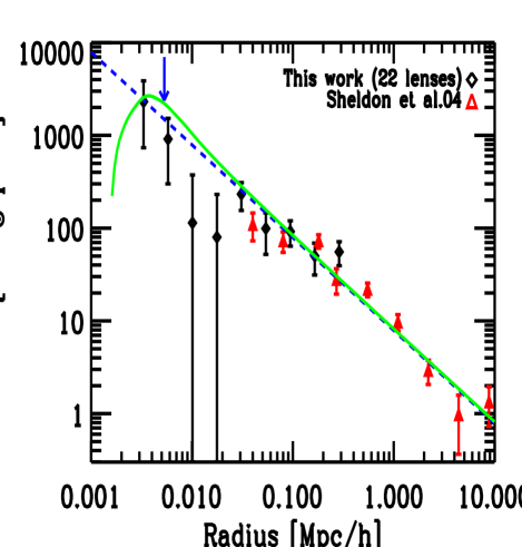
Figure 6.— Radial shear profile around 22 SLACS strong lenses (black diamonds) expressed as the excess surface mass density $\Delta\Sigma(R)$. SLACS bin are completely uncorrelated. The blue arrow denotes the mean effective radius of the lenses stellar component $\overline{R_{\rm eff}}\simeq 5.3\,h^{-1}\,{\rm kpc}$. The average critical density is $\Sigma_{\rm crit}\simeq 4620\,h\,{\rm M}_{\odot}\,\,{\rm pc}^{-2}$. Previous results from S04 scaled to the same average square velocity dispersion are shown for comparison as red triangles (see § 4.4 for details). The curves show the shear profile expected from strong lensing SIS models. This is not a fit. The solid green curve takes into account non linear effects in the relation $\langle e\rangle=g=w\gamma/(1-w\kappa)$ whereas the dashed blue line neglects non linearities. This shows that $\langle e\rangle=\overline{w}\gamma$ is a good approximation for our purposes.

Table 2Measured excess surface density $\Delta\Sigma$ and shear $\gamma$

Proj. Radius	$\Delta\Sigma$	$\Delta\Sigma_{\times}$	$\sigma_{\Delta\Sigma}$	$\gamma_{t}$	$\gamma_{\times}$	$\sigma_{\gamma}$
$\,h^{-1}\,{\rm kpc}$	$\,h{\rm M}_{\odot}/\,{\rm pc}^{2}$	$\,h{\rm M}_{\odot}/\,{\rm pc}^{2}$	$\,h{\rm M}_{\odot}/\,{\rm pc}^{2}$
3.3	2307	-1015	1570	0.339	-0.054	0.093
5.8	918	-526	614	0.206	-0.095	0.078
10.1	115	141	264	0.074	0.010	0.047
17.6	81	-180	153	0.028	-0.011	0.029
30.8	232	-36	80	0.064	-0.005	0.017
53.9	100	36	46	0.019	0.001	0.010
94.1	90	-45	27	0.016	-0.010	0.006
164.5	52	52	17	0.010	0.014	0.005
287.5	60	34	17	0.014	0.008	0.004

The curl component $\Delta\Sigma_{\times}=\Sigma_{\rm crit}\gamma_{\times}$ is statistically consistent with zero. $\sigma_{\Delta\Sigma}$ is $1\sigma$ error on both $\Delta\Sigma$ and $\Delta\Sigma_{\times}$. $\sigma_{\gamma}$ is $1\sigma$ error on both $\gamma_{t}$ and $\gamma_{\times}$.

5. Joint Strong & Weak lensing modeling

In this section we take advantage of the availability of both strong and weak lensing constraints to investigate the mass profile of SLACS lenses from a fraction of the effective radius to 100 effective radii ($3\lesssim R\lesssim 300\,h^{-1}\,{\rm kpc}$).

5.1. SIS consistency check

Before considering more sophisticated models for the density profile, we first check if the singular isothermal density profile favored in the inner parts of galaxies by strong lensing alone (e.g.  Rusin et al. 2003), and by strong lensing and stellar dynamics (Treu & Koopmans 2004, paper III), is consistent with our weak lensing measurements.

5.1.1 Consistency with strong lensing

For a singular isothermal sphere (SIS) the convergence profile as a function of radius $R$ is:

$$\kappa(R)=\frac{R_{\rm Ein}}{2R}=\gamma(R)\>,$$ (11)

with $R_{\rm Ein}=4\pi(\sigma_{\rm SIS}/c)^{2}D_{\rm ls}/D_{\rm os}$ in radians and $\sigma_{\rm SIS}$ the lensing-inferred velocity dispersion which turns out to be very close to the stellar velocity dispersion $\sigma_{*}$ of the lens galaxy (paper II). For a proper comparison, weak and strong lensing measurements have to be renormalized to the same source plane. Hence the Einstein radius given by strong lens modeling has to be rescaled by a factor $\overline{w}_{\rm WL}/w_{\rm SL}$ (see Table 1). Fig. 6 shows that after this scaling, but without fitting any free parameter, the strong lensing SIS models provide a reasonably good description of SLACS weak lensing data out to $\sim 100\,h^{-1}\,{\rm kpc}$ (with $\chi^{2}/{\rm dof}\simeq 22.8/9\simeq 2.5$), and of the SDSS data beyond that (with $\chi^{2}/{\rm dof}\simeq 27.6/9\simeq 2.7$). Two models are shown: one that neglects the non-linear relation between reduced shear and ellipticity (blue dashed) and one that takes this effect into account as well as the associated non-linear dependence on the source redshift distribution (solid green). The two curves differ by less than the error bars of our measurements, showing that a linear relation between ellipticity and shear is a reasonable approximation given the present statistical errors. This analysis shows that the total mass density profile of the SLACS lenses is very close to an isothermal sphere with velocity dispersion equal to the stellar velocity dispersion. Since the luminous component is steeper than isothermal outside the effective radius, this finding implies the presence of an extended dark matter halo which is in turn shallower than isothermal at similar radii.

5.1.2 Consistency with strong lensing and stellar dynamics

A simple – although model dependent – way to compare on the same plot the mass measurement obtained with strong lensing, stellar dynamics and weak lensing is obtained in the following manner. For each radial bin we can define an effective weak lensing velocity dispersion as the velocity dispersion of the singular isothermal sphere that reproduces the shear in that bin. The effective weak lensing velocity dispersion profile is shown in Figure7 together with the average stellar velocity dispersion determined from SDSS spectroscopy and the average stellar velocity dispersion of the singular isothermal ellipsoid that best fits the strong lensing configuration.

The figure illustrates the complementarity of the three mass tracers, stellar velocity dispersion well inside the Einstein Radius, strong lensing at the Einstein radius, and weak lensing outside the Einstein radius, as well as the dynamic range of the measurement, almost three decades in radius. The very close correspondence of the stellar and strong lensing measurement was discussed in paper II, and is confirmed here for a larger sample of lenses. This paper shows that, albeit with larger uncertainties, the weak lensing data show that the profile is approximately flat for another two decades in radius. This is a qualitative statement as a full joint (strong+weak) lensing and dynamical analysis is needed to combine the three diagnostics properly. The three-pronged analysis is beyond the scope of this paper and is left for future work. In the rest of this paper we will focus on combining strong and weak lensing in the context of a two-component mass model.

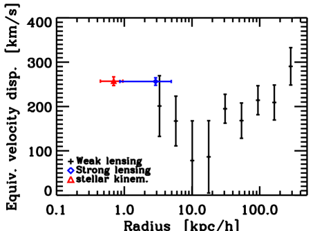
Figure 7.— Illustration of the complementarity of three mass tracers (stellar velocity dispersion, effective strong and weak lensing velocity dispersion) over almost three decades in radius. Stellar velocity dispersion constrains the innermost regions ($\ll R_{\rm Ein}$), strong lensing the region around the Einstein radius, while weak lensing is most effective beyond the Einstein radius.

5.2. Two component models

In the rest of this section we perform a joint strong and weak lensing analysis of the data, in order to disentangle the mass profile of the stellar component and of the surrounding dark matter halo. For this purpose we adopt a simple two component model as detailed below. For simplicity, we assume that all lenses are at the center of their halo and none of them is an off-center satellite in a bigger halo. This approximation is well motivated by the galaxy-galaxy lensing results of M06 who found that only a small fraction ($\lesssim 15\%$) of massive ellipticals do not reside at the center of their host halo. Strictly speaking, the quantity measured by weak lensing is the projected galaxy-mass cross-correlation function rather than the actual shear profile of an individual halo. However, the interpretation of this cross-correlation function within the successful framework of the “halo model” (e.g.  Cooray 2006) allows one to disentangle the contribution of the proper halo attached to a given galaxy (1-halo central term), the halo of a more massive host galaxy (or group or cluster) if this galaxy is a satellite (1-halo satellite term), and the contribution due to clustering of neighboring halos about the main halo attached to the galaxy (2-halo term). However, the 2-halo terms only provide a significant contribution to the galaxy-mass cross-correlation function beyond a few Mpc (as compared to the outermost $\sim 300\,h^{-1}\,{\rm kpc}$ radial bin probed here) and our lenses are massive ellipticals and thus most likely central galaxies. Therefore for the purpose of this analysis, and given the measured uncertainties, we can assume with little loss of accuracy that the measured shear profile is representative of the only surrounding main halo (see e.g. Fig. 1 of Mandelbaum et al. 2005).

5.2.1 Model definition

We model the stellar component with a de Vaucouleurs density profile (de Vaucouleurs 1948; Maoz & Rix 1993; Keeton 2001) The effective radius of the stellar component is fixed to the ACS surface photometry. Thus the only free parameter needed to measure the luminous component is the average stellar mass-to-light ratio $\Upsilon_{V}$. The dark matter halo is assumed to be of the NFW form (Navarro et al. 1997; Bartelmann 1996; Wright & Brainerd 2000) in which the density reads

$$\rho(r)=\rho_{c}\delta_{c}\left(\frac{r}{r_{s}}\right)^{-1}\left(1+\frac{r}{r_{s}}\right)^{-2}\,.$$ (12)

with $r_{s}$ the scale radius and $\rho_{c}$ the Universe critical density. The term $\delta_{c}=\frac{\Delta}{3}c^{3}/\left[\ln(1+c)-c/(1+c)\right]$ relates the so-called concentration parameter $c=r_{\Delta}/r_{s}$. We assume an overdensity of $\Delta=119$ so that $r_{\Delta}$ can be considered the “virial” radius (Bryan & Norman 1998). This definition agrees with those of Hoekstra et al. (2005) and Heymans et al. (2006a) for our assumed $\Lambda$CDM cosmology. Because statistical errors are still large with only 22 SLACS lenses used here, we lack the sensitivity to constrain the dark matter profile in detail. Thus, instead of fitting a free concentration parameter, we assume the general relation observed in numerical simulations:

$$c=\frac{9}{1+z}\left(\frac{M_{\rm vir}}{8.12\times 10^{12}\,h^{-1}{\rm M}_{\odot}}\right)^{-0.14}\,,$$ (13)

(Bullock et al. 2001; Eke et al. 2001; Hoekstra et al. 2005). In addition, we are not able to constrain the virial mass of each lens individually, so we need to assume a scaling relation between virial mass and V band luminosity of the form: $M_{\rm vir}=\tau_{V}L_{V}$. Note that we check that assuming a steeper relation $M_{\rm vir}\propto L_{V}^{1.5}$ (Guzik & Seljak 2002; Hoekstra et al. 2005; Mandelbaum et al. 2006) yields comparable results because the SLACS lenses span a narrow range in luminosities, with 0.2 dex rms around $\langle L_{V}\rangle=5.70\times 10^{10}\,h^{-2}\,{\rm L}_{\odot}$. In conclusion, our model has only two free parameters, the mass-to-light ratio of the luminous component $\Upsilon_{V}$ and the virial mass-to-light rato $\tau_{V}$.

Having defined the model, we now define the merit function that will be used to determine the best fitting parameters with their uncertainties. Detailed strong lensing analysis of multiply imaged sources have shown that extremely tight constraints can be set on the Einstein radius of individual lenses (e.g. paper III), with typically a few percents relative accuracy $\sigma_{R_{\rm Ein}}/R_{\rm Ein}\simeq 5\%$. This can be interpreted as a surface mass measurement since the mean density $\overline{\Sigma}$ within this radius is by definition equal to the critical density $\Sigma_{\rm crit}$. Therefore for each lens we are able to write:

$$\overline{\Sigma}(<R_{\rm Ein})=\Sigma_{\rm crit}(z_{\rm l},z_{\rm s})\;.$$ (14)

The relative error on $R_{\rm Ein}$ translates into $\sigma_{\overline{\Sigma}}/\overline{\Sigma}\simeq 5\%$. We can thus define a strong lensing merit function:

$$\chi^{2}_{\rm sl}=\sum_{i=1}^{N_{\rm lens}}\left(\frac{{\Sigma_{\rm crit}}_{,i}-\overline{\Sigma}_{*,i}(\Upsilon_{V})-\overline{\Sigma}_{DM,i}(\tau_{V})}{\sigma_{\overline{\Sigma}}}\right)^{2}$$ (15)

where subscripts $*$ and $DM$ stand for luminous and dark matter components, evaluated at position ${R_{\rm Ein}}_{i}$.

In a complete analogy, we define the weak lensing merit function:

$$\begin{split}\chi^{2}_{\rm wl}&=\sum_{j=1}^{N_{\rm rbin}}\frac{1}{\sigma_{\Delta\Sigma,j}^{2}}\\ &\left[\Delta\Sigma_{j}-\frac{1}{N_{\rm lens}}\sum_{i=1}^{N_{\rm lens}}\left(\Delta\Sigma_{*,ij}(\Upsilon_{V})+\Delta\Sigma_{DM,ij}(\tau_{V})\right)\right]^{2}\end{split}$$ (16)

where $N_{\rm rbin}$ is the number of radial bins $r_{j}$ at which $\Delta\Sigma_{j}=\Delta\Sigma(r_{j})$ is obtained from the weak lensing data shown in Fig. 6.

In the next section we will derive the best fitting $\{\Upsilon_{V},\tau_{V}\}$ values that minimize the total $\chi^{2}=\chi^{2}_{\rm sl}+\chi^{2}_{\rm wl}$.

5.2.2 Results

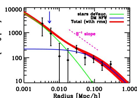
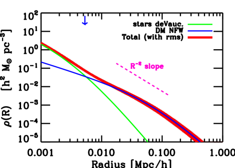
Figure 8.— Upper panel: Shear profile (i.e. $\Delta\Sigma$) for the best DM + de Vaucouleurs profile. The contribution of each mass component is detailed (green and blue for stars and DM respectively). The thickness of the red curve codes for the $1\sigma$ uncertainty around the total shear profile. Uncertainties are very small below 10 kpc because of strong lensing data that cannot be shown here. Lower panel: Similar coding for the three-dimensional density profile $\rho(R)$. The transition between star- and DM-dominated mass profile occurs close to the mean effective radius (blue arrow). The total density profile is close to isothermal over $\sim 2$ decades in radius.

The upper panel of Fig. 8 shows the radial profile of the shear for the best fit model together with weak lensing data points. The fit is excellent with a $\chi^{2}/{\rm dof}=29.1/31\simeq 0.94$. We see the detail of the contribution of stellar and dark matter components. This joint strong+weak lensing analysis allows to disentangle the contribution of each. Because the latter component is less concentrated and more extended than the former, there is a radial range $R\sim 20\,h^{-1}\,{\rm kpc}$ at which surface mass density flattens. This implies a fast drop in the shear profile $\Delta\Sigma(R)$ at that scale which is quite easy to detect.

In the lower panel of Fig. 8 we show the corresponding three-dimensional mass density profile $\rho(R)$. This profile is close to isothermal although it is made of two components which are not isothermal. The components combine to make an almost isothermal density profile at scales $R\lesssim 100\,h^{-1}\,{\rm kpc}$ with a transition from star-dominated to dark matter dominated profiles occurring close to the effective radius.

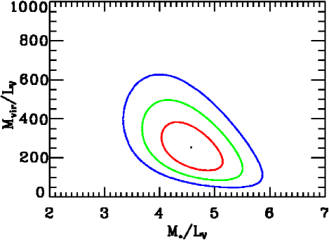
Figure 9.— Confidence levels around model parameters (1, 2 and 3 $\sigma$ contours) for the relation between total virial mass-to-light ratio $\tau_{V}=M_{\rm vir}/L_{V}$ and stellar mass-to-light $\Upsilon_{V}=M_{*}/L_{V}$ ratio. Given the sample mean luminosity $\langle L_{V}\rangle=5.7\times 10^{10}\,h^{-2}L_{\odot}$, we find a mean sample stellar mass $\langle M_{*}\rangle=2.55\pm 0.27\times 10^{11}\,h^{-1}{\rm M}_{\odot}$ and virial mass $\langle M_{\rm vir}\rangle=14^{+6}_{-5}\times 10^{12}\,h^{-1}{\rm M}_{\odot}$.

The best fit NFW + de Vaucouleurs lens model yields a stellar mass-to-light ratio $\Upsilon_{V}=4.48\pm 0.46\,h{\rm M}_{\odot}/L_{\odot}$ and virial mass-to-light ratio $\tau_{V}=246^{+101}_{-87}\,h{\rm M}_{\odot}/L_{\odot}$. This translates into a virial to stellar mass ratio $M_{\rm vir}/M_{*}=54^{+28}_{-21}$. Note that stellar mass-to-light ratio depends in the same way on $h$ as virial mass as they are inferred from lens modeling and not from stellar evolution models. Thus $M_{\rm vir}/M_{*}$ is independent of $h$. Fig. 9 shows the 68.3, 95.4 and 99.7% confidence levels contours for the best fit model parameters. A model having a constant mass-to-light ratio (i.e. $M_{\rm vir}/L_{V}=0$) is ruled out at $\sim 4\sigma$.

Given the sample mean luminosity $\langle L_{V}\rangle=5.7\times 10^{10}\,h^{-2}L_{\odot}$, we find a mean sample stellar mass $\langle M_{*}\rangle=2.55\pm 0.26\times 10^{11}\,h^{-1}{\rm M}_{\odot}$ and virial mass $\langle M_{\rm vir}\rangle=14^{+6}_{-5}\times 10^{12}\,h^{-1}{\rm M}_{\odot}$. This translates into a mean virial (resp. scale) radius $r_{\rm vir}=393^{+47}_{-53}\,h^{-1}\,{\rm kpc}$ (resp. $r_{s}=58\pm 8\,h^{-1}\,{\rm kpc}$). We note that the virial radius is typically larger that our field of view, and therefore virial masses rely on extrapolations of our results. Therefore, we also present more robust measurements like the projected and three-dimensional mass within a reference radius $R=200\,h^{-1}\,{\rm kpc}$. Lens modeling yields $M_{3D}(<200\,h^{-1}\,{\rm kpc})=(8.1\pm 1.8)\times 10^{12}\,h^{-1}{\rm M}_{\odot}$ and a projected mass $M_{2D}(<200\,h^{-1}\,{\rm kpc})=(10.8\pm 2.7)\times 10^{12}\,h^{-1}{\rm M}_{\odot}$ (68% CL errors).

To compare with local measurements we convert our $\Upsilon_{V}$ mass-to-light ratio to the rest-frame B band. Assuming a typical $(B-V)=0.96$ color for Ellipticals (Fukugita et al. 1995), $(B-V)_{\odot}=0.65$ and a Hubble constant $h=0.7$, one finds $\Upsilon_{B}=4.17\pm 0.44\,{\rm M}_{\odot}/{\rm L}_{\odot}$. Using paper II, Treu & Koopmans (2004) and similar findings (Treu & Koopmans 2002; Treu et al. 2005; van der Wel et al. 2005; di Serego Alighieri et al. 2005) for the passive evolution of massive early-type galaxies, we get a redshift zero B band stellar mass-to-light ratio $\sim 5.81\pm 0.61$ which is statistically consistent with local estimates such as $\Upsilon_{B}=7.8\pm 2.7$ and $\Upsilon_{B}=7.1\pm 2.8$ from Gerhard et al. (2001) and Trujillo et al. (2004) respectively. The low value of $M_{*}/L$ is also in broad agreement with stellar evolution models of Bruzual & Charlot (2003), although detailed comparisons depend on the assumed Initial Mass Function (IMF).

Our modeling can be used relate the V band luminosity within the Einstein radius $\overline{L}_{V}(<R_{\rm Ein})$ and the fraction of dark matter in the same projected radius $f_{DM,2d}(<R_{\rm Ein})$. Using Eq. (14), for a given stellar mass-to-light ratio each lens must verify

$$f_{\rm DM,2d}(<R_{\rm Ein})=1-\Upsilon_{V}\overline{L}_{V}{(<R_{\rm Ein})}/\Sigma_{\rm crit}\,.$$ (17)

Fig. 10 shows the inferred projected $f_{\rm DM,2d}$ using our best fit $\Upsilon_{V}=4.48\,h^{-1}{\rm M}_{\odot}/{\rm L}_{\odot}$. The mean dark matter fraction within the Einstein radius $\langle f_{\rm dm,2d}\rangle=0.37\pm 0.04$ with $18\%$ rms scatter. Extrapolating to the effective radius, about half of the projected mass is in the form of dark matter. The result from the NFW + de Vaucouleurs parameterization is shown as the solid curve which matches the data points well (see also papers II and III). This parameterization also allows the deprojected dark matter fraction to be calculated, and is found to be $\sim 27\%$ (dotted blue line) within $R_{\rm eff}$. The local deprojected DM and stellar densities are of the same order at that radius.

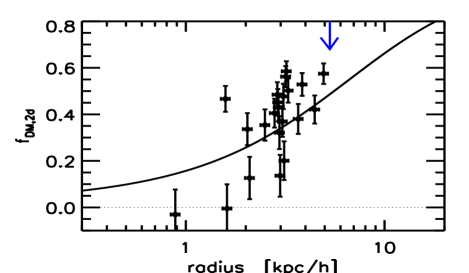
Figure 10.— Projected dark matter fraction in SLACS lenses as measured from strong lensing at the Einstein radius (data points) and our constraints on the stellar $M_{*}/L$ ratio. The Einstein radius is expressed in physical units and the solid curve shows the best fit profile of the dark matter fraction $f_{\rm DM,2d}$ inferred from the parametric NFW + de Vaucouleurs modeling of strong+weak lensing data. The mean effective radius is shown as a blue arrow. We see that $f_{\rm DM,2d}(<R_{\rm eff})\simeq 50\%$ of the projected enclosed mass is in the form of dark matter within the effective radius.

It may seem that the two data points with $f_{\rm dm,2d}\simeq 0$ are responsible for our inferred low $M_{*}/L$. Since these two lenses have the most elongated stellar component, the assumption of circular symmetry may break down for them. Furthermore, if they have a disk component with younger starsq, this could reduce their global $M_{*}/L$ with respect to that of pure spheroidal systems. However, redoing the strong+weak lens modeling without these does not change the stellar mass-to-light ratio to significantly ($M_{*}/L_{V}=4.90\pm 0.53\,h^{-1}{\rm M}_{\odot}/{\rm L}_{\odot}$).

5.3. Comparison to previous galaxy-galaxy lensing works

We first compare our findings to the SDSS weak galaxy-galaxy lensing analysis of M06 who defined $M_{\rm cent}$ as the mass enclosed in a sphere within which the mean density is 180 times the background density, similar to our definition. Our lens sample should be compared to the sm7 stellar mass bin for early-type galaxies with $\langle M_{*}\rangle=39.6\times 10^{10}{\rm M}_{\odot}$. It would also lie between l6b and l6f early-type galaxy luminosity bins with a typical $\langle L\rangle\simeq 6.3L_{*}$. To convert the rest frame V band to the SDSS $r^{\prime}$ band we use $V-r^{\prime}\simeq 0.36$ for Ellipticals (Fukugita et al. 1995). Since at the exponential tail of the luminosity and mass functions one is highly sensitive to the scatter in the mass-luminosity relation, M06 applied corrections calibrated into simulations (Mandelbaum et al. 2005) whereas our analysis does not attempt to correct for this effect. For the l6f bin, $M_{\rm cent}/L_{r}=674^{+210}_{-203}\,h{\rm M}_{\odot}/{\rm L}_{\odot}$ as found by M06 yields $M_{\rm cent}/L_{V}=896\pm{275}\,h{\rm M}_{\odot}/{\rm L}_{\odot}$ (95% CL). Likewise the sm7 bin of M06 yields $M_{\rm cent}/M_{*}=256^{+44}_{-68}$ (95% CL and using $h=0.7$). These values are significantly larger than our results. However if we apply a similar correction as these authors our virial mass should be raised by 66%, yielding $M_{\rm vir}/L_{V}=408^{+168}_{-144}\,h{\rm M}_{\odot}/{\rm L}_{\odot}$ and $M_{\rm vir}/M_{*}=89^{+46}_{-35}$. This latter correction thus brings our findings into statistical agreement. The small difference might be due to our inability to probe the very outer parts of halos and efficiently constrain virial masses. However, we emphasize that the availability of strong lensing constraints put tight constraints on the column density enclosed by $R_{\rm Ein}$, which means that the outer parts of halos cannot contribute much in making lens galaxies critical, or perhaps to the fact that we fit for $M_{*}/L$, while M06 use the value determined from stellar population synthesis models. Issues related to comparisons between Guzik & Seljak (2002) and M06 results are addressed in the latter paper. In any case, we find a much better agreement between our $M_{\rm vir}$ measurement and those of Guzik & Seljak (2002) which give $M_{\rm vir}/L_{V}\simeq 296\pm 51\,h{\rm M}_{\odot}/{\rm L}_{\odot}$ after matching our lens sample selection.

We now compare our analysis with the Hoekstra et al. (2005) results. Since we chose to match their definition of virial mass and concentration, we expect comparisons to be easier although the mean redshift of their lens sample is $\sim 0.32$. Our lens sample would passively brighten to $\langle L_{V}\rangle\simeq 6.3\times 10^{10}\,h^{-2}\,{\rm L}_{\odot}$ at $z=0.32$ which is $\sim 2.45$ times brighter than their higher luminosity bin having $L_{V}\simeq 2.45\times 10^{10}\,h^{-2}\,{\rm L}_{\odot}$. Therefore we need to extrapolate their results using their $M_{\rm vir}\propto L^{1.5}$ relation. They find $M_{\rm vir}/L_{V}\simeq 253^{+38}_{-35}\,h{\rm M}_{\odot}/{\rm L}_{\odot}$. This value is statistically consistent with ours. However, a detailed comparison is made difficult due to the fact that the authors mix early- and late-type galaxies and they avoid lens galaxies in dense environments. Using stellar evolution models, they estimate the virial to stellar mass in their reddest subsample $(B-V)_{\rm rest}\sim 0.95$ to be $M_{\rm vir}/M_{*}\simeq 43\pm 6$ for a scaled Salpeter IMF (Bell & de Jong 2001) or $M_{\rm vir}/M_{*}\simeq 27\pm 4$ for a PEGASE Salpeter IMF. The Scaled Salpeter IMF hypothesis turns out to be in better agreement with our measurements. In addition it predicts stellar mass-to-light ratios $\Upsilon_{B}\sim 4.5$ (Solar units) closer to our estimates than the PEGASE IMF which predicts $\Upsilon_{B}\sim 6.5$.

Finally, Heymans et al. (2006a) measure virial masses of lens galaxies in the range $0.2\leq z_{\rm l}\leq 0.8$ in a narrow range of luminosity $L_{r}=2.4\times 10^{10}\,h^{-2}\,{\rm L}_{\odot}$ with a 0.2 dex dispersion about this mean. This sample is dominated by early-type galaxies. Again, extrapolation to our sample mean luminosity is somewhat uncertain but, using the $M_{\rm vir}\propto L_{V}^{1.5}$ scaling, their results give $M_{\rm vir}/M_{*}=76\pm 25$ which is in excellent agreement with our $M_{\rm vir}/M_{*}=54^{+28}_{-21}$.

These comparisons show that our virial mass estimates are in good agreement with other studies after extrapolation of our constraints on the radial shear profile (ending around $\sim 300\,h^{-1}\,{\rm kpc}$) out to the virial radius $\sim 480\,h^{-1}\,{\rm kpc}$. Comparing with other results obtained for less massive systems on average increases uncertainties. However our results on the halo virial masses are well consistent with this ensemble of results above as they lie in between them. In addition, the measured shear profile remarkably match those of S04 and M06 in the radial range $30\lesssim R\lesssim 300\,h^{-1}\,{\rm kpc}$. This gives a valuable support to the validity of our results and the control of systematic effects.

6. Discussion

Our joint weak+strong lensing modeling of SLACS lenses with a two-component mass model allowed us to successfully disentangle the contribution of each giving sensible results for both the stellar mass-to-light ratio $M_{*}/L_{V}=4.48\pm 0.46\,h{\rm M}_{\odot}/{\rm L}_{\odot}$ and virial mass-to-light ratio $M_{\rm vir}/L_{V}=246^{+101}_{-87}\,h{\rm M}_{\odot}/{\rm L}_{\odot}$, in good agreement with other studies. Assuming a NFW and de Vaucouleurs forms for each density profiles provides a good description of the data ($\chi^{2}\simeq 0.94$ per degree of freedom).

This analysis shows that the total density profile is close to isothermal out to $\sim 100\,h^{-1}\,{\rm kpc}$. It is now a well established from SLACS (paper III) and earlier strong lensing studies (e.g.  Treu & Koopmans 2002; Rusin et al. 2003; Rusin & Kochanek 2005; Treu & Koopmans 2004) that the total mass profile of lens galaxies is close to isothermal ($\rho\propto r^{-2}$) within $R_{\rm eff}$. In paper III this result was established by combining strong lensing and stellar kinematics. The present analysis extends and strengthens this results as we find that the dark matter and stellar components combine themselves to form an isothermal total density profile well beyond the effective radius.

We find that the transition from a star-dominated to a dark-matter-dominated density profile must occur close to $R_{\rm eff}$. This peculiar transition is also observed by Treu & Koopmans (2004) which combined strong lensing and stellar kinematics in higher redshift lenses. Similar results can be found in Mamon & Łokas (2005a, b). In addition, the “mean” fraction of DM $f_{dm,3D}(<R_{\rm eff})\sim 30\%$ is in excellent agreement with local estimates (Kronawitter et al. 2000; Gerhard et al. 2001; Borriello et al. 2003), and more recently from the SAURON project (Cappellari et al. 2006). At this point, it is noteworthy to note an important result of paper II, that is, strong lensing galaxies have similar internal properties as normal early-type galaxies in terms of their location in the Fundamental Plane. Our findings can thus be generalized.

We emphasize that we did not investigate other parameterizations for the DM halo. For instance, a steeper profile ($\rho_{DM}\propto r^{-\alpha}$ with $\alpha>1$) could possibly arise from the adiabatic contraction (Blumenthal et al. 1986; Gnedin et al. 2004) of a NFW halo which is found in pure dark matter N-body cosmological simulations made without taking into account the complex physics of baryons. With the small sample of lenses we are considering here, we are not sensitive yet to that level of detail in the inner slope of the assumed DM profiles. We note however that the rather low values of $M_{*}/L_{V}$ we find would make it unlikely to have a dark matter halo much steeper than NFW ($\rho\propto r^{-1}$ at the center) (see also Borriello et al. 2003; Humphrey et al. 2006). Since it is reasonable to assume that baryons somehow perturb the DM halo within the effective radius, we emphasize that our successful NFW parameterization should rather be considered as a fitting formula for the perturbed halo. In future papers, with the complete observed lens sample and spatially resolved measurements of stellar kinematics, we plan to determine with unprecedented accuracy the inner slope of the DM profile below $R_{\rm eff}$ and at the same time $M_{*}/L_{V}$.

The inner regions of lens galaxies can be considered as representative of the whole parent sample of early-type galaxies as shown in paper II. Although there is no firm observational evidence, it is thought that environmental effects may bias the population of lens galaxies since extra convergence coming from surrounding large scale structure may boost lens efficiency while leaving the internal dynamics of lens galaxies unchanged (see also Keeton & Zabludoff 2004; Fassnacht et al. 2006). In the present analysis we address the issue of whether lenses are representative of the overall population at larger radii, by comparing our weak lensing results with those obtained for non-lens samples. The present analysis shows that, on intermediate scales $R_{\rm eff}<R\lesssim 300\,h^{-1}\,{\rm kpc}$, SLACS massive lenses have the same shear properties as normal Ellipticals as found by M06 or S04. We find a good agreement between our virial mass estimates and semi-analytic predictions like those developed in the “halo model” (Mandelbaum et al. 2005, 2006; Cooray 2006). Any systematic environmental effect able to perturb shear measurement on those scale is below our present observational uncertainties. When the ACS follow-up is finished, the weak lensing analysis will provide important new information on the environment of strong lens galaxies. This issue is deferred for a future work.

In terms of the internal structure of early-type galaxies, the present analysis strengthens and extends the results presented in paper III and gives additional support to the picture proposed there for their formation. The isothermal density profile must be produced at early stages of their evolution process ($z\gtrsim 2$) by merging/accretion involving dissipative gas physics to quickly increase the central phase space density since pure collisionless systems would rather develop shallower density slopes $\rho\propto r^{[-1,-1.5]}$ (e.g.  Navarro et al. 1997; Moore et al. 1998; Ghigna et al. 1998; Jing 2000; Navarro et al. 2004). Once isothermality is set, early-type galaxies may evolve passively, or may keep growing quiescently via collisionless “dry” mergers or by accretion of satellites, which preserve the inner density profile of collisionless materials (stars and/or DM). See discussion in paper III and references therein for further details.

7. Summary & Conclusion

We demonstrate that, using deep ACS images, it is possible to measure a weak lensing signal for a modest sample of massive early-type galaxies ($\sigma_{v}\sim 250\,{\rm km\,s}^{-1}$ or $\log M_{*}/{\rm M}_{\odot}\sim 11.35$): with only 22 lenses we are able to detect shear signal at 5$\sigma$ significance. Key to this success is the large density of well-resolved background sources afforded by ACS, which beats down shot noise and reduces the problem of dilution by lens satellites since background sources greatly outnumber satellites. In addition, these lenses are very distant from one another and hence completely statistically independent. Furthermore, special care has been taken to control systematic errors, using the most advanced techniques to model and correct for the ACS PSF and other instrumental effects. By analyzing a sample of 100 blank fields from the COSMOS survey, we show that residual systematics in the shear measurement are less than 0.3%.

Although weak lensing alone can provide interesting results on lens density profiles at intermediate scale, the great power and originality of this work is the combination of strong and weak lensing constraints. Modeling weak and strong lensing in massive ($\langle\sigma_{v}^{2}\rangle^{1/2}\simeq 248\,{\rm km\,s}^{-1}$) SLACS galaxies as a sum of a stellar (de Vaucouleurs) plus dark matter halo (NFW) components, we could disentangle to contribution of the two components overall mass budget. The main results of this joint analysis can be summarized as follows:

• The total density profile is close to isothermal from $0.5R_{\rm eff}\lesssim R\lesssim 100R_{\rm eff}$ although neither the stellar nor the dark matter density profile is isothermal.

• The transition from star- to dark matter-dominated density occurs at $\sim R_{\rm eff}$, leading to a dark matter fraction within this radius $f_{dm,3D}(<R_{\rm eff})=27\pm 4\%$.

• The best fit stellar mass-to-light ratio is $M_{*}/L_{V}=4.48\pm 0.46\,h{\rm M}_{\odot}/{\rm L}_{\odot}$ in agreement with local results and old stellar populations.

• The best fit virial mass-to-light ratio is $M_{\rm vir}/L_{V}=246^{+101}_{-87}\,h{\rm M}_{\odot}/{\rm L}_{\odot}$ in agreement with galaxy-galaxy weak lensing results of non-lens galaxies. We found a mean virial mass and radius $\langle M_{\rm vir}\rangle=14^{+6}_{-5}\times 10^{12}\,h^{-1}{\rm M}_{\odot}$ and $r_{\rm vir}=393\pm 50\,h^{-1}\,{\rm kpc}$ respectively.

• The agreement with other weak lensing studies shows that the outer halos of lenses and non-lenses are consistent within the errors. In other words, if lens early-type galaxies live in peculiar environments, their effect on the shear profile down to $300\,h^{-1}\,{\rm kpc}$ from the lens center are below our statistical errors.

We forecast a $\sim 10\sigma$ detection by the end of the ongoing deep follow-up imaging with HST/ACS. When completed, the SLACS sample of lenses with well resolved kinematics will provide valuable constraints on stellar populations and density profiles of both stellar and dark matter components down to several hundred kiloparsecs of the lens center, thus allowing to address internal properties of lens galaxies as well as the effect of their environment. To complete the picture on early-type galaxiess and structure formation, it is important to extend SLACS results to higher redshift by increasing the number of such strong lenses through new observational efforts.

References

- Arnaboldi et al. (2004) Arnaboldi, M., Gerhard, O., Aguerri, J. A. L., et al. 2004, ApJ, 614, L33
- Bartelmann (1996) Bartelmann, M. 1996, A&A, 313, 697
- Bartelmann & Schneider (2001) Bartelmann, M. & Schneider, P. 2001, Phys. Rep., 340, 291
- Bell & de Jong (2001) Bell, E. F. & de Jong, R. S. 2001, ApJ, 550, 212
- Bertin & Arnouts (1996) Bertin, E. & Arnouts, S. 1996, A&AS, 117, 393
- Bertin et al. (1994) Bertin, G., Bertola, F., Buson, L. M., et al. 1994, A&A, 292, 381
- Blumenthal et al. (1986) Blumenthal, G. R., Faber, S. M., Flores, R., & Primack, J. R. 1986, ApJ, 301, 27
- Bolton et al. (2006) Bolton, A. S., Burles, S., Koopmans, L. V. E., Treu, T., & Moustakas, L. A. 2006, ApJ, 638, 703
- Bolton et al. (2004) Bolton, A. S., Burles, S., Schlegel, D. J., Eisenstein, D. J., & Brinkmann, J. 2004, AJ, 127, 1860
- Borriello et al. (2003) Borriello, A., Salucci, P., & Danese, L. 2003, MNRAS, 341, 1109
- Bradač et al. (2005a) Bradač, M., Erben, T., Schneider, P., et al. 2005a, A&A, 437, 49
- Bradač et al. (2005b) Bradač, M., Schneider, P., Lombardi, M., & Erben, T. 2005b, A&A, 437, 39
- Brainerd et al. (1996) Brainerd, T. G., Blandford, R. D., & Smail, I. 1996, ApJ, 466, 623
- Broadhurst et al. (2005) Broadhurst, T., Takada, M., Umetsu, K., et al. 2005, ApJ, 619, L143
- Bruzual & Charlot (2003) Bruzual, G. & Charlot, S. 2003, MNRAS, 344, 1000
- Bryan & Norman (1998) Bryan, G. L. & Norman, M. L. 1998, ApJ, 495, 80
- Bullock et al. (2001) Bullock, J. S., Kolatt, T. S., Sigad, Y., et al. 2001, MNRAS, 321, 559
- Cappellari et al. (2006) Cappellari, M., Bacon, R., Bureau, M., et al. 2006, MNRAS, 366, 1126
- Comerford et al. (2006) Comerford, J. M., Meneghetti, M., Bartelmann, M., & Schirmer, M. 2006, ApJ, 642, 39
- Conroy et al. (2007) Conroy, C., Prada, F., Newman, J. A., et al. 2007, ApJ, 654, 153
- Cooray (2006) Cooray, A. 2006, MNRAS, 365, 842
- de Blok et al. (2003) de Blok, W. J. G., Bosma, A., & McGaugh, S. 2003, MNRAS, 340, 657
- De Lucia et al. (2004) De Lucia, G., Kauffmann, G., Springel, V., et al. 2004, MNRAS, 348, 333
- de Vaucouleurs (1948) de Vaucouleurs, G. 1948, Annales d’Astrophysique, 11, 247
- di Serego Alighieri et al. (2005) di Serego Alighieri, S., Vernet, J., Cimatti, A., et al. 2005, A&A, 442, 125
- Eke et al. (2001) Eke, V. R., Navarro, J. F., & Steinmetz, M. 2001, ApJ, 554, 114
- Fassnacht et al. (2006) Fassnacht, C. D., Gal, R. R., Lubin, L. M., et al. 2006, ApJ, 642, 30
- Fukugita et al. (1995) Fukugita, M., Shimasaku, K., & Ichikawa, T. 1995, PASP, 107, 945
- Gao et al. (2004) Gao, L., White, S. D. M., Jenkins, A., Stoehr, F., & Springel, V. 2004, MNRAS, 355, 819
- Gavazzi (2005) Gavazzi, R. 2005, A&A, 443, 793
- Gavazzi et al. (2003) Gavazzi, R., Fort, B., Mellier, Y., Pelló, R., & Dantel-Fort, M. 2003, A&A, 403, 11
- Gavazzi & Soucail (2006) Gavazzi, R. & Soucail, G. 2006, A&A accepted, astro-ph/0605591
- Geiger & Schneider (1998) Geiger, B. & Schneider, P. 1998, MNRAS, 295, 497
- Gentile et al. (2004) Gentile, G., Salucci, P., Klein, U., Vergani, D., & Kalberla, P. 2004, MNRAS, 351, 903
- Gerhard et al. (2001) Gerhard, O., Kronawitter, A., Saglia, R. P., & Bender, R. 2001, AJ, 121, 1936
- Ghigna et al. (1998) Ghigna, S., Moore, B., Governato, F., et al. 1998, MNRAS, 300, 146
- Gnedin et al. (2004) Gnedin, O. Y., Kravtsov, A. V., Klypin, A. A., & Nagai, D. 2004, ApJ, 616, 16
- Griffiths et al. (1996) Griffiths, R. E., Casertano, S., Im, M., & Ratnatunga, K. U. 1996, MNRAS, 282, 1159
- Guzik & Seljak (2002) Guzik, J. & Seljak, U. 2002, MNRAS, 335, 311
- Hayashi et al. (2006) Hayashi, E., Navarro, J. F., & Springel, V. 2006, ArXiv Astrophysics e-prints
- Heymans et al. (2006a) Heymans, C., Bell, E. F., Rix, H.-W., et al. 2006a, MNRAS, 371, L60
- Heymans et al. (2006b) Heymans, C., Van Waerbeke, L., Bacon, D., et al. 2006b, MNRAS, 350
- Hoekstra et al. (1998) Hoekstra, H., Franx, M., Kuijken, K., & Squires, G. 1998, ApJ, 504, 636
- Hoekstra et al. (2005) Hoekstra, H., Hsieh, B. C., Yee, H. K. C., Lin, H., & Gladders, M. D. 2005, ApJ, 635, 73
- Hoekstra et al. (2004) Hoekstra, H., Yee, H. K. C., & Gladders, M. D. 2004, ApJ, 606, 67
- Humphrey et al. (2006) Humphrey, P. J., Buote, D. A., Gastaldello, F., et al. 2006, ApJ, 646, 899
- Jing (2000) Jing, Y. P. 2000, ApJ, 535, 30
- Jing (2002) Jing, Y. P. 2002, MNRAS, 335, L89
- Kaiser & Squires (1993) Kaiser, N. & Squires, G. 1993, ApJ, 404, 441
- Kaiser et al. (1995) Kaiser, N., Squires, G., & Broadhurst, T. 1995, ApJ, 449, 460
- Kazantzidis et al. (2004) Kazantzidis, S., Kravtsov, A. V., Zentner, A. R., et al. 2004, ApJ, 611, L73
- Keeton (2001) Keeton, C. 2001, astro-ph/0102341
- Keeton & Zabludoff (2004) Keeton, C. R. & Zabludoff, A. I. 2004, ApJ, 612, 660
- Kleinheinrich et al. (2006) Kleinheinrich, M., Schneider, P., Rix, H.-W., et al. 2006, A&A, 455, 441
- Kneib et al. (2003) Kneib, J.-P., Hudelot, P., Ellis, R. S., et al. 2003, ApJ, 598, 804
- Kochanek (1995) Kochanek, C. S. 1995, ApJ, 445, 559
- Koekemoer et al. (2002) Koekemoer, A. M., Fruchter, A. S., Hook, R. N., & Hack, W. 2002, in The 2002 HST Calibration Workshop : Hubble after the Installation of the ACS and the NICMOS Cooling System, ed. S. Arribas, A. Koekemoer, & B. Whitmore, p337
- Koopmans & Treu (2002) Koopmans, L. V. E. & Treu, T. 2002, ApJ, 568, L5
- Koopmans & Treu (2003) Koopmans, L. V. E. & Treu, T. 2003, ApJ, 583, 606
- Koopmans et al. (2006) Koopmans, L. V. E., Treu, T., Bolton, A. S., Burles, S., & Moustakas, L. A. 2006, ApJ, 649, 599
- Krist & Hook (2004) Krist, J. & Hook, R. 2004, ”The TinyTim Users Manual”, STScI
- Kronawitter et al. (2000) Kronawitter, A., Saglia, R. P., Gerhard, O., & Bender, R. 2000, A&AS, 144, 53
- Leauthaud et al. (2007) Leauthaud, A., Massey, R., Kneib, J. P., et al. 2007, astro-ph/0702359
- Limousin et al. (2006) Limousin, M., Richard, J., Kneib, J. ., et al. 2006, astro-ph/0612165
- Mamon & Łokas (2005a) Mamon, G. A. & Łokas, E. L. 2005a, MNRAS, 362, 95
- Mamon & Łokas (2005b) Mamon, G. A. & Łokas, E. L. 2005b, MNRAS, 363, 705
- Mandelbaum et al. (2006) Mandelbaum, R., Seljak, U., Kauffmann, G., Hirata, C. M., & Brinkmann, J. 2006, MNRAS, 368, 715
- Mandelbaum et al. (2005) Mandelbaum, R., Tasitsiomi, A., Seljak, U., Kravtsov, A. V., & Wechsler, R. H. 2005, MNRAS, 362, 1451
- Maoz & Rix (1993) Maoz, D. & Rix, H. 1993, ApJ, 416, 425
- Massey et al. (2007) Massey, R., Heymans, C., Bergé, J., et al. 2007, MNRAS, 376, 13
- Mellier (1999) Mellier, Y. 1999, ARA&A, 37, 127
- Merrett et al. (2006) Merrett, H. R., Merrifield, M. R., Douglas, N. G., et al. 2006, MNRAS, 369, 120
- Moore et al. (1999) Moore, B., Ghigna, S., Governato, F., et al. 1999, ApJ, 524, L19
- Moore et al. (1998) Moore, B., Governato, F., Quinn, T., Stadel, J., & Lake, G. 1998, ApJ, 499, L5+
- Natarajan & Kneib (1997) Natarajan, P. & Kneib, J.-P. 1997, MNRAS, 287, 833
- Natarajan et al. (2002) Natarajan, P., Kneib, J.-P., & Smail, I. 2002, ApJ, 580, L11
- Navarro et al. (1997) Navarro, J. F., Frenk, C. S., & White, S. D. M. 1997, ApJ, 490, 493
- Navarro et al. (2004) Navarro, J. F., Hayashi, E., Power, C., et al. 2004, MNRAS, 349, 1039
- Peng et al. (2002) Peng, C. Y., Ho, L. C., Impey, C. D., & Rix, H. 2002, AJ, 124, 266
- Rhodes et al. (2007) Rhodes, J. D., Massey, R., Albert, J., et al. 2007, astro-ph/0702140
- Romanowsky et al. (2003) Romanowsky, A. J., Douglas, N. G., Arnaboldi, M., et al. 2003, Science, 301, 1696
- Rusin & Kochanek (2005) Rusin, D. & Kochanek, C. S. 2005, ApJ, 623, 666
- Rusin et al. (2003) Rusin, D., Kochanek, C. S., & Keeton, C. R. 2003, ApJ, 595, 29
- Salucci (2001) Salucci, P. 2001, MNRAS, 320, L1
- Sand et al. (2004) Sand, D. J., Treu, T., Smith, G. P., & Ellis, R. S. 2004, ApJ, 604, 88
- Schlegel et al. (1998) Schlegel, D. J., Finkbeiner, D. P., & Davis, M. 1998, ApJ, 500, 525
- Schneider (2006) Schneider, P. 2006, in Saas-Fee Advanced Course 33: Gravitational Lensing: Strong, Weak and Micro, ed. G. Meylan, P. Jetzer, P. North, P. Schneider, C. S. Kochanek, & J. Wambsganss, 1–89
- Schrabback et al. (2006) Schrabback, T., Erben, T., Simon, P., et al. 2006, astro-ph/0606611
- Seljak et al. (2005) Seljak, U., Makarov, A., McDonald, P., et al. 2005, Phys. Rev. D, 71, 103515
- Sheldon et al. (2004) Sheldon, E. S., Johnston, D. E., Frieman, J. A., et al. 2004, AJ, 127, 2544
- Simon et al. (2005) Simon, J. D., Bolatto, A. D., Leroy, A., Blitz, L., & Gates, E. L. 2005, ApJ, 621, 757
- Spergel et al. (2006) Spergel, D. N., Bean, R., Dore’, O., et al. 2006, astro-ph/0603449
- Stoehr et al. (2002) Stoehr, F., White, S. D. M., Tormen, G., & Springel, V. 2002, MNRAS, 335, L84
- Swaters et al. (2003) Swaters, R. A., Madore, B. F., van den Bosch, F. C., & Balcells, M. 2003, ApJ, 583, 732
- Taylor & Babul (2004) Taylor, J. E. & Babul, A. 2004, MNRAS, 348, 811
- Tegmark et al. (2004) Tegmark, M., Blanton, M. R., Strauss, M. A., et al. 2004, ApJ, 606, 702
- Treu et al. (2005) Treu, T., Ellis, R. S., Liao, T. X., et al. 2005, ApJ, 633, 174
- Treu et al. (2006a) Treu, T., Koopmans, L. V., Bolton, A. S., Burles, S., & Moustakas, L. A. 2006a, ApJ, 640, 662
- Treu & Koopmans (2002) Treu, T. & Koopmans, L. V. E. 2002, ApJ, 575, 87
- Treu & Koopmans (2004) Treu, T. & Koopmans, L. V. E. 2004, ApJ, 611, 739
- Treu et al. (2006b) Treu, T., Koopmans, L. V. E., Bolton, A. S., Burles, S., & Moustakas, L. A. 2006b, ApJ, 650, 1219
- Treu et al. (2001) Treu, T., Stiavelli, M., Bertin, G., Casertano, S., & Møller, P. 2001, MNRAS, 326, 237
- Trujillo et al. (2004) Trujillo, I., Burkert, A., & Bell, E. F. 2004, ApJ, 600, L39
- van der Wel et al. (2005) van der Wel, A., Franx, M., van Dokkum, P. G., et al. 2005, ApJ, 631, 145
- Wilson et al. (2001) Wilson, G., Kaiser, N., Luppino, G. A., & Cowie, L. L. 2001, ApJ, 555, 572
- Wright & Brainerd (2000) Wright, C. O. & Brainerd, T. G. 2000, ApJ, 534, 34