Collimation, Proper Motions, and Physical Conditions in the HH 30 Jet from HST Slitless Spectroscopy

Abstract

We present Space Telescope Imaging Spectrograph (STIS) spectral images of the HH 30 stellar jet taken through a wide slit over two epochs. The jet is unresolved spectrally, so the observations produce emission-line images for each line in the spectrum. This rich dataset shows how physical conditions in the jet vary with distance and time, produces precise proper motions of knots within the jet, resolves the jet width close to the star, and gives a spectrum of the reflected light from the disk over a large wavelength range at several positions. We introduce a new method for analyzing a set of line ratios based on minimizing a quadratic form between models and data. The method generates images of the density, temperature and ionization fraction computed using all the possible line ratios appropriately weighted. In HH 30, the density declines with distance from the source in a manner consistent with an expanding flow, and is larger by a factor of two along the axis of the jet than it is at the periphery. Ionization in the jet ranges from $\sim$ 5% $-$ 40%, and high ionization/excitation knots form at about 100 AU from the star and propagate outward with the flow. These high-excitation knots are not accompanied by corresponding increases in the density, so if formed by velocity variations the knots must have a strong internal magnetic pressure to smooth out density increases while lengthening recombination times.

1 INTRODUCTION

Included with the first catalog of Herbig-Haro objects (Herbig, 1972), HH 30 is in many ways the prototype for all jets from young stars. HH 30 is located near the L1551 molecular cloud in the Taurus star formation region at a distance of 140 pc (Kenyon et al., 1994). Mundt & Fried (1983) first noticed the jet-like nature of HH 30 from ground-based images, and identified both a main jet and a counterjet. The system achieved a great deal of fame when images from the Hubble Space Telescope (HST) revealed a well-resolved, flared reflection nebula on either side of an opaque circumstellar disk oriented nearly edge-on (Burrows et al., 1996, hereafter B96), and a collimated clumpy jet emerging exactly perpendicular to the disk plane on both sides of the disk. The HST images made it clear that flared disks do not collimate high-velocity optical jets on large scales; instead, jets become collimated within a few tens of AU of the disk plane, leading to the modern interpretation of magnetically-dominated jets driven by accretion disks (e.g., Ferreira et al., 2006).

The reflection nebulae at the top and bottom of the flared disk in HH 30 are bright, and quickly became the primary testbeds for models of scattered light within accreting protostellar disks and envelopes (Wood et al., 1998; Cotera et al., 2001; Wood et al., 2002). The models show the disk inclination to be 82 degrees, with the brighter (north) side of the flow tilted towards the Earth. The nebulae vary significantly in brightness and in morphology, reflecting conditions present at the base of the accretion disk where material falls onto the star (B96, Wood & Whitney, 1998; Wood et al., 2000; Watson & Stapelfeldt, 2004). Like other stellar jets, HH 30 extends to parsec scales from the source (Lopez et al., 1996). The jet is not straight, but curves, possibly as a result of precession (B96). Seeing-limited ground-based observations typically do not resolve individual knots in HH 30 well. Jet widths inferred from deconvolved ground-based images ($\sim$ 0.4^′′; Mundt et al. 1991) are about twice as large as those found closer to the star with HST by Ray et al. (1996), while B96 report the jet to be unresolved everywhere even with HST.

Because the HH 30 flow is in the plane of the sky and produces a reliable source of new emission-line knots every few years, it is an ideal target for studying jet physics. The nearly edge-on disk blocks the stellar light effectively, so one can in principle trace the jet to within a few tens of AU of the source and determine how physical conditions such as the density, temperature, ionization fraction and collimation behave as the jet first emerges from the accretion disk. The orientation of the flow close to the plane of sky means there are no significant projection effects in images. More importantly, the internal velocity dispersion is small (Appenzeller et al., 2005), and there are no strong bow shocks in the flow, so the line widths in the jet are unresolved with typical grating spectrometers. Hence, a spectrum taken through a slit wide enough to include the entire jet gives images of the jet in all the emission lines with a single exposure. Moreover, one can remove the continuum light by subtracting background at wavelengths adjacent to each emission line in the spectrum.

In this paper we present a set of deep (10 $-$ 30 ksec) images of the HH 30 jet in all the emission lines visible in the jet from 3500Å through 1$\mu$m. The new data are dithered, and make it possible to follow the collimation in the jet down to $\sim$ 20 AU of the source. The images were taken at two epochs, so we can also measure precise proper motions for the first time in this flow. We present the first high-quality spectrum of the reflection nebula from the near-UV through the near-IR, and we quantify how colors vary with distance from the source in the reflection nebula.

But the main focus of this paper is on the physical conditions in the jet, which we can only explore in detail by having many line ratios to use as diagnostics. Determining the best solution for the physical parameters of a plasma from an observed set of non-independent line ratios is a common problem in nebular astrophysics, and we discuss an analysis technique that includes all the information present in the spectrum. The resulting images of the ionization fraction, density, and temperature of the jet at each position give new insights into how jets are heated as they emerge from the source.

2 OBSERVATIONS AND DATA ANALYSIS

Our program used the Space Telescope Imaging Spectrograph (STIS) on HST to observe HH 30 in the fall of 2000 (hereafter epoch 1) and again in the fall of 2002 (hereafter epoch 2; Table 1). The low-resolution gratings G430L and G750L were both used in epoch 1, and we reobserved HH 30 with G430L in epoch 2. The medium resolution grating G750M was used in both epochs. The HH 30 relfection nebula was considerably brighter in the first epoch than in the second epoch. The second epoch G430L observations are most useful for quantifying how the reflection nebula changed with time, while the two epochs with the G750M grating are ideal for measuring proper motions in the resolved jet knots, which emit brightly in the red lines of [O I], [N II], [S II] and H$\alpha$. The G430L observations were taken over a time interval of about three weeks in the fall of 2000, but the source showed no significant variability over this period so we combined these observations into a single exposure. Likewise, the G750M frames taken 14 Aug and 22 Aug 2002 are essentially identical, and were coadded.

Standard pipeline processing is inadequate for these data because it leaves too many hot pixels in the images and loses spatial resolution during the rectification process. We reduced the data using tasks in the CALSTIS package of STSDAS within IRAF. A customized IRAF IMFORT task described by Hartigan et al. (2004) removed hot pixels. Flux-calibrated 2D images have units of surface brightness (erg cm^-2s^-1Å^-1arcsec^-2), and we checked to make sure that our flux calibrations matched those produced by pipeline reductions. As a check of the flux calibration, the surface brightness in epoch 1 of the brightest HH knot in the [O I] 6300Å G750L spectrum agreed to better than 10% with the G750M observations.

Each set of observations for a given epoch and grating consists of at least four separate exposures dithered by fractional pixels to improve the spatial resolution. The drizzle task within the STSDAS package of IRAF combined individual images into composites (Fruchter & Hook, 2002). The plate scale in the final composites is 0.02536 arcseconds per pixel, or 3.55 AU per pixel for a distance to HH 30 of 140 pc. The spatial resolution of HST is close to the diffraction limit at the wavelengths of the bright red emission lines in HH 30 ($\sim$ 0.07 arcseconds at 6500Å). After dithering, the G750L spectra have a dispersion of 2.441Å per pixel and cover 5234Å – 10230Å, the G750M spectra have 0.277Å per pixel between 6290Å and 6857Å, and the G430L spectra have 1.374Å per pixel from 2907Å to 5728Å. The signal-to-noise-ratio (S/N) in the reflection nebula is low blueward of $\sim$ 3200Å and redward of $\sim$ 1$\mu$m, so we truncated the spectra accordingly.

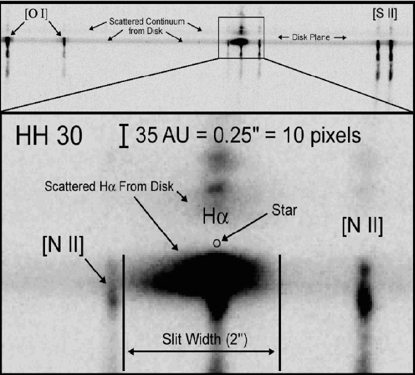
Figure 1: Spectral images of the HH 30 system with the G750M grating. The locations of the star, disk plane, and bright emission lines are marked. Reflected light is present at the top and the bottom of the opaque disk, which is nearly edge-on in this object. The brightest (blueshifted) portion of the jet extends below the disk (to the northeast) in this and subsequent figures, while a fainter redshifted counterjet exists above the disk plane (to the southwest). The slit is much wider than the jet, so these data generate an image for each emission line.

The slit was 52 arcseconds in length and aligned at PA $-$147.35^∘ to lie along the HH 30 jet. With the exception of one set of images taken through the 0.2 arcsecond slit to check for internal velocity dispersion (see below), all data were taken through the 2 arcsecond wide slit. We performed a blind offset from a nearby star to center HH 30 in the slit. The closest star suitable for this offset was over 2 arcminutes away, which could introduce pointing errors of a few tenths of an arcsecond. However, these errors are small compared with the size of the slit, and observations of the scattered light in the disk show that the slit was centered on the source to within $\sim$ 0.2 arcseconds. The C-shaped reflection nebula that surrounds HH 30 extends about 2.5 arcseconds perpendicular to the slit, and therefore fits almost entirely within the slit. Because the nebula also reflects emission lines, an image of the reflection nebula appears near the base of the jet for each of the strong emission lines. Figure 1 shows a portion of the G750M spectrum.

Observations of jets taken through slits that are wider than the jet produce emission-line images at each line, provided the internal velocity dispersion of the emitting gas is unresolved. In our case the slit is $\sim$ 5 times wider than the jet (Fig. 1). Internal velocity widths within HH jets are nearly always $\lesssim$ 100 km s^-1, and are unresolved with the low resolution gratings G430L and G750L. However, we require the medium-resolution grating G750M to image lines separated by 10 $-$ 20 Å, such as [S II]$\lambda$6716 and [S II]$\lambda$6731, and [N II]$\lambda$6583 and H$\alpha$. With most jets, wide slit observations with G750M would be difficult or impossible to interpret because spatial and spectral information are mixed. However, HH 30 lies nearly in the plane of the sky (Wood et al., 2000), and has no strong bow shocks near the source that splatter material along the line of sight. Hence, emission-line velocities and widths in the jet near the star are low. Appenzeller et al. (2005) found that while scattered light generated a weak emission tail that extends to $\sim$ 100 km s^-1 in the spectrum of the disk of HH 30, this emission is down in flux by a factor of $\sim$ 100 from that of the jet, where the emission-line profile lies entirely within a 40 km s^-1 interval. Coude spectra by Mundt et al. (1990) also show narrow line widths in the jet close to the star. An emission-line point source will be imaged over $\sim$ 2.5 pixels in the dithered 750M observations, corresponding to $\sim$ 0.7Å, or $\sim$ 40 km s^-1, so the jet knots should be unresolved in our spectra. To check this, we also imaged the jet with the 0.2 arcsecond slit, and found the emission lines to be unresolved. As a further check, the G750L and G750M emission-line images of well-separated lines such as [O I] 6300 and [O I] 6363 are identical, which demonstrates that the jet is unresolved spectrally in both gratings.

To create an image of a particular line, we simply extract a box centered on that line. It is straightforward to measure the continuum from the reflection nebula on either side of the emission line and subtract it from the image (e.g. Hartigan et al., 2004). Images in various emission lines appear in Figure 2. The relative positions in the x-direction (perpendicular to the jet) are in principle fixed by the wavelength solution. However, the scatter in that solution of $\pm$ 0.3 pixels is improved by a factor of $\sim$ 2 by shifting the x-positions of the images to align the brightest knot in the jet. The jet knot used for alignment appears fairly symmetrical in all the lines, so the uncertainty in its x-position is $\sim$ 0.1 pixel.

Aligning each emission-line image in the y-direction (along the jet) is more involved because the star in HH 30 is not visible, no other stars lie along the slit, and emission lines have offsets from one another in the y-direction owing to heating and cooling along the flow. Fortunately, HH 30 has a bright reflection nebula visible on either side of the disk, which appears as a dark lane in images of the source (Watson & Stapelfeldt, 2004), and it is easy to measure the position of this lane in our spectral images.

At our request, K. Wood and M. O’Sullivan generated a series of 1D slices of a model of the HH 30 reflected light at several wavelengths between 3000Å and 9500Å. The model slices are perpendicular to the disk through a 2-arcsecond slit, and show that the location of the minimum of the reflection nebula at all wavelengths remains fixed to within a half pixel relative to the projected location of the star. The models show that the star is located 0.092 $\pm$ 0.010 arcseconds away from the minimum of the reflected light. We measured the y-location of the minimum of the reflection nebula adjacent to each emission line, and shifted each image accordingly.

Spectra extracted from the flux-calibrated surface brightness images or ratios between sections of such images must be corrected for the point-spread function (PSF) of STIS, which worsens at the reddest wavelengths. The calibration is accomplished with a photometric correction table. The values affect the relative line ratios by $\lesssim$ 10% for wavelengths $<$ 8500Å, which includes all of our lines except for the [C I] 9850 doublet, where the correction is $\sim$ 40%.

3 RESULTS

3.1 Reflection Nebula

The reflection nebula at the base of the HH 30 jet has been known for many years and has been the subject of several investigations. Most recent studies make use of HST observations at optical (B96, Watson & Stapelfeldt, 2004) and near-infrared (Cotera et al., 2001) wavelengths to understand the scattering properties and spatial distribution of the dust. The surface brightness of the nebula varies by as much as 1.5 magnitudes at optical wavelengths, and there is evidence that reflected light from hot spots on the stellar surface causes most of the observed asymmetries in the nebula (Wood & Whitney, 1998; Watson & Stapelfeldt, 2004). Further support for this idea comes from observations of emission lines in the nebula, which have broad velocity tails that are likely to be scattered light (Appenzeller et al., 2005).

The reflection nebula is easiest to study in the low-resolution (G430L and G750L) data because the signal-to-noise in the continuum is higher than it is for the medium-resolution data. A single emission line reflected from the disk appears in the slitless data as an image of the disk in that line, and occurs at some level in all the bright lines in Figure 2, but is especially bright in the Balmer lines, which come in part from the star. Each row of the slitless images that crosses the disk (the jet lies along the columns) provides a spectrum of the reflected light that falls along that row, although all absorption and emission lines will appear broadened by the physical size of the disk in the extracted spectrum. One can obtain an integrated spectrum over a portion of the disk by simply summing the appropriate range of rows.

Spectra of the entire disk show that the total flux of the reflected continuum varies by over a magnitude at V, consistent with previously published results. The blue spectra from 13 August 2000 and 3 September 2000 (Table 1) are nearly identical, so we combined them into a single epoch. The nebula became fainter in the second epoch of blue data (18 August 2002) by a factor that increases steadily from about 2.0 at 3500Å, to 3.0 at 5500Å (Fig. 3). A strong Balmer jump and many emission lines are present in the blue spectra. The red spectrum taken 25 October 2000 was intermediate in flux between the two blue spectra in the region where the wavelengths overlap.

The emission-line images in Fig. 2 show that the broad base to the emission-line profiles in Fig. 3 come from the disk, while the narrow cores arise in the jet. The ratio of the broad to narrow components, measured from the medium-resolution red spectra (the lines are not blended there), is about 0.9 for all the forbidden lines and $\sim$ 4 for H$\alpha$. Both the forbidden lines and Balmer lines from the disk are likely to be scattered light, with the star being the primary source of illumination for the Balmer lines and the jet the primary source for the forbidden lines.

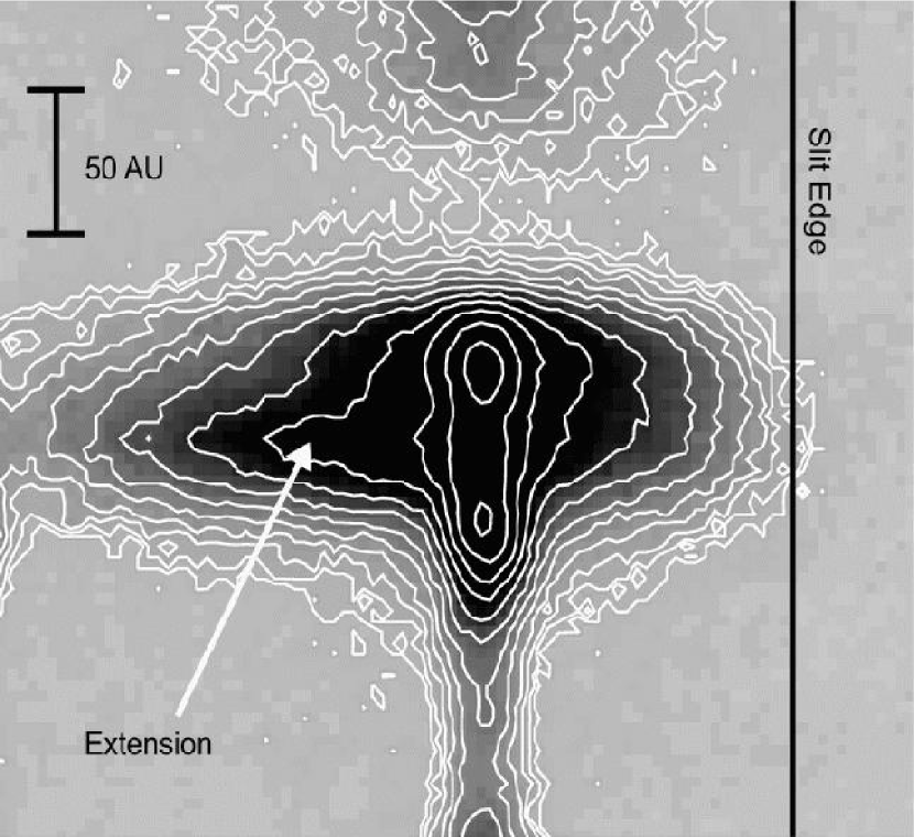
Figure 4: An H$\alpha$ image of the HH 30 disk and jet taken with the G750M grating on 25 Oct, 2000. The disk appears in scattered light, and has a bright extension to the left. The slit partially truncates the disk on the right side. Adjacent contours are separated by a factor of $\sqrt{2}$, and the lowest contour is $2.2\times 10^{-15}$ erg cm^-2s^-1arcsec^-2.

The H$\alpha$ image of the disk in Fig. 4 shows an asymmetry that appears in both epochs of the G750M data, with the H$\alpha$ brighter on the left (northwest). The asymmetry persists in the G750L images, and so is not caused by spectrally resolved scattered blueshifted emission from the outflow. The asymmetry is not present in the forbidden lines, indicating that it originates in the strong H$\alpha$ emitting region in the vicinity of the star. Watson & Stapelfeldt (2004) noted similar asymmetries and attributed them to hot spots on the stellar photosphere caused by accretion columns from the circumstellar disk. The H$\alpha$ scattered light images appear truncated on the right (southeast), but this position likely marks the edge of the slit, because this truncation appears in the forbidden lines as well.

In addition to the Balmer jump and emission lines, there are weak TiO absorption bands at 7800Å and 7100Å in the disk spectrum (Fig. 2, see also Appenzeller et al., 2005), but the signal-to-noise is too low to constrain the spectral type of the star well. Using a STIS spectrum of the M3.5 weak-line T Tauri star HBC 358 (Hartigan & Kenyon, 2003) as a photospheric template, the veiling is about 4 at these wavelengths, while the K7 wTTS Lk Ca7 (primary) gives a veiling of 1.5. By chance, the brightness of the nebula in epoch 1 agrees to within a few tenths of a magnitude with the broadband V and I magnitudes reported by B96.

Watson & Stapelfeldt (2004) found that HH 30’s reflection nebula became bluer further out in the disk, and we also see this effect in our data. The ratio of the G430L spectrum of the outer half ($\sim$ 1/3 arcsecond) of the blueshifted reflection nebula to a spectrum of the inner half (closest to the star) rises in a nearly linear fashion from $\sim$ 1.0 at 5500Å to $\sim$ 1.3 at 3500Å.

3.2 Proper Motions

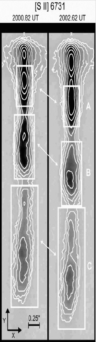
Figure 5: Proper motions in the blueshifted component of the HH 30 jet. The objects labeled A, B, and C move $\sim$ 0.4 arcseconds (56 AU) over a time interval of 1.8 years. Contours are spaced by a factor of $\sqrt{3}$ in these [S II] images, with the lowest contour $1.1\times 10^{-15}$ erg cm^-2s^-1arcsec^-2. The source position is denoted with an ‘X’. A new knot is also emerging from the source.

Knots in the blueshifted (northeastern) half of the HH 30 jet exhibited substantial proper motions of $\sim$ 15 pixels in the 1.8 years between epoch 1 and epoch 2. To measure these motions we combined the continuum-free images of the five brightest forbidden lines visible in the G750M spectra $-$ [O I] 6300, [O I] 6363, [N II] 6583, [S II] 6716, and [S II] 6731 $-$ into a single image for both epochs. We then used the code described in Hartigan et al. (2001) to measure proper motions. The results appear in Table 2 and in Figure 5. Velocities in the blueshifted jet are rather low for an HH jet, $\sim$ 130 km s^-1. Velocity differences of $\sim$ 30 km s^-1 are present, similar to those observed in other HH flows (e.g., Hartigan et al., 2001).

Velocities of knots in the redshifted counterjet are higher than they are in the main, blueshifted jet. Three knots are present in the first epoch at distances of 0.63, 0.96, and 2.38 arcseconds from the star, which we label D, E, and F, respectively. Knots E and F both have proper motions of $\sim$ 225 km s^-1. The motion for knot D is less certain because knots exist in epoch 2 at distances 1.04 and 0.68 arcseconds from the star. Assuming the outer knot is knot D, the proper motion is $\sim$ 150 km s^-1. It is possible that knot D had not emerged fully from the high extinction region of the disk plane in epoch 1, which would result in a lower proper motion for this object. In any event, the redshifted portion of the flow is $\sim$ 1.7 times faster than its blueshifted counterpart. Having one side of a flow much faster than the other side is not unusual for stellar jets (e.g., RW Aur; Lopez-Martin et al., 2003). However, in the case of HH 30 it does not appear that the knots were ejected at the same time (Table 2). There are knots in the HH 30 blueshifted jet at larger distances from the source than knot C in Fig. 5, but these are either partially or completely excluded by our slit because the jet curves at larger distances. The jet appears slightly tilted by about 2 degrees with respect to the position of the slit, and the motions of the knots all lie along the axis of the jet to within the uncertainties of the observations.

It is instructive to compare our results with previous proper-motion measurements. B96 determined proper motions in HH 30 with WFPC2 from broadband red images separated by about a year. While HST can easily detect proper motions over this time interval, the B96 measurements have large errors because the first epoch exposure in particular was not very deep, and the images include bright continuum from the disk which makes it more difficult to measure accurate positions for knots within an arcsecond of the star. Proper motions of the six knots in the blueshifted jet measured by B96 have a large scatter, from as low as 54 km s^-1 to as high as 258 km s^-1, with an average of 142 km s^-1. Ground-based images do not resolve individual knots well close to the source, but Mundt et al. (1990) measured 170 $\pm$ 50 km s^-1 for the proper motion of a distant knot $\sim$ 10 arcsesconds from the star.

The combination of deep exposures (10 $-$ 30 ksec), a factor of four smaller pixel scale in the dithered STIS images compared with WFPC2, precise continuum subtraction, and improved analysis software greatly reduces the errors in the proper motions to $\pm$ 4 km s^-1. With this precision it is possible to distinguish real velocity differences between adjacent knots and to predict where the features we observe now should have appeared in the January 1995 images of B96 (the spatial resolution is too low in the ground-based images to make a useful comparison). The knot labeled ‘A’ in the blueshifted jet in Fig. 5 was ejected after 1995, but knot ‘B’ should have been located at a distance of 0.40 $\pm$ 0.03 arcseconds from the star in January of 1995. This position corresponds reasonably well, given the uncertainty of the source position and the different filter used, with knot 9501-N, which B96 reported at a distance of 0.51 arcseconds. However, the B96 tangential velocity of only 54 km s^-1 is much lower than our value of 149 $\pm$ 4 km s^-1 (Table 2). The difference may be caused by uncertainties in measuring proper motions within the reflected light cavity of the disk with the broadband B96 images.

Our object ‘C’, which we measure as having a proper motion of 125 $\pm$ 4 km s^-1, should have been located 2.11 $\pm$ 0.03 arcseconds from the star in January 1995. B96 report three knots in this area, 9502-N (1.1 arcseconds, 258 km s^-1), 9503-N (2.0 arcseconds, 158 km s^-1), and 9504-N (2.7 arcseconds, 84 km s^-1). It appears that these three objects visible in 1995 have now merged into a single structure – object C extends for $\sim$ 1.8 arcseconds, about the distance between 9502-N and 9504-N in 1995.

Some structural changes are evident in Fig. 5. Knot A became more elongated between 2000 and 2002, while knot B widened and faded, and the portion of knot C closest to the star also faded somewhat. These changes are likely caused by internal motions, shocks, rarefactions and cooling still unresolved in these images. However, internal motions in these knots cannot exceed $\sim$ 40 km s^-1 to remain consistent with observations of narrow intrinsic linewidths in these knots. A new knot (labeled ‘N’ in Figs. 6 and 7) was emerging from the source during our observations, but proper-motion measurements are not possible because the feature has not yet detached clearly from the source.

3.3 Jet Collimation

The factor of four finer spatial scale of our dithered slitless STIS images relative to narrowband WFPC2 images, the lack of continuum, better hot pixel removal strategies, and long exposure times create an unprecedented database for measuring the width of the HH 30 jet. The best images for this measurement are [S II] 6716 and [S II] 6731 with G750M, and [O I] 6300 with G750M and G750L, because in each of these cases the lines are bright and unblended, and there is no stellar emission-line component. We measured the FWHM by extracting spatial profiles every three pixels along the jet in each emission-line image and fitting a Gaussian to the profile with the SPLOT command in IRAF. Errors are dominated by uncertainties in the baseline, and are larger near the star where the disk reflects the line emission in the jet. The instrumental FWHM for slitless observations is that of the PSF of STIS. We used the experimentally measured values and uncertainties of the PSF reported in Hartigan et al. (2004) to deconvolve the FWHM, and propagated the errors of the measured FWHM with the uncertainties in the deconvolution kernel to obtain errors for each deconvolved point.

Results are shown in Fig. 6 for epoch 1, which have both G750L and G750M data, and in Fig. 7 for epoch 2. The widths measured from the G750L and G750M exposures in [O I] 6300 are identical, so the jet is unresolved spectrally in all images. The upturn in the linewidth for the [O I] points $\lesssim$ 15 AU is likely to be instrumental in origin. The brightness of the jet drops sharply inside 20 AU, implying less contrast with the reflected emission lines in the disk. Also, there will be some light in the wings of the PSF from the bright jet at $\gtrsim$ 30 AU that contaminates these measurements.

The collimation properties of the HH 30 jet have been the subject of some debate in the literature. Using HST, B96 observed an opening angle of about 3 degrees, and measured the width of the jet to within about 70 AU of the star. They concluded that the jet was unresolved at this distance, with a FWHM $\lesssim$ 20 AU. In contrast, Ray et al. (1996) analyzed the same image and found the jet to be spatially resolved everywhere, with a FWHM $\sim$ 35 AU at a distance of 50 AU from the star, implying a very wide opening angle for the jet at the source. Deconvolving ground-based images with an FFT algorithm, Mundt et al. (1991) reported an even larger FWHM of $\sim$ 60 AU at a distance of $\sim$ 350 AU, although this measurement is very difficult to do because the jet is much narrower than the seeing disk (which is $\sim$ 1 arcsecond or 140 AU FWHM).

Our new observations settle this controversy. Fig. 6 shows that the jet is indeed spatially resolved everywhere by at least 5$\sigma$, though the width is only about half that reported by Ray et al. (1996) and by Mundt et al. (1991), and is near the upper limit of B96. The jet widens gradually from 14 $\pm$ 3 AU at 20 AU from the source to 36 $\pm$ 4 AU at 500 AU, implying an opening half-angle of 2.6 $\pm$ 0.4 degrees, consistent with the opening angle determined by B96 at larger distances.

The HH 30 jet is similar to other jets (e.g. Hartigan et al., 2004) in that it does not project to a point at the source. However, this observation does not mean that the jet emerges from a disk of radius 14 AU. Rather it is more likely that the opening angle of the flow is wider near the source, as expected for a wind launched from an accretion disk. There is no obvious correlation between the presence of a bright knot and the width of the jet, as also noted by Ray et al. (1996). However, there is some structure in the width of the jet, including relatively wide areas at about 230 AU and 310 AU during epoch 1 (Fig. 6). These areas propagated downstream about 50 AU by epoch 2 (Fig. 7), at about the jet velocity. Apparently these sort of irregularities in the jet develop near the source and the flow simply carries them along (see also Fig. 5).

On the fainter, redshifted side we coadded all the forbidden lines together to improve the signal-to-noise but we were only able to measure jet widths within $\sim$ 400 AU of the star (Fig. 8). The measurements are too uncertain to constrain the opening angle well, but the jet is clearly resolved everywhere and is wider than it is on the blueshifted side. At larger distances from the star, previous images of the region (Mundt et al., 1990, 1991, ; B96) have also shown that the redshifted flow is wider and has a larger opening angle than its blueshifted counterpart. Being able to compare the opening angles, velocities, and widths in both a jet and a counterjet is a potentially powerful diagnostic tool for analyzing the physics of how jets are launched provided enough sources can be observed to derive meaningful statistics.

For a freely expanding flow, the observed opening half-angle corresponds to a Mach number of 21.8. Using a jet velocity of 130 km s^-1 we find a sound speed of 6.0 km s^-1, which corresponds to a temperature of only 2600 K for a ratio of specific heats $\gamma$ = 5/3 and mean molecular weight 1. This temperature is far too low to explain the fluxes in bright lines that originate from upper levels such as [S II] 4068. The more likely value is $\sim$ 10 km s^-1, which should occur for low-excitation forbidden lines in a mostly neutral cooling zone of a shock.

The observed opening angle is consistent with the temperature if there is a source of confining pressure that is on the order of the thermal pressure. The pressure cannot be provided by an ambient external medium, because shear between the jet and this medium would rapidly heat the interface between the two fluids, creating strong shock waves in each that do not appear in the observations. Instead, the most likely candidate for a confining pressure is a toroidal magnetic field. Equating the magnetic pressure with the thermal pressure, using a total density of $10^{6}$ cm^-3, and sound speed of 10 km s^-1 (T = 7260 K) we find the magnetic field B $\sim$ 5 mG at $\sim$ 300 AU, in agreement with the ‘fiducial’ values of field strengths in jets at this distance discussed by Hartigan et al. (2007).

3.4 Emission Line Ratios within Individual Jet Knots

Fig. 9 shows the observed ratio images of the four bright, red forbidden lines for the two epochs. The signal-to-noise is excellent in the ratio images, with uncertainties in the ratios of $<$ 5% except within $\sim$ 50 AU of the source at the edges of the jet, where reflected light introduces higher uncertainties. The effect of scattered light is highest on the blue (left) side of the ratio images that involve [N II] 6583, because scattered H$\alpha$ from the disk contaminates that side of the emission-line image. The images were registered to the stellar position (marked with a horizontal white line) as described in section 3.1. The shorter horizontal lines in the figure mark locations of bright knots N, A, B, and C in the summed forbidden line images for each epoch, and are included as guides.

The easiest emission-line ratio to interpret is that of [S II] 6716/[S II] 6731, which decreases monotonically with increasing electron density. This ratio image clearly shows that the electron density increases close to the source (see also Bacciotti et al., 1999), although the ratio is in the high density limit close to the star and therefore only gives a lower limit to the electron density in those areas. The [S II] ratio image also shows that the density declines near the edges of the jet. This decline has been inferred from STIS mapping in other jets (e.g. Bacciotti et al., 2000), but Fig. 9 shows the effect with unprecedented spatial resolution and clarity. The intensities in the combined forbidden line images in the two left panels are far more concentrated along axis than is the electron density. Two effects contribute to this behavior: first, the volume emissivity is proportional to n² so small density fluctuations translate into larger flux variations; and second, the brightness in the emission-line images integrates along the line of sight, making the jet appear brighter along its axis even for a uniform density cylinder.

The second set of image ratios in Fig. 9 is [N II] 6583/[S II] 6716+6731. This ratio depends primarily on the ionization fraction, but also has a weak positive dependence on both the electron density and temperature. Hence, this ratio follows ‘excitation’ such as shocks, increasing wherever the gas becomes hotter, denser, and more ionized. The N II/S II ratio images from the two epochs are fascinating, and show substructure not apparent in the individual images. The ratio is high in the two bright knots A and B, and these high excitation regions move outward with the flow velocity. The highest excitation portions of the jet lie closer to the source than the brightest portions of the knots in both cases. Additional structure in this ratio appears in the second epoch in the vicinity of knot N.

There is a region of relatively low [N II]/[S II] near the source, also present in the [N II]$\lambda$6583/[O I]$\lambda$6300 ratio (not shown). This decrease appears to be real and not instrumental. A registration error along the jet of 2 pixels between the two images would produce a similar falloff of [N II]/[S II] near the source, but the reflected light profiles in the original images show that registration uncertainties are at most 0.5 pixels. As a final check, the [N I]$\lambda$5199+5201/[N II]$\lambda$6583 ratio also rises $<$ 30 AU from the source, indicating that a drop in ionization fraction occurs there (see next section). Beyond knot B, the [N II]/[S II] ratio declines as noted by Bacciotti et al. (1999).

The final ratio shown in Fig. 9 is [O I]$\lambda$6300/[S II]$\lambda$6716+6731, which is primarily sensitive to density, although the [O I]$\lambda$6300 line also has a positive dependence on temperature not present in the [S II] lines because the collision strength of [O I] is a function of temperature. In a mostly neutral plasma like a stellar jet, most oxygen is O I, and essentially all sulfur is S II. The upper levels for the [O I]$\lambda$6300 and [S II]$\lambda$6716+6731 transitions have similar energies so the temperature dependence of the ratio is weak. However, the critical density of [O I]$\lambda$6300 ($\sim 10^{6}$ cm^-3) is significantly higher than that for [S II]$\lambda$6716+6731 ($\sim 10^{4}$ cm^-3), so [O I]$\lambda$6300 becomes stronger relative to [S II]$\lambda$6716+6731 close to the star where the density is high. Comparing the [S II]$\lambda$6716/[S II]$\lambda$6731 ratio image with [O I]$\lambda$6300/[S II]$\lambda$6716+6731 shows that the latter ratio increases sharply as the S II lines approach the high density limit, so together these three emission lines constrain the density well everywhere in the jet.

4 Discussion

4.1 Physical Conditions Along the HH 30 Jet

A main motivation of this work is to convert images of emission-line ratios like those in Fig. 9 to images of T_e, N_e and X_H = N_HII/(N_HII+N_HI) at each epoch. In this section we describe how to create these images, consider how these variables change along and perpendicular to the jet, and investigate the sensitivity of results to assumptions such as abundance values and charge exchange coupling. The results give the first clear picture of how jets are heated as they emerge from their sources. Our data can also be used to infer the reddening and mass loss rates but we defer discussion of these issues to a second paper, where we also include blended blue doublets such as [S II]$\lambda$4068+4076 and [O II]$\lambda$3727+3729 into the analysis.

4.1.1 Determination of T_e, N_e, and X_H

We use images of the four brightest forbidden lines obtained with the G750M setting, [O I]$\lambda$6300, [N II]$\lambda$6583, [S II]$\lambda$6716, and [S II]$\lambda$6731, to find T_e, N_e, and X_H at each point in the jet where the S/N in the ratio between any pair of these lines is $\gtrsim$ 5. N I, N II, O I, O II, and S II each have five levels populated in nebular conditions: ³P, ¹D, ¹S for O I and N II and ⁴S, ²D, ²P for O II, N I, and S II. We do not use [O I]$\lambda$6363 or [N II]$\lambda$6548 for anything other than flux calibration. Ratios of [O I]$\lambda$6363 / [O I]$\lambda$6300 and [N II]$\lambda$6548 / [N II]$\lambda$6583 are constant to within the errors of measurement everywhere along the jet, and equal the ratios of their respective A-values, as expected from lines that originate from a common upper level. The other bright red line in the HH 30 jet is H$\alpha$, but this line has a prominent reflected stellar component that contaminates the jet emission.

We constructed a model level population for N I, N II, O I, O II, and S II for a grid of N_e and T_e with the atomic parameters summarized in Appendix B. With solar-like abundances (O=8.82, N=7.96, S=7.30 on a log scale with H=12.0) we calculated emission-line ratios for X_H = 0 $-$ 1 in increments of 0.01, log N_e = 2 $-$ 7 in steps of 0.1, and T_e/$10^{4}$K = 5 $-$ 25 in steps of 0.5 assuming the ionization of N and O are tied to H by charge exchange as described below, and all S is S II. The latter assumption makes sense as no [S III] or [S I] lines are present in the spectrum. The best fit physical parameters were defined at each point by minimizing the quadratic form C described in Appendix A over this grid of 209100 models (100$\times$51$\times$41).

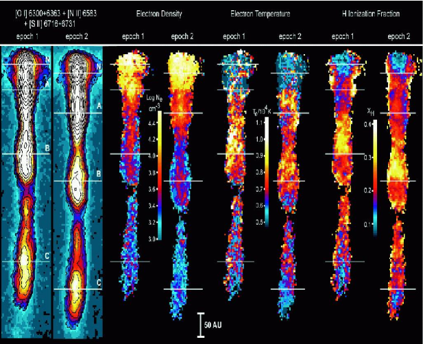
Figure 10: Same as Fig. 9 but for the electron temperature, electron density and hydrogen ionization fraction X_H = H II/(H I+H II). The area of high excitation (high X_H and T_e, color coded as yellow and white) in knot B moves outward with the flow. The jet emerges with a very low ($\lesssim$ 0.1) ionization fraction, and becomes more ionized beyond $\sim$ 50 AU. At large distances the ionization declines.

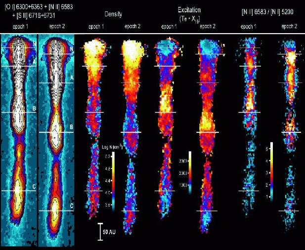
Figure 11: Same as Figure 9 but for the total density, excitation, and [N II] 6583/[N I] 5200 ratio. The total density rises to a value of $\sim$ $4\times 10^{5}$ near the source, and is higher (red and yellow colors) in the bright knots and along the axis of the jet. Dense filaments, most easily seen in the epoch 2 image, are present within knot B. The excitation image, created by the product of the ionization fraction and the electron temperature, shows several areas of heating between $\sim$ 50 AU and 500 AU from the star. The [N II]/[N I] ratio, which is not dereddened, declines close to the source even though the density and reddening both increase toward the source, and both factors act to increase the ratio. The only explanation for the decline of the ratio close to the source is that the jet is more neutral there, in agreement with the ionization map in Figure 10.

The resulting images of N_e, T_e and X_H appear for each epoch in Fig. 10, where, as in Fig. 9, the horizontal white line marks the location of the star and short white lines denote the position of the knots in the jet at each epoch. Dividing the electron density by X_H produces a total density image, and the product of T_e and X_H gives an ‘excitation’ image that is sensitive to hot ionized gas, as one should find behind a shock wave (Fig. 11). The density images largely resemble what appears in the [S II] image ratio in Fig. 9, with the dominant behavior the decline of density with distance from the source, as has been observed before at lower spatial resolution in the 1-D plots of Bacciotti et al. (1999). Density measurements are still possible close to the source where the red [S II] lines are in the high density limit because the best fit solution also includes line ratios that involve [O I]$\lambda$6300, which is not in the high density limit.

The decline of the total density with distance shown in Fig. 12 resembles that produced by a radial conical flow that originates from a finite source region. The jet is also a factor of two denser along the axis than it is at its edges, and the bright portions of the jet are typically the densest. The high-density knots clearly move along the jet, and the higher S/N images of the second epoch show what appear to be density filaments at the limit of the spatial resolution in knot B. When interpreting these images one should keep in mind that the observations integrate along the line of sight, which tends to smooth over density gradients in the jet.

The images of X_H and excitation show a rapid rise, followed by a gradual decline with distance from the source (see also Bacciotti et al., 1999). Figs. 11 and 12 show that this variation is not smooth; instead, the high excitation regions show sharp, almost linear boundaries, and move outward with the flow. The regions of high excitation occur on the side of the knot closest to the source for both knots A and B. In knot A we see that this area of high excitation appeared between the first and second epochs, indicating a heating event.

The rise of the ionization/excitation in the first 100 AU as the jet emerges from the source in a series of well-defined heating events is a critical observational result of this paper that affects all models of jet launching, so it is important to verify that the result does not depend upon the emission-line ratios used in the analysis. As noted above, using other lines close to the source typically requires reddening corrections, but in this case we can use the G430L [N I]$\lambda$5199+5200 image to confirm the low value of X_H found close to the source from the red line ratios. If the ionization fraction remained constant, the [N II]$\lambda$6583 / [N I]$\lambda$5199+5201 ratio should increase steadily towards the source because the critical density of [N II]$\lambda$6583 exceeds that of [N I]$\lambda$5199+5201, and because the reddening increases toward the source. However, images of this ratio in the last panel of Fig. 11 clearly show that the ratio is lower close to the source, which can only happen if the ionization fraction is lower there.

4.1.2 Effects of Charge Exchange Coupling, Reddening, and Abundances

The assumption that charge exchange sets the ionization fractions of O and N given the ionization fraction of H is worth investigating further, as it is required to solve for the hydrogen ionization fraction and temperature from a database that consists of only [N II]$\lambda$6583, [O I]$\lambda$6300, [S II]$\lambda$6716, and [S II]$\lambda$6731. The charge exchange cross section between H and O is large and has almost no temperature dependence because the ionization energies of H and O are nearly the same. However, the charge exchange cross section is three orders of magnitude lower for H-N than it is for H-O, so there is some question as to how well the ionization fractions of N are tied to those of H, especially since the ionization potentials of H and N differ by $\sim$ 0.9eV. Bacciotti & Eislöffel (1999) argue that the H-N charge exchange rate is high enough to fix the (H I/H II)/(N I/N II) ratio as long as the hydrogen ionization fraction is $\lesssim$ 50%, but their model did not include photoionization, which affects H and N differently owing to the different ionization potentials.

To test the validity of H-N charge exchange coupling we created a time-dependent photoionization model, varying the ionizing spectrum and strength, and included the atomic physics of collisional ionization, recombination, dielectronic recombination, photoionization and charge exchange (see Appendix B for references) to determine how closely the ionization fraction ratios of H and N follow those predicted by charge exchange coupling.

The first case we tested was to singly ionize all the H, N, and O, and follow the ionization fractions as the gas recombined. As expected, the (H I/H II)/(O I/O II) ratio approached rapidly to the value predicted from charge exchange (to within 1 part in $10^{4}$ after 0.1 $\tau_{REC}(H)$, where $\tau_{REC}(H)$ is the H recombination timescale), and remained equal to the charge exchange ratio as the gas recombined. The ionization fraction of N was 10% lower than the charge exchange value after 0.5 $\tau_{REC}(H)$ improving to 5% lower after 2 $\tau_{REC}(H)$. Experiments with input blackbody photoionizing spectra yield similar results as long as the ionization fraction of H is $\lesssim$ 90%. Even the extreme case where the photoionizing flux is low and H starts out completely ionized with N completely neutral (so that charge exchange is solely responsible for ionizing N) equilibrates to within $\sim$ 20% of the charge exchange prediction after one $\tau_{REC}(H)$. We conclude that the H-N charge exchange coupling assumption is well-justified.

Another issue is whether or not we should attempt to deredden the fluxes of the four emission lines. In principle one might use the Balmer decrement (H$\alpha$/H$\beta$) for this purpose. The observed Balmer decrement in the bright knots varies between about 3.0 and 3.5, and rises to $\gtrsim$ 5 in the reflection nebula and between the bright knots. This variation of the Balmer decrement is likely to be caused by differing decrements in the scattered light from the star and the intrinsic emission from the jet. Hence, we cannot use the decrement directly to find the reddening, and instead must incorporate various blue doublets such as [O II]$\lambda$3727+3729, [S II]$\lambda$4068+4076, and [N I]$\lambda$5199+5201 into the analysis. We defer this work to a subsequent paper. The Balmer decrement in the bright jet knots indicates that A_V $\lesssim$ 1, so differential reddening between [O I]$\lambda$6300 and [S II]$\lambda$6731 is a factor of $\lesssim$ 1.04, and between [N II]$\lambda$6583 and [S II]$\lambda$6731 a factor of $\lesssim$ 1.02, small compared with the uncertainties in the relative abundances of O, N, and S in the Taurus star forming region. We ignore these small effects of differential reddening for the current analysis.

The density maps are largely independent of the abundances because the [S II]$\lambda$6716/[S II]$\lambda$6731 ratio strongly constrains N_e when log N_e $\lesssim$ 4. For a fixed set of observed emission-line ratios, reducing the nitrogen abundance by a factor of two increases X_H by a factor of 1.8 and T_e by a factor of 1.2. Overall, the fit to the line ratios becomes worse for about 3/4 of the pixels and better for the remaining 1/4. Hence, it is possible to constrain abundances with these data but the uncertainties are relatively high. We also defer this analysis to a subsequent paper.

5 Implications for Jet Heating

The images presented in Figs. 9 $-$ 11 provide the best information to date concerning how jets are heated as they emerge from their sources. The observations show that some process heats and partially ionizes the jet from $\lesssim$ 10% within $\sim$ 20 AU of the star to as high as 30% -40% at $\sim$ 100 AU from the star. The ionization increase is not a steady process, but instead produces relatively sharp boundaries, and areas of high ionization move outward with the flow velocity. The heating is not caused by photoionization from the source, because the ionization fraction is initially low close to the source, and increases outward. Similarly, a stationary focusing shock in the jet does not explain why the jet produces distinct knots with relatively high ionization fractions, and there is no indication of any narrowing in the jet that should accompany such a shock.

The most obvious candidates for heating and partially ionizing the flow are shock waves produced by supersonic variations in the flow velocity. This scenario explains why the jets are heated at some distance from the source, and internal shocks produce sharp ionization features that propagate with the flow velocity, in agreement with the observations. However, one important aspect of the data does not fit this model $-$ the density should increase substantially in the postshock regions where the excitation is high, and it does not.

It may be possible to produce sharp rises in the ionization fraction without increasing the density substantially if the shocks are magnetic. In this case the postshock pressure is dominated by the magnetic field, and relaxes on the timescale for Alfven wave propagation, while the ionization in the shocked region relaxes on the recombination timescale. Non-steady MHD jet models with atomic physics accurate enough to follow ionization fractions have not yet been done, but the ionization signature of a supersonic magnetic collision should linger substantially longer than the density enhancement does in stellar jets. Magnetic field strengths in jets at distances of $\sim$ 100 AU from the source are poorly understood, but recent models of time-dependent MHD pulses indicate that the Alfven velocity could be $\gtrsim$ 50 km/s in these regions (Hartigan et al., 2007), so an Alfven wave would cross the jet on a timescale of $\lesssim$ 2 years. In comparison, the recombination time for H gas with a density of $10^{4}$ cm^-3 is longer, $\sim$ 10 years, approximately equal to the flow time from knot A to knot C.

The general decline of ionization with distance means that more heating events occur close to the star (as expected for stochastic velocity perturbations). Beyond $\sim$ 1000 AU from the star, proper-motion measurements and high-resolution HST images of jets (e.g. Hartigan et al., 2001; Heathcote et al., 1996) show that jets are heated by internal shock waves. At these distances, small velocity perturbations have washed out, so the jet gradually recombines and remains mostly neutral and cool until it encounters a major working surface.

6 SUMMARY

We have constructed deep optical emission-line images of the HH 30 stellar jet using STIS spectroscopy taken through a wide slit. The system has a fortunate geometry, with the axis of the jet nearly in the plane of the sky. Hence, it is possible to observe the jet without projection effects and we can trace the flow to within $\sim$ 20 AU of the star. Low radial-velocity dispersions within the flow mean that the STIS spectra are effectively slitless, and produce images for each emission line, including those for which HST has no narrowband filters. The resulting data set, dithered for maximum spatial resolution and observed at two epochs, enables us to diagnose physical conditions in the region where the jet first emerges from the accretion disk.

Individual knots in the HH 30 jet show distinct proper motions between the 1.8 years that separate the two epochs. Motions in the blueshifted jet range from 116 km s^-1 to 149 km s^-1, with uncertainties of $\pm$ 4 km s^-1. The jet has a resolved spatial width of FWHM $\sim$ 14 AU at a distance of 20 AU from the source, and has a constant opening half-angle of 2.6 degrees. The narrow opening angle is consistent with the observed velocity and sound speed if there is an additional confining magnetic pressure from toroidal fields in the jet. Velocities in the redshifted counterjet are $\sim$ 100 km s^-1 higher than they are in the main jet, and the counterjet is less well-collimated than the main jet.

Spectra of the reflected light from the HH 30 disk reveal a veiled, late-type photosphere with both permitted and forbidden emission lines and a prominent Balmer emission jump. The reflected light from the disk varies substantially in both morphology and in brightness, and is bluer at larger distances from the star.

We developed a new analysis technique to find the best fit for the electron temperature T_e, electron density N_e, and hydrogen ionization fraction X_H given a set of observed and model emission-line ratios. The method, based on minimizing a quadratic form, has the advantage that by construction it uses all the information present in each available line ratio, and appropriately weights the fit of each ratio by the uncertainty.

Our analysis focused on six ratios involving the four bright nebular lines of [N II]$\lambda$6583, [O I]$\lambda$6300, [S II]$\lambda$6716, and [S II]$\lambda$6731, with additional ratios using [O I]$\lambda$6363, [N II]$\lambda$6548, H$\alpha$, H$\beta$, and [N I]$\lambda$5199+5200 used to verify the results. The images from each epoch produce the first high-resolution images of T_e, N_e and X_H in a stellar jet. The density in the jet is highest close to the source, and declines in a manner similar to that of radial conical flow from a finite source region. The density in the jet is larger by a factor of two along the axis than at its edges. Distinct bright knots are also denser, and propagate at the flow velocity.

Maps of the ionization fraction and excitation (defined as the product of T_e and X_H) show that the jet emerges with an ionization fraction of only $\sim$ 10% , which increases to $\sim$ 30% at $\sim$ 100 AU from the source. Regions of locally higher ionization propagate with the flow, and exhibit sharp spatial boundaries. At least one such knot formed between the two epochs. Surprisingly, the high-excitation knots are not accompanied by a density enhancement, suggesting that they may originate from velocity variability in a highly magnetized flow.

The two epochs reported in this paper were an accidental benefit of a delay in HST scheduling. Stringent ORIENT requirements limited visibility windows for the spacecraft, and NICMOS took priority for all usable 2001 dates. As a result, our data were taken in two narrow time intervals, making it possible to study the motions and variability of the jet and the disk. Stellar jets are dynamical systems, and we must watch them move to be sure we understand the physics that governs them. Because of the two epochs, we now know where the jet is heated and we are beginning to understand the process that causes the heating. Multiple epoch observations with the highest spatial resolution possible are clearly the best way to study these remarkable objects.

7 APPENDIX A: Measuring Electron Densities, Electron Temperatures and Hydrogen Ionization Fractions From Emission Line Ratios

In this appendix we describe our method for extracting electron densities, temperatures, and hydrogen ionization fractions from a set of emission-line ratios and uncertainties. In general, an observed emission-line ratio from an optically thin plasma where the dominant processes are collisional excitation, collisional deexcitation and radiative decay depends on the reddening, the relative abundances of the two elements, their respective ionization fractions, the electron temperature and the electron density. One can use the flux ratio of lines with closely-spaced upper energy levels such as [S II]$\lambda$6716/[S II]$\lambda$6731 to measure the electron density directly, because these ratios are independent of abundances, reddening, and ionization fractions, and insensitive to the electron temperature. This method has been applied to HH objects for at least a half century now (Böhm, 1956). Other line ratios that arise from the same ion but where the upper levels differ markedly in energy (e.g. [O I]$\lambda$5577/[O I]$\lambda$6300]) depend on both the temperature and density, so with the density in hand one can measure the temperature (Brugel et al., 1981; Hartigan et al., 2004).

A variant of the above ideas introduced by Bacciotti & Eislöffel (1999) was to use the additional constraint of strong charge exchange coupling between H and O, and H and N, which ties the H I/H II ratio to O I/O II and to N I/N II given the temperature of the gas. Assuming standard abundance ratios of N/O, O/S and N/S, and taking all the S to be S II, one can then use [S II]$\lambda$6716/[S II]$\lambda$6731 to obtain the electron density as before, and employ [N II]$\lambda$6583/[O I]$\lambda$6300, [S II]$\lambda$6716+6731/[O I]$\lambda$6300, and [O I]$\lambda$6300/[N II]$\lambda$6583 to estimate the temperature and ionization fraction. Because these lines all have similar upper level energies, the temperature determination is the most uncertain, and relies mostly upon the temperature dependence of the collision strength of [O I] for the measurement. The main advantage of assuming that charge exchange ties the ionization fraction of hydrogen to that of nitrogen and oxygen is that one can then estimate the desired physical quantities from bright lines in the less-extincted red part of the spectrum that are close enough in wavelength to make differential reddening corrections negligible.

Estimates of N_e, T_e, and X_H made in this manner implicitly assume that these parameters do not vary substantially over a size scale equal to the spatial resolution of the observations. However, as shown clearly by Brugel et al. (1981), and more recently by Podio et al. (2006), temperatures and densities of HH objects measured with different line ratios produce markedly different results. The reason for this behavior is that HH objects are shock waves. Emission lines from shocks radiate at different places in the cooling zones, with high-excitation lines and lower critical densities more prominent near the front, and low-excitation, high critical density lines stronger at larger distances. Unless the cooling zones are resolved spatially, almost never the case with ground based observations of HH jets, constructing line ratios when the component lines sample different physical conditions can lead to inconsistent results. Hence, great care must be taken when interpreting large scale trends in HH shocks when the cooling zones are unresolved. Fortunately, HST resolves the cooling zones for most knots in jets (Heathcote et al., 1996), so it is possible to apply the above analysis to many such images.

There are several aspects to the above methods of analysis that are less than ideal. The [S II]$\lambda$6716/[S II]$\lambda$6731 ratio is usually in the high density limit close to the source, and provides only a lower limit to the electron density there. Density information is contained in other line ratios, but the analysis does not use all the ratios. Moreover, it is unclear how to incorporate additional line fluxes into the analysis. For example, if in addition to the four lines ([S II]$\lambda$6716, [S II]$\lambda$6731, [N II]$\lambda$6583, and [O I]$\lambda$6300) used by Bacciotti & Eislöffel (1999) we also observe [N I]$\lambda$5199+5201, what is the best way to include this observation in the analysis? In principle, the new observation defines four new emission-line ratios, each with a different uncertainty.

7.1 Definition of the Problem

Given a set of n observed line fluxes F₁,F₂,…F_n, what is the best way to determine the physical parameters N_e, T_e, and X_H = n(H II)/n(H I+H II)?

We begin by discarding the flux normalization. Absolute line flux measurements from ground-based spectra are rather rare, as they require photometric conditions and are complicated by atmospheric dispersion and pointing uncertainties. Physically, the volume of emitting gas along the line of sight and the reddening determine the absolute fluxes for these optically thin lines. In HH jets, which are inherently clumpy, the absolute fluxes determine the volume filling factor of the emitting material if one knows the width of the jet, but the absolute fluxes do not affect estimates of T_e, N_e, and X_H, which depend only upon the flux ratios. Hence, our analysis deals only with flux ratios. The extra step of determining filling factors is easy to add after one finds T_e, N_e, and X_H, assuming the spectra are flux-calibrated.

Most studies present line ratios relative to some normalization, typically H$\beta$ or H$\alpha$ = 100. However, there is no reason a-priori to favor any particular line for the normalization. Consider Table 3, which shows artificial data for two models and an observation of three emission lines, H$\alpha$, [O I]$\lambda$6300 and [N II]$\lambda$6583. At first glance it appears that model B fits the observations better than model A because the [N II] flux is off by a factor of two in both models, but model B gets the [O I] right while model A is again low by a factor of two. However, there is an additional line ratio to consider, which is [O I]/[N II], and model A predicts this ratio correctly while model B is off by a factor of two. Hence, if we consider all line ratios equally, both model A and model B are equally good fits, because they both get one ratio correct and miss the other ratios by factors of two.

7.2 The Quadratic Form C

Motivated by the above discussion, we seek a measure that will use all the emission-line observations in equal, and appropriately weighted manners to determine the best fit set of the parameters N_e, T_e, and X_H. Given n line flux measurements we can construct p = n(n$-$1)/2 distinct pairs. The deviation of the model from the data should be the same for a ratio and for its inverse, and to ensure this behavior we define a new set of p ratios r_k, where r_k = ln(F_i/F_j) for some integers i, j = 1, 2, …, n, with i $<$ j. The most obvious choice to determine a best fit model is to minimize the quadratic form

$$C=\sum_{k=1}^{p}{{\left(r_{k}-m_{k}\right)^{2}}\over{\sigma_{k}^{2}}}$$

where m_k is the model prediction of the line ratio k from a given model, and $\sigma_{k}$ is the observational uncertainty in the line ratio.

The quadratic form C has all the properties we desire for a line ratio fitting algorithm. Each of the emission-line ratios contributes on an equal basis to the value of C according to the uncertainty in the ratio. The best fit is determined from line ratios and not fluxes, and information from each ratio is automatically incorporated into the fit for the best physical parameters. If, for example, ratio r_i is unaffected by the temperature then it will contribute equally to the value of C for all models that differ only in the temperature. Line ratios that give only upper limits will do so in the values of C as well. Adding new emission lines into the analysis is trivial. Applied to models A and B in Table 3, we see that C_A = C_B, as desired. We define the ‘best’ fit to a given set of parameters T_e, N_e, and X_H to be the one that minimizes C for a set of observed line ratios.

7.3 The Probability Distribution of C

An outstanding issue is how one should interpret the values of C. Although this exercise has no bearing on the choice of the best fit, which by definition is the one with the lowest value of C, it is still useful to investigate the probability distribution of C because in a formal sense the values of C determine confidence intervals for rejecting a null hypothesis that the model exactly matches the data.

For astronomical spectra it is reasonable to take the individual r_k to be distributed normally. Equation A1 looks a lot like a $\chi^{2}_{n}$ distribution, but it is not because the r_k are not independent of one another. For example, in Table 3 any two line ratios suffice to determine the third. If m and r are the p-dimensional vectors of a set of model ratios and observations, respectively, and the r_i have a normal distribution with mean m_i and variance $\sigma_{i}^{2}$, then a standard result from multivariate statistics is that the probability density function

$${1\over{\left(2\pi\right)^{p/2}\sqrt{|{\bf V}|}}}exp\left[{-({\bf r}-{\bf m})^{T}{\bf V}^{-1}({\bf r}-{\bf m})}\over{2}\right]$$

is a multivariate normal, where V is the covariance matrix of r, and the superscript ‘T’ denotes a transpose. Using the above notation, the quadratic form H = (r$-$m)^TV^-1(r$-$m) is distributed as a $\chi^{2}_{n}$ (Hoog & Craig, 1995). In the case of independent r_i, the covariance matrix is diagonal and we recover the standard definition of $\chi^{2}_{n}$. While we could also minimize H to find the best fit, with the benefit that H then has a known probability distribution, doing so requires inverting the covariance matrix at each point within an emission-line map, an extra computational step that did not seem warranted given that the quadratic form C exhibits all the properties we desire for a best fit solution to the problem.

The probability distribution of C = x^TAx has been studied thoroughly in the mathematical literature. Examples include independent normal variables (Cochran, 1934), normal variables with nonzero covariance (Box, 1954), and arbitrarily distributed vectors with nonzero covariance when A = I (Blacher, 2003). When, as in our case, the x_i are normally-distributed with nonzero covariance, the probability distribution of C = $\sum_{i,j=1}^{p}$A_ijx_ix_j is given by a weighted sum of $\chi^{2}$ distributions, each with 1 degree of freedom:

$$P(C)=\sum_{i=1}^{p}\lambda_{i}\chi^{2}_{1}$$

where the weights $\lambda_{i}$ are the eigenvalues of VA, with V the covariance matrix. For our application, A_ij = $\delta_{ij}\sigma_{i}^{-2}$. Hence, the probability distribution differs for each set of line ratios depending on the uncertainties in the ratios of the emission lines at that point. For the simplest case of three line ratios with equal uncertainties $\sigma$ and equal covariances $\sigma_{ij}$, setting A_ij = $\delta_{ij}\sigma^{-2}$, b = $\sigma_{ij}/\sigma^{2}$ and keeping terms of order b (0 $<$ b $<$ 1) in a power series expansion, we find the three eigenvalues $\lambda_{i}$ = 1, 1$\pm\sqrt{3b}$. The eigenvalues approach unity and the distribution becomes $\chi^{2}_{3}$ as b$\rightarrow$0, as expected for independent variables.

Experimenting with typical line ratios and uncertainties, the probability distribution of C for p-ratios typically resembles a $\chi^{2}_{p}$ for large values of C, but the actual distribution depends on the input data. For example, were we to include a very low S/N emission line with a large uncertainty into a list that initially has four emission lines, the four new line ratios would not significantly increase the value of C even though p increases from 6 to 10. The best fit model would not change, as desired, because the new noisy line does not affect C significantly.

8 APPENDIX B: Atomic Parameters for Emission Line Models

Energy levels for N I, N II, O I, O II, and S II derive from the compilation of Mendoza (1983). We used published values of the Einstein-A coefficients for the forbidden transitions within N I (Butler & Zeippen, 1984), N II (Bell et al., 1995; Storey & Zeippen, 2000; Froese-Fischer & Saha, 1985), O I (Baluja & Zeippen, 1988), O II (Zeippen, 1982), and S II (Mendoza & Zeippen, 1982).

We interpolated collision strengths for N I transitions from tabular values of Berrington & Burke (1981), where we fit transitions to the ⁴S level with log${}_{10}(\Omega)$ = a + b*log₁₀(T/$10^{4}$) + c*log₁₀(T/$10^{4}$)², with a, b, and c constants. Internal fine structure ratios in N I were taken from Table II of Pradhan (1976). Collision strengths within the ²P and ²D levels used the power law fits of Dopita et al. (1976). Collision strengths for the N II lines come from Hudson & Bell (2005). Collision strengths for O I are from Berrington & Burke (1981), except for transitions within the ³P levels, which arise from power law fits we made to the tabulated values of Le Dourneuf & Nesbet (1976). In a recent study of planetary nebulae, Wang et al. (2004) found the O II A-values of Zeippen (1982) to be more accurate than those of Zeippen (1987), and the collision strengths of Pradhan (1976) to be better than those of McLaughlin & Bell (1993). Collision strengths for the lines of S II are from Keenan et al. (1996).

Radiative recombination coefficients are from Pequinot et al. (1991), and dielectronic recombination coefficients are from Nussbaumer & Storey (1983) at low temperatures and Landini & Monsignori Fossi (1990) at high temperatures. We used the charge-exchange rates compiled by Kingdon & Ferland (1996), the collisional ionization rate coefficients of Voronov (1997), and the photoionization cross sections of Verner et al. (1996).

Table 1: STIS Observing Log

Grating	Number of	Total Exposure	Dates
	Exposuresa	Time (sec)
G430L	5	13323	13 Aug & 3 Sept 2000
G430L	4	10538	18 Aug 2002
G750Mb	1	2146	3 Sep 2000
G750M	4	10467	25 Oct 2000
G750M	12	31404	14 Aug & 22 Aug 2002
G750L	4	10262	25 Oct 2000

Table 2: Proper Motions in the HH 30 Jet

Objecta	Separationb	$\Delta$ Xc	$\Delta$ Yc	Velocityd	Agee
A	0.78	1 (2)	-175 (5)	116 (4)	4.5
B	1.70	-1 (3)	-224 (5)	149 (4)	7.6
C	3.20	-7 (2)	-188 (5)	125 (4)	17.0
D	-0.63	19 (5)	-227 (5)	151 (5)	2.8
E	-0.96	31 (10)	-325 (10)	217 (9)	3.0
F	-3.20	13 (9)	-343 (10)	229 (9)	6.9

Table 3: Example of Observed and Model Fluxes for Three Lines

Line	Observation	Model A	Model B
H$\alpha$	1.00 (0.10)	1.00	1.00
[O I] 6300	0.40 (0.04)	0.20	0.40
[N II] 6583	0.20 (0.02)	0.10	0.40

Figure 2: Epoch 1 emission-line images of the HH 30 jet. The slit was oriented at a position angle of $-$147 degrees. Images of [O II]$\lambda$3727, [S II]$\lambda$4070, H$\beta$, [N I]$\lambda$5200, and [O I]$\lambda$5577 are from G430L, while images of [O I]$\lambda$6300, H$\alpha$, [N II]$\lambda$6583, [S II]$\lambda$6716, and [S II]$\lambda$6731 are from G750M, and images of [O II]$\lambda$7325 and [C I]$\lambda$9850 are from G750L. Adjacent contours are spaced by a factor of two, with the lowest contour level (in units of $10^{-15}$ erg cm^-2s^-1arcsec^-2) equal to 3.47 for [O II]$\lambda$3727 and [S II]$\lambda$4070, 2.17 for H$\beta$ and [O I]$\lambda$5577, 1.73 for [N I]$\lambda$5200, 1.93 for [O II]$\lambda$7325, 3.08 for [C I]$\lambda$9850, and 0.70 for all the other lines. Line identifications labeled with an asterisk are doublets or quartets that are partially resolved spectrally. The horizontal white line marks the location of the source.

Figure 3: Spectra of the HH 30 Disk. Top: A medium-resolution spectrum taken 14 Aug 2002, obtained by integrating the entire light of the disk and any emission from the jet that is superposed atop the disk. The broad base to the profiles results from emission lines reflected from the disk, and not from high-velocity material. The narrow emission comes from spatially confined knots in the jet. Bottom: Low-resolution spectra of the entire HH 30 disk. Vertical offsets between the spectra are caused by flux variability between the observations. Weak TiO bands are present in the red spectrum around 7100Å and 7800Å.

Figure 6: Top: Measured FWHM of the jet as a function of distance from the source in four emission line images taken during epoch 1. One arcsecond corresponds to 140 AU. The two horizontal lines mark the upper and lower limits to the measured instrumental FWHM. Each point represents an average of three lines. Bottom: Deconvolved jet widths. The jet width gradually increases with distance from the source. The curve is the relative intensity of the forbidden lines with distance, obtained by adding together all the bright red emission-line images and coadding the fluxes for each row. Knots labeled A, B, and C are used to measure proper motions. A new knot ‘N’ is emerging from the source. Extinction from the nearly edge-on disk obscures the jet at distances $\lesssim$ 20 AU from the source. There is no correlation of the FWHM with the presence or absence of a bright emission knot.

Figure 7: Same as Fig. 6 but for epoch 2. Irregularities in the jet width have propagated outward with the jet velocity since the first epoch in Fig. 6.

Figure 8: Same as Fig. 6 but for the redshifted counterjet using the sum of [O I] 6300, [O I] 6363, [N II] 6583, [S II] 6716 and [S II] 6731. The Gaussian FWHM for each point was measured from a spatial cut perpendicular to the jet, coadding five rows (0.125 arcseconds) for each point. The jet is wider on the redshifted side than it is on the blueshifted side.

Figure 9: Emission line images and ratios for epochs 1 and 2. Horizontal white lines mark the locations of the bright knots N, A, B, and C. Each of the three emission-line ratios has its own scale bar, color-coded for that ratio. The [S II] image ratio shows the jet is denser along its axis and closer to the source. Areas of high [N II]/[S II] and [O I]/[S II] on the side closest to the source in knots A and B move outward with the jet, and both ratios show a gradual decline with distance from the source, whose position is denoted by a horizontal white line.

Figure 12: Density structure in the HH 30 jet. Top: The electron density and the total density decline with distance from the source. The mean and standard deviation of the electron density and total density in a box that extends 3 pixels along the axis of the jet and 9 pixels perpendicular to the jet produce each point and its errorbar. Density fluctuations within the flow move along at the jet velocity between epochs. The solid curve depicts a conical flow emerging from a base with a radius of 10 AU. Bottom: Density perpendicular to the flow axis in epoch 2 calculated over three distance ranges from the source. The density, calculated from the ratio of the N_e and X_H images, is larger by about a factor of two on axis relative to the edges of the jet.

References

- Appenzeller et al. (2005) Appenzeller, I., Bertout, C., & Stahl, O. 2005, A&A 434, 1005
- Bacciotti & Eislöffel (1999) Bacciotti, F., & Eislöffel, J. 1999, A&A 342, 717
- Bacciotti et al. (1999) Bacciotti, F., Eislöffel, J., & Ray, T. 1999, A&A 350, 917
- Bacciotti et al. (2000) Bacciotti, F., Mundr, R., Ray, T. Eislöffel, J., Solf, J., & Camenzind, M. 2000, ApJ 537, L49
- Baluja & Zeippen (1988) Baluja, K., & Zeippen, C. 1988, J. Phys. B. Atom. Mol. Opt. Phys. 21, 1455
- Bell et al. (1995) Bell, K., Hibbert, A., & Stafford R. 1995, Phys. Scr. 52, 240
- Blacher (2003) Blacher, R. 2003, Journal of Multivariate Analysis 87, 2
- Berrington & Burke (1981) Berrington, K., & Burke, P. 1981, Plan. Sp. Sci. 29, 377
- Böhm (1956) Böhm, K.-H. 1956, ApJ 123, 379
- Box (1954) Box, G. 1954, Ann. Math. Statistics 25, 290
- Brugel et al. (1981) Brugel, E., Böhm, K.-H., & Mannery, E. 1981, ApJS 47, 117
- Butler & Zeippen (1984) Butler, K., & Zeippen, C. 1984, A&A 141, 274
- Burrows et al. (1996) Burrows, C. et al. 1996, ApJ 473, 437 [B96]
- Cochran (1934) Cochran, W. 1934, Proc. Cambridge Philos. Soc. 30, 178
- Cotera et al. (2001) Cotera, A. et al. 2001, ApJ 556, 958
- Dopita et al. (1976) Dopita, M., Mason, D., & Robb, W. 1976, ApJ 207, 102
- Ferreira et al. (2006) Ferreira, J., Dougados, C., & Cabrit, S. 2006, A&A 453, 785
- Froese-Fischer & Saha (1985) Froese-Fischer, C., & Saha, H. 1985, Phys. Scr. 32, 181
- Fruchter & Hook (2002) Fruchter, A. & Houk, R. 2002, PASP 114, 144
- Hartigan & Kenyon (2003) Hartigan, P., & Kenyon, S. 2003, ApJ 583, 334
- Hartigan et al. (2001) Hartigan, P., Morse, J., Reipurth, B., Heathcote, S., & Bally, J. 2001, ApJ 559, L157
- Hartigan et al. (2004) Hartigan, P., Edwards, S., & Pierson, R. 2004, ApJ 609, 261
- Hartigan et al. (2007) Hartigan, P., Frank, A., Varniere, P., & Blackman, E. 2007, ApJ in press
- Heathcote et al. (1996) Heathcote, S. Morse, J., Hartigan, P., Reipurth, B., Schwartz, R., Bally, J., & Stone, J. 1996, AJ 112, 1141
- Herbig (1972) Herbig, G. 1972, Lick Obs. Bulletin No.658
- Hoog & Craig (1995) Hoog, R., & Craig, A. 1995, “Introduction to Mathematical Statistics”, (New Jersey:Prentice Hill), p482
- Hudson & Bell (2005) Hudson, C. & Bell, K. 2005, A&A 430, 725
- Keenan et al. (1996) Keenan, F., Aller, L., Bell, K., Hyung, S., McKenna, F., & Ramsbottom, C. 1996, MNRAS 281, 1073
- Kenyon et al. (1994) Kenyon, S., Dobrzycka, D., & Hartmann, L. 1994, AJ 108, 1872
- Kingdon & Ferland (1996) Kingdon, J. & Ferland, G. 1996, ApJS 106, 205
- Landini & Monsignori Fossi (1990) Landini, M., & Monsignori Fossi, B. 1990, A&AS 82, 229
- Le Dourneuf & Nesbet (1976) Le Dourneuf, M., & Nesbet, R. 1976, J. Phys. B Atom. Molec. Phys. 9, L241
- Lopez et al. (1996) Lopez, R., Riera, A., Raga, A., Anglada, G., Lopez, J., Noriega-Crespo, A., & Estalella, R. 1996, MNRAS 282, 470
- Lopez-Martin et al. (2003) Lopez-Martin, L., Dougados, C., & Cabrit, S. 2003, A&A 405, L1
- McLaughlin & Bell (1993) McLaughlin, B., & Bell, K. 1993, ApJ 408, 753
- Mendoza (1983) Mendoza, C. 1983, IAU Symp. 103, Planetary Nebulae, D. R. Flower ed., (Dordrecht: Reidel), p143
- Mendoza & Zeippen (1982) Mendoza, C., & Zeippen, C. 1982, MNRAS 198, 111
- Mundt & Fried (1983) Mundt, R., & Fried, J. 1983, ApJ 274, L83
- Mundt et al. (1990) Mundt, R., Ray, T., Bührke, T., Raga, A., & Solf, J. 1990, A&A 232, 37
- Mundt et al. (1991) Mundt, R., Ray, T., & Raga, A. 1991, A&A 252, 740
- Nussbaumer & Storey (1983) Nussbaumer, H., & Storey, P. 1983, A&A 126, 75
- Pequinot et al. (1991) Pequinot, D., Petitjean, P., & Boisson, C. 1991, A&A 251, 680
- Pradhan (1976) Pradhan, A. 1976, MNRAS 177, 31P
- Podio et al. (2006) Podio, L., Bacciotti, F., Nisini, B., Eislöffel, J., Massi, F., Giannini, T., & Ray, T. 2006, A&A 456, 189
- Ray et al. (1996) Ray, T., Mundt, R., Dyson, J., Falle, S., & Raga, A. 1996, ApJ 468, L103
- Storey & Zeippen (2000) Storey, P. & Zeippen, C. 2000, MNRAS 312, 813
- Verner et al. (1996) Verner, D., Ferland, G., Korista, K., & Yakovlev, D. 1996, ApJ 465, 487
- Voronov (1997) Voronov, G. 1997, ADNDT 65, 1.
- Wang et al. (2004) Wang W., Liu, X.-W., Zhang, Y., & Barlow, M. 2004, A&A 427, 873