SDSS spectroscopic survey of stars

Abstract

In addition to optical photometry of unprecedented quality, the Sloan Digital Sky Survey (SDSS) is also producing a massive spectroscopic database. We discuss determination of stellar parameters, such as effective temperature, gravity and metallicity from SDSS spectra, describe correlations between kinematics and metallicity, and study their variation as a function of the position in the Galaxy. We show that stellar parameter estimates by Beers et al. show a good correlation with the position of a star in the $g-r$ vs. $u-g$ color-color diagram, thereby demonstrating their robustness as well as a potential for photometric parameter estimation methods. Using Beers et al. parameters, we find that the metallicity distribution of the Milky Way stars at a few kpc from the galactic plane is bimodal with a local minimum at $[Z/Z_{\odot}]\sim-1.3$. The median metallicity for the low-metallicity $[Z/Z_{\odot}]<-1.3$ subsample is nearly independent of Galactic cylindrical coordinates $R$ and $z$, while it decreases with $z$ for the high-metallicity $[Z/Z_{\odot}]>-1.3$ sample. We also find that the low-metallicity sample has $\sim$2.5 times larger velocity dispersion and that it does not rotate (at the $\sim$10 km/s level), while the rotational velocity of the high-metallicity sample decreases smoothly with the height above the galactic plane.

1 Introduction

The formation of galaxies like the Milky Way was long thought to be a steady process that created a smooth distributions of stars, with the standard view exemplified by the models of Bahcall & Soneira (1980) and Gilmore, Wyse, & Kuijken (1989), and constrained in detail by Majewski (1993). In these models, the Milky Way is usually modeled by three discrete components: the thin disk, the thick disk, and the halo. The thin disk has a cold ($\sigma_{z}\sim 20$ $\mathrm{kms}^{-1}$) stellar component and a scale height of $\sim$$300$ pc, while the thick disk is somewhat warmer ($\sigma_{z}\sim 40$ $\mathrm{kms}^{-1}$), with a larger scale height ($\sim$$1$ kpc) and lower average metallicity ($[Z/Z_{\odot}]\sim-0.6$). In contrast, the halo component is composed almost entirely of low metallicity ($[Z/Z_{\odot}]<-1.5$) stars and has little or no net rotation. Hence, the main differences between these components are in their rotational velocity, velocity dispersions, and metallicity distributions.

As this summary implies, most studies of the Milky Way can be described as investigations of the stellar distribution in the seven-dimensional space spanned by the three spatial coordinates, three velocity components, and metallicity. Depending on the quality, diversity and quantity of data, such studies typically concentrate on only a limited region of this space (e.g. the solar neighborhood), or consider only marginal distributions (e.g. number density of stars irrespective of their metallicity or kinematics).

To enable further progress, a data set needs to be both voluminous (to enable sufficient spatial, kinematic and metallicity resolution) and diverse (i.e. accurate distance and metallicity estimates, as well as radial velocity and proper motion measurements are needed), and the samples need to probe a significant fraction of the Galaxy. The Sloan Digital Sky Survey (hereafter SDSS, York et al. 2000), with its imaging and spectroscopic surveys, has recently provided such a data set. In this contribution, we focus on the SDSS spectroscopic survey of stars and some recent results on the Milky Way structure that it enabled.

2 Sloan Digital Sky Survey

The SDSS is a digital photometric and spectroscopic survey which will cover up to one quarter of the Celestial Sphere in the North Galactic cap, and produce a smaller area ($\sim$225 deg²) but much deeper survey in the Southern Galactic hemisphere (Adelman-McCarthy et al. (2006) and references therein). To briefly summarize here, the flux densities of detected objects are measured almost simultaneously in five bands ($u$, $g$, $r$, $i$, and $z$) with effective wavelengths of 3540 Å, 4760 Å, 6280 Å, 7690 Å, and 9250 Å. The completeness of SDSS catalogs for point sources is $\sim$99.3% at the bright end and drops to 95% at magnitudes of 22.1, 22.4, 22.1, 21.2, and 20.3 in $u$, $g$, $r$, $i$ and $z$, respectively. The final survey sky coverage of about 10,000 deg² will result in photometric measurements to the above detection limits for about 100 million stars and a similar number of galaxies. Astrometric positions are accurate to about 0.1 arcsec per coordinate for sources brighter than $r\sim$20.5^m, and the morphological information from the images allows robust point source-galaxy separation to $r\sim$ 21.5^m. The SDSS photometric accuracy is $0.02$ mag (root-mean-square, at the bright end), with well controlled tails of the error distribution. The absolute zero point calibration of the SDSS photometry is accurate to within $\sim 0.02$ mag. A compendium of technical details about SDSS can be found in Stoughton et al. (2002) and on the SDSS web site (http://www.sdss.org), which also provides interface for the public data access.

2.1 SDSS spectroscopic survey of stars

Targets for the spectroscopic survey are chosen from the SDSS imaging data, described above, based on their colors and morphological properties. The targets include

• Galaxies: simple flux limit for “main” galaxies, flux-color cut for luminous red galaxies (cD)

• Quasars: flux-color cut, matches to FIRST survey

• Non-tiled objects (color-selected): calibration stars (16/640), interesting stars (hot white dwarfs, brown dwarfs, red dwarfs, carbon stars, CVs, BHB stars, central stars of PNe), sky

Here, (non)-tiled objects refers to objects that are (not) guaranteed a fiber assignment. As an illustration of the fiber assignments, SDSS Data Release 5 contains spectra of 675,000 galaxies, 90,000 quasars, and 155,000 stars. A pair of dual multi-object fiber-fed spectrographs on the same telescope are used to take 640 simultaneous spectra (spectroscopic plates have a radius of 1.49 degrees), each with wavelength coverage 3800–9200 Å and spectral resolution of $\sim$$2000$, and with a signal-to-noise ratio of $>$4 per pixel at $g$=20.2.

The spectra are targeted and automatically processed by three pipelines:

• target: Target selection and tiling

• spectro2d: Extraction of spectra, sky subtraction, wavelength and flux calibration, combination of multiple exposures

• spectro1d: Object classification, redshifts determination, measurement of line strengths and line indices

For each object in the spectroscopic survey, a spectral type, redshift (or radial velocity), and redshift error is determined by matching the measured spectrum to a set of templates. The stellar templates are calibrated using the ELODIE stellar library. Random errors for the radial velocity measurements are a strong function of spectral type, but are usually $<5$ $\mathrm{kms}^{-1}$ for stars brighter than $g\sim 18$, rising sharply to $\sim$$25$ $\mathrm{kms}^{-1}$ for stars with $g=20$. Using a sample of multiply-observed stars, Pourbaix et al. (2005) estimate that these errors may be underestimated by a factor of $\sim$$1.5$.

3 The utility and analysis of SDSS stellar spectra

x

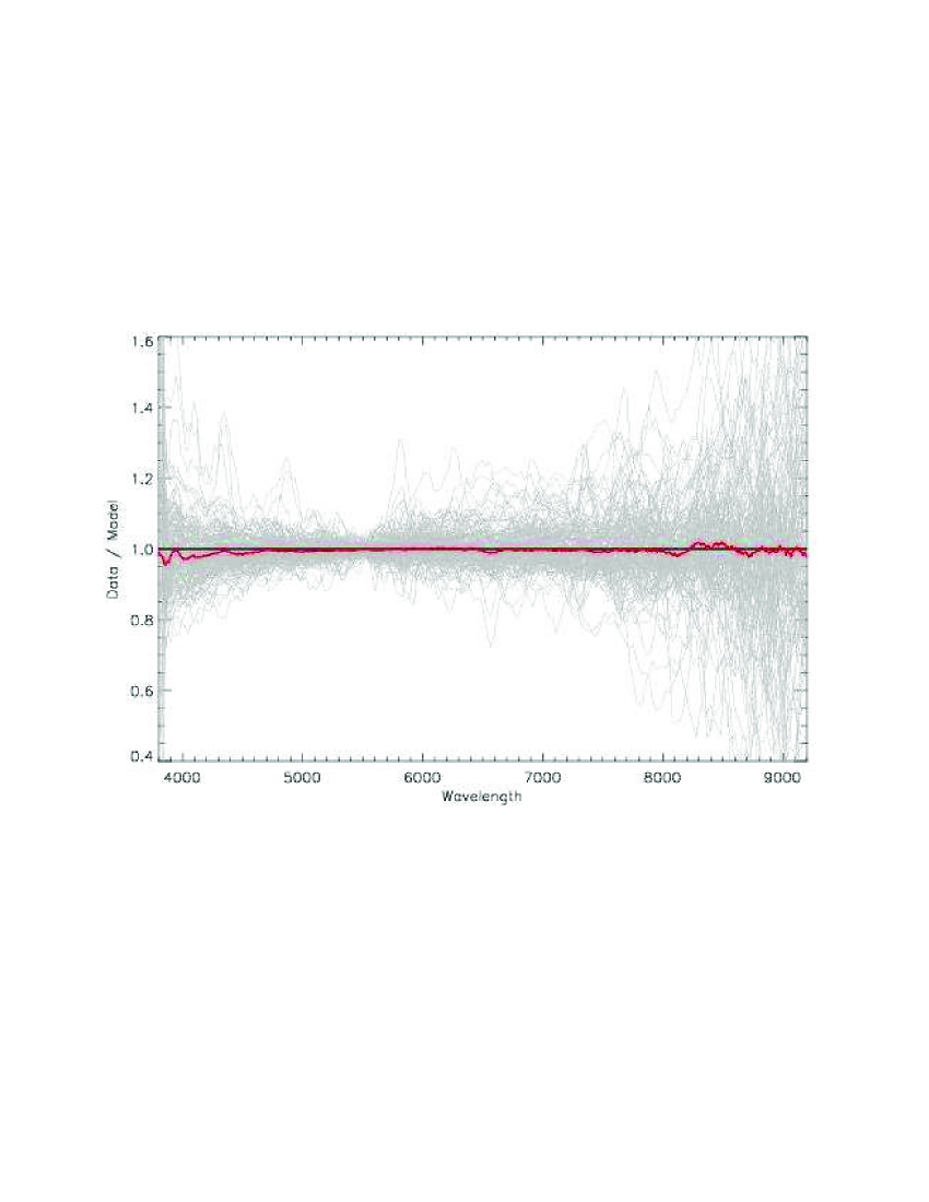
Figure 1: A test of the quality of spectrophotometric calibration. Each thin curve shows a spectrum of a hot white dwarf (which were not used in calibration) divided by its best-fit model. The thick red curve is the median of these curves.

The SDSS stellar spectra are used for:

1. Calibration of observations

2. More accurate and robust source identification than that based on photometric data alone

3. Accurate stellar parameters estimation

4. Radial velocity for kinematic studies

3.1 Calibration of SDSS spectra

Stellar spectra are used for the calibration of all SDSS spectra. On each spectroscopic plate, 16 objects are targeted as spectroscopic standards. These objects are color-selected to be similar in spectral type to the SDSS primary standard BD+17 4708 (an F8 star). The spectrum of each standard star is spectrally typed by comparing with a grid of theoretical spectra generated from Kurucz model atmospheres using the spectral synthesis code SPECTRUM (Gray et al., 2001). The flux calibration vector is derived from the average ratio of each star and its best-fit model, separately for each of the 2 spectrographs, and after correcting for Galactic reddening. Since the red and blue halves of the spectra are imaged onto separate CCDs, separate red and blue flux calibration vectors are produced. The spectra from multiple exposures are then combined with bad pixel rejection and rebinned to a constant dispersion. The absolute calibration is obtained by tying the $r$-band fluxes of the standard star spectra to the fiber magnitudes output by the photometric pipeline (fiber magnitudes are corrected to a constant seeing of 2 arcsec, with accounting for the contribution of flux from overlapping objects in the fiber aperture).

To evaluate the quality of spectrophotometric calibration on scales of order 100Å, the calibrated spectra of a sample of 166 hot DA white dwarfs drawn from the SDSS DR1 White Dwarf Catalog (Kleinman et al., 2004) are compared to theoretical models (DA white dwarfs are useful for this comparison because they have simple hydrogen atmospheres that can be accurately modeled). Figure 1 shows the results of dividing each white dwarf spectrum by its best fit model. The median of the curves shows a net residual of order 2% at the bluest wavelengths.

Another test of the quality of spectrophotometric calibration is provided by the comparison of imaging magnitudes and those synthesized from spectra, for details see Vanden Berk et al. (2004) and Smolčić et al. (2006). With the latest reductions the two types of magnitudes agree with an rms of $\sim$0.05 mag.

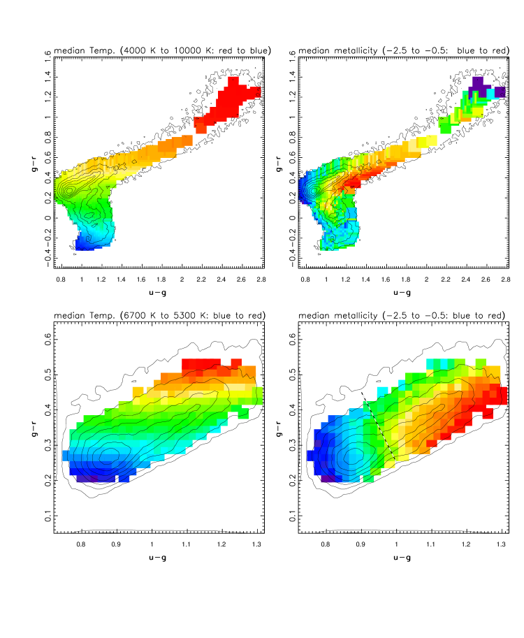
Figure 2: The top left panel shows the median effective temperature estimated from spectra of $\sim$40,000 stars as a function of the position in the $g-r$ vs. $u-g$ diagram based on imaging data. The temperature in each color-color bin is linearly color-coded from 4000 K (red) to 10,000 K (blue). The bottom left panel is analogous except that it shows the blue tip of the stellar locus with the effective temperature in the range 5300 K to 6700 K. The two right panels are analogous to the left panels, except that they show the median metallicity, linearly color-coded from -0.5 (red) to -2.5 (blue).

3.2 Source Identification

SDSS stellar spectra have been successfully used for confirmation of unresolved binary stars, low-metallicity stars, cold white dwarfs, L and T dwarfs, carbon stars, etc. For more details, we refer the reader to Adelman-McCarthy et al. (2006) and references therein.

3.3 Stellar Parameters Estimation

SDSS stellar spectra are of sufficient quality to provide robust and accurate stellar parameters such as effective temperature, gravity, metallicity, and detailed chemical composition. Here we study a correlation between the stellar parameters estimated by Beers et al. group (Allende Prieto et al., 2006) and the position of a star in the $g-r$ vs. $u-g$ color-color digram.

Figure 2 shows that the effective temperature determines the $g-r$ color, but has negligible impact on the $u-g$ color. The expression

$$\log(T_{\rm eff}/{\rm K})=3.877-0.26\,(g-r)$$ (1)

provides correct spectroscopic temperature with an rms of only 2% (i.e. about 100-200 K) for the $-0.3<g-r<1.0$ color range. While the median metallicity shows a more complex behavior as function of the $u-g$ and $g-r$ colors, it can still be utilized to derive photometric metallicity estimate. For example, for stars at the blue tip of the stellar locus ($u-g<1$), the expression

$$[Z/Z_{\odot}]=5.11\,(u-g)-6.33$$ (2)

reproduces the spectroscopic metallicity with an rms of only 0.3 dex.

These encouraging results are important for studies based on photometric data alone, and also demonstrate the robustness of parameters estimated from spectroscopic data.

3.4 Metallicity Distribution and Kinematics

Due to large sample size and faint limiting magnitude ($g\sim 20$), the SDSS stellar spectra are an excellent resource for studying the Milky Way metallicity distribution, kinematics and their correlation all the way to the boundary between the disk and halo at several kpc above the Galactic plane (Jurić et al., 2006). Here we present some preliminary results that illustrate the ongoing studies.

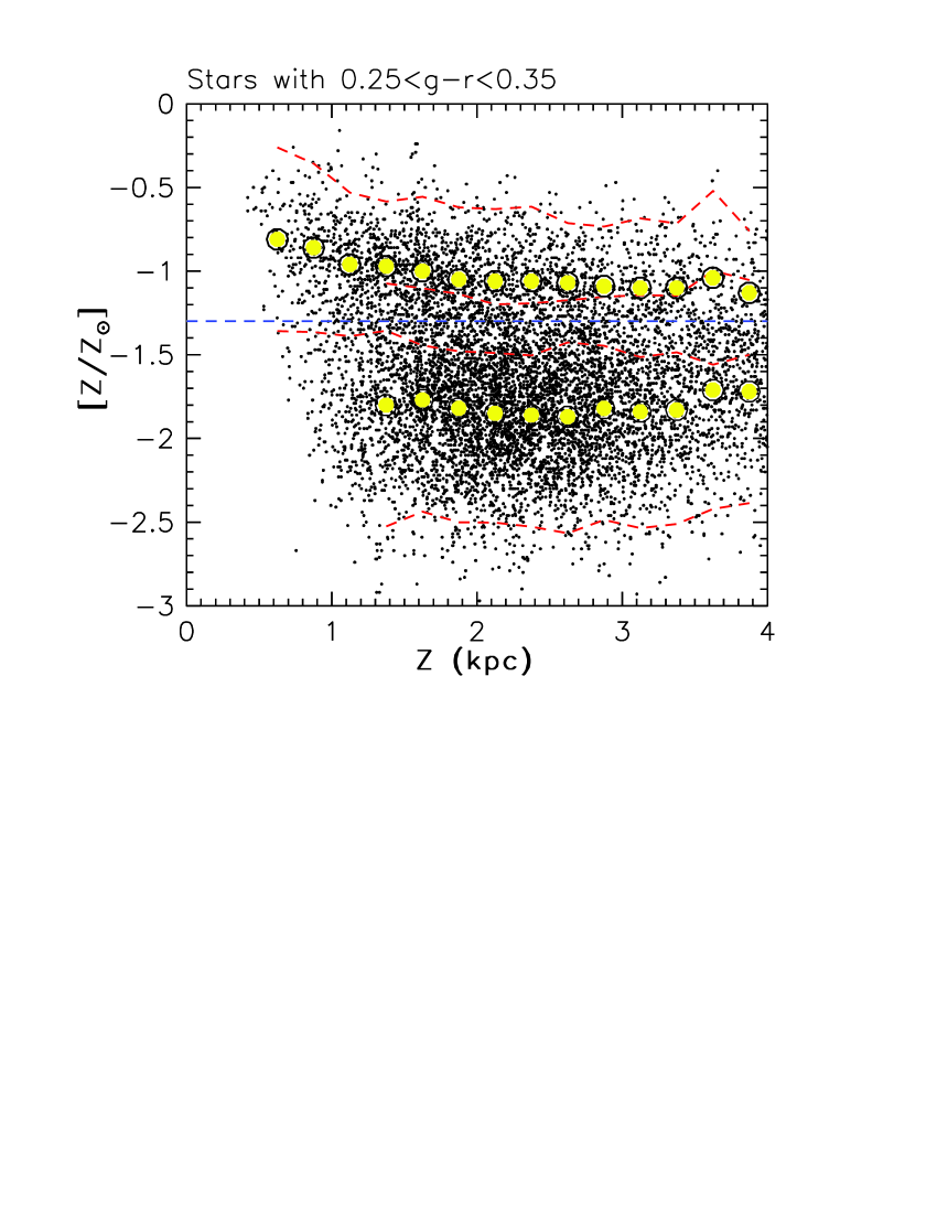
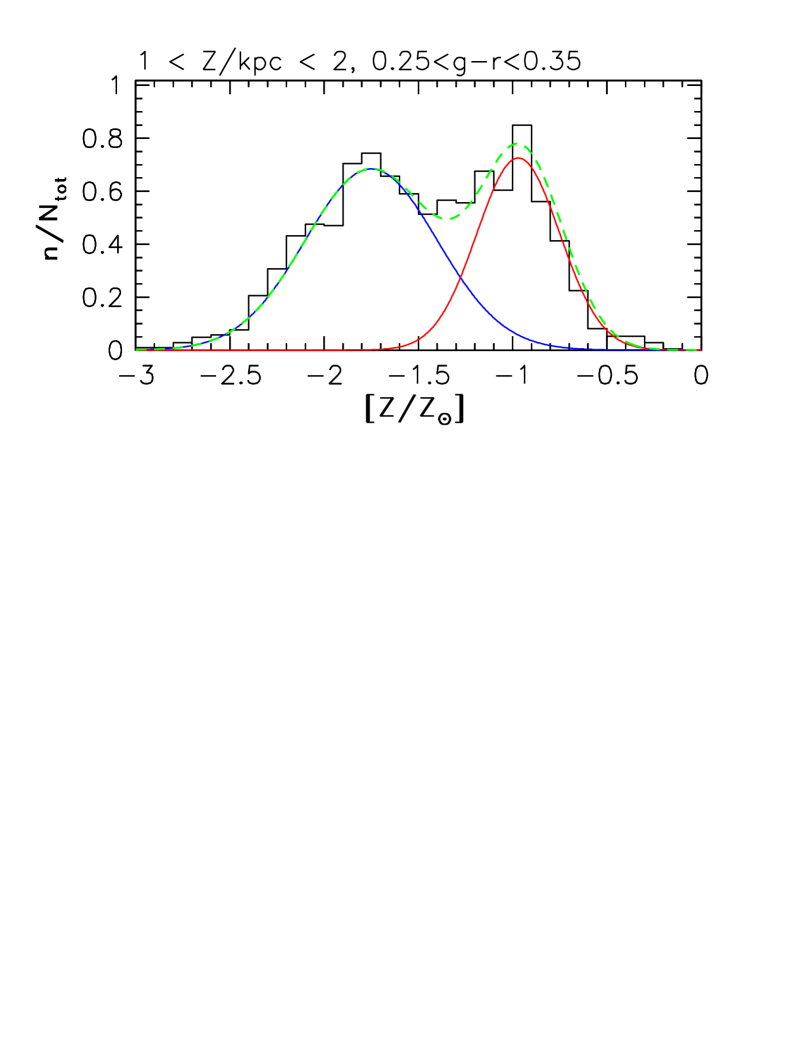
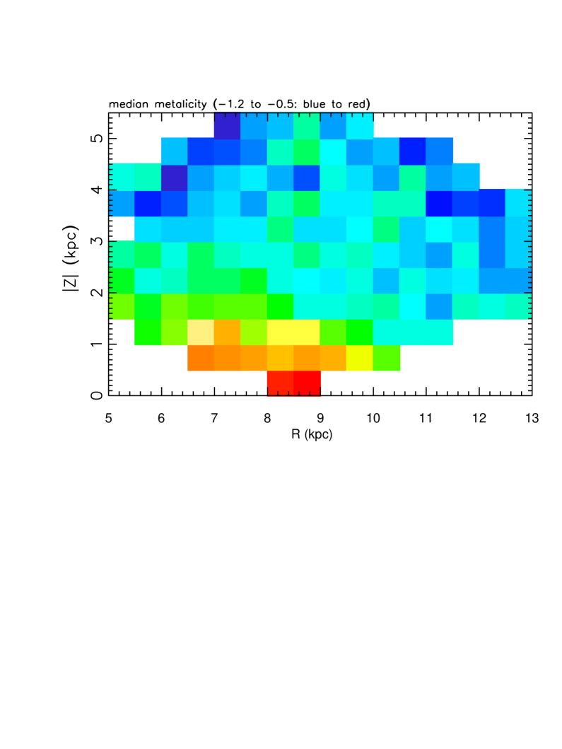
Figure 3: The dots in the top panel show the metallicity of stars with $0.25<g-r<0.35$ as a function of the height above the Galactic plane. The large symbols are the medians evaluated separately for the low-metallicity ($[Z/Z_{\odot}]<-1.3$) and high-metallicity ($[Z/Z_{\odot}]>-1.3$) subsamples, and the dashed lines show the 2$\sigma$ envelopes around the median. The histogram in the middle panel illustrates the bimodality of metallicity distribution for stars with heights above the galactic plane between 1 kpc and 2 kpc. The two solid lines are the best-fit Gaussians, and the dashed line is their sum. The dependence of the median metallicity for the high-metallicity subsample on the cylindrical galactic coordinates $R$ and $z$ is shown in the bottom panel (linearly color-coded from $-$1.2 to $-$0.5, blue to red). Note that the $z$ gradient is much larger than the $R$ gradient. For the low-metallicity subsample, these gradients are negligible.

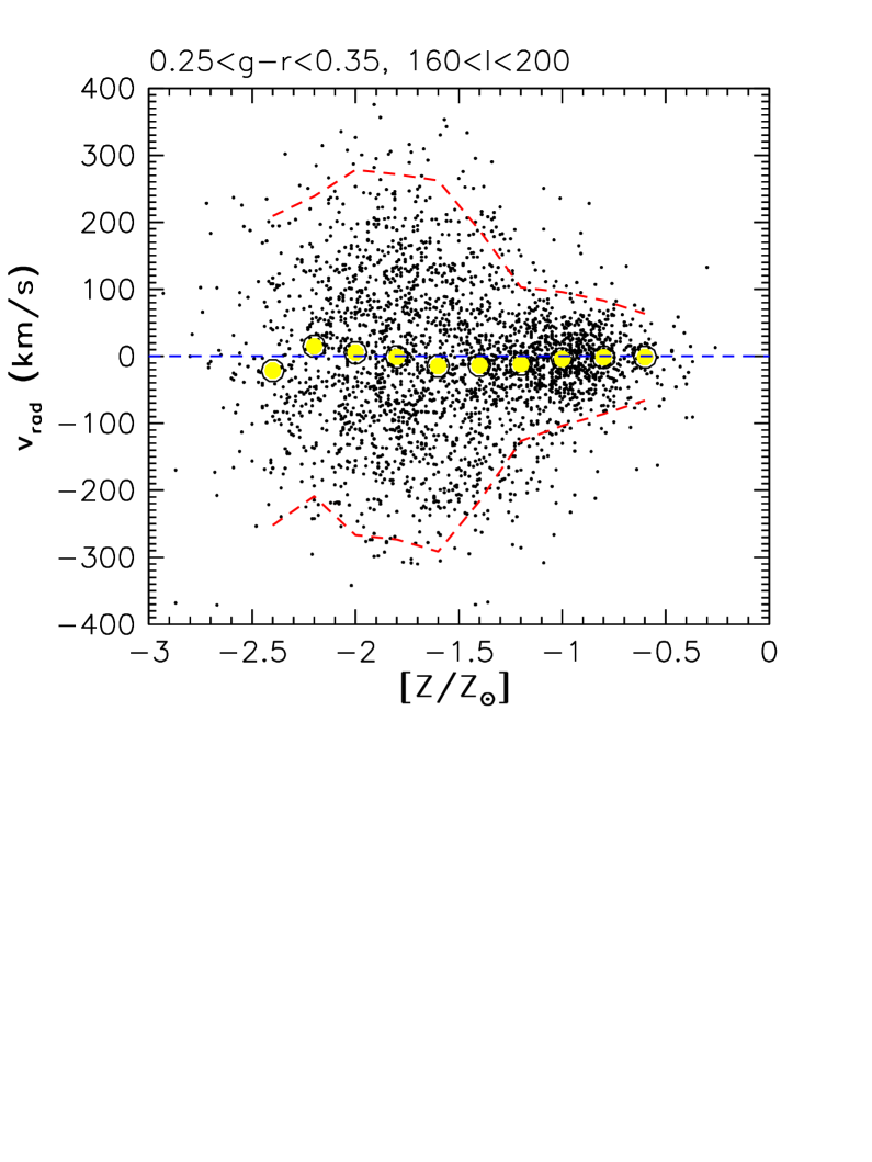
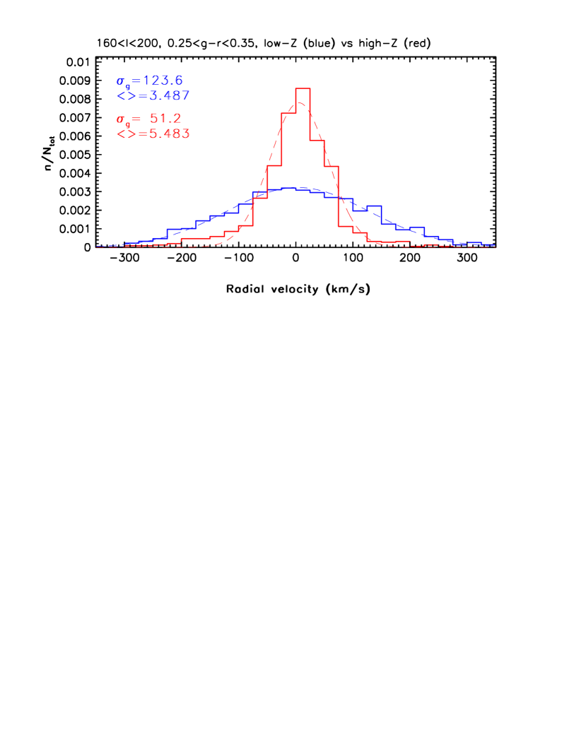
Figure 4: The dots in the top panel show the radial velocity as a function of metallicity for stars with $0.25<g-r<0.35$ and 160 $<l<$ 200 (towards anticenter, where the radial velocity corresponds to the $v_{R}$ velocity component). The large symbols are the medians evaluated in narrow metallicity bins, and the dashed lines show the 2$\sigma$ envelopes around the median. The radial velocity distributions for the low- and high-metallicity subsamples (separated by $[Z/Z_{\odot}]=-1.3$) are shown in the bottom panel, together with the best-fit Gaussians (dashed lines) and their parameters. Note that the velocity dispersion is $\sim$2.5 times larger for the low-metallicity subsample.

x

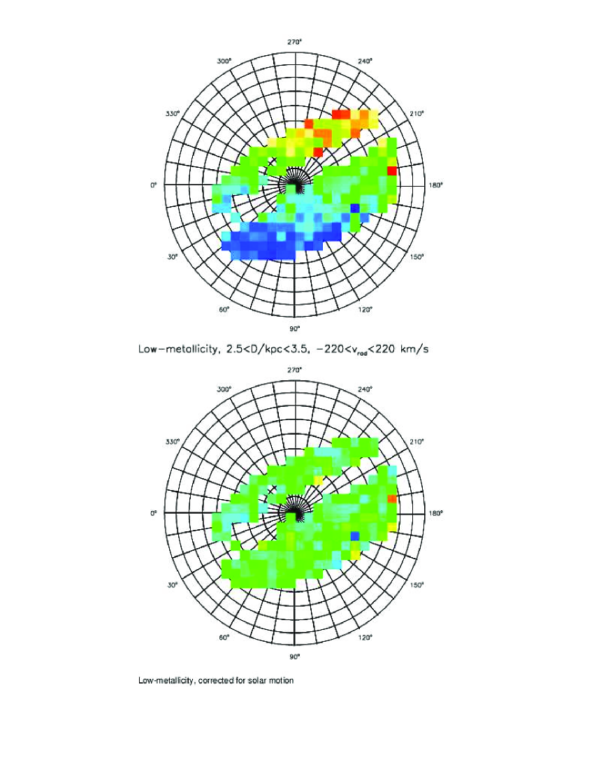
Figure 5: The top panel shows the median radial velocity in Lambert projection for stars from the low-metallicity $[Z/Z_{\odot}]<-1.3$ subsample, which have $b>0$ and are observed at distances between 2.5 kpc and 3.5 kpc. The radial velocity is linearly color-coded from -220 km/s to 220 km/s (blue to red, green corresponds to 0 km/s). The bottom panel is analogous, except that the radial velocity measurements are corrected for the canonical solar motion of 220 km/s towards ($l=90,b=0$).

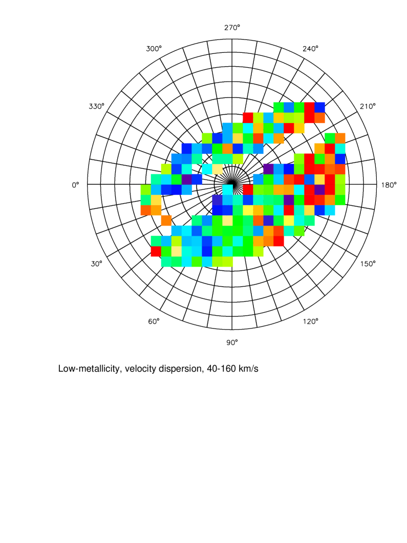
Figure 6: Analogous to Fig. 5, except that the velocity dispersion is shown (color-coded from 40 km/s to 160 km/s).

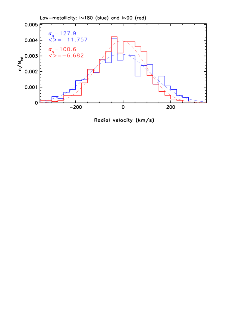
Figure 7: A comparison of the radial velocity distribution for low-metallicity stars observed towards $l\sim 90$ and $l\sim 180$. Note that the subsample observed towards the anti-center has a large velocity dispersion, in agreement with Figure 6.

3.4.1 The Bimodal Metallicity Distribution

In order to minimize various selection effects, we study a restricted sample of $\sim$10,000 blue main-sequence stars defined by $14.5<g<19.5$, $0.7<u-g<2.0$ and $0.25<g-r<0.35$. The last condition selects stars with the effective temperature in the narrow range 6000-6500 K. These stars are further confined to the main stellar locus by $|s|<0.04$, where the $s$ color, described by Ivezić et al. (2004), is perpendicular to the locus in the $g-r$ vs. $u-g$ color-color diagram (c.f. Fig. 2). We estimate distances using a photometric parallax relation derived by Jurić et al. (2006).

The metallicity distribution for stars from this sample that are at a few kpc from the galactic plane is clearly bimodal (see the middle panel in Fig. 3), with a local minimum at $[Z/Z_{\odot}]\sim-1.3$. Motivated by this bimodality, we split the sample into low- (L) and high-metallicity (H) subsamples and analyze the spatial variation of their median metallicity. As shown in the bottom panel in Fig. 3, the median metallicity of the H sample has a much larger gradient in the $z$ direction (distance from the plane), than in the $R$ direction (cylindrical galactocentric radius). In contrast, the median metallicity of the L sample shows negligible variation with the position in the Galaxy ($<$0.1 dex within 4 kpc from the Sun) and the whole distribution appears Gaussian, with the width of 0.35 dex and centered on $[Z/Z_{\odot}]=-1.75$.

The decrease of the median metallicity with $z$ for the H sample is well described by $[Z/Z_{\odot}]=-0.65-0.15\,Z/{\rm kpc}$ for $Z<1.5$ kpc and $[Z/Z_{\odot}]=-0.80-0.05\,Z/{\rm kpc}$ for $1.5<Z<4$ kpc (see the top panel in Fig. 3). For $Z<1$ kpc, most stars have $[Z/Z_{\odot}]>-1.3$ and presumably belong to thin and thick disks (for a recent determination of the stellar number density based on SDSS data that finds two exponential disks, see Jurić 2006). The decrease of the median metallicity with $z$ for the H sample could thus be interpreted as due to the increasing fraction of the lower-metallicity thick disk stars. However, it is puzzling that we are unable to detect any hint of the two populations. An analogous absence of a clear distinction between the thin and thick disks is also found when analyzing the radial velocity distribution.

3.4.2 The Metallicity–Kinematics Correlation

In addition to the bimodal metallicity distribution, the existence of two populations is also supported by the radial velocity distribution. As illustrated in Fig. 4, the low-metallicity component has about 2.5 times larger velocity dispersion than the high-metallicity component. Of course, this metallicity–kinematics correlation was known since the seminal paper by Eggen, Lynden-Bell & Sandage (1962), but here it is reproduced using a $\sim$100 times larger sample that probes a significantly larger Galaxy volume.

3.4.3 The Global Behavior of Kinematics

The large sample size enables a robust search for anomalous features in the global behavior of kinematics, e.g. Sirko et al. (2004). For example, while the variation of the median radial velocity for the low-metallicity subsample is well described by the canonical solar motion (Fig. 5), we find an isolated $\sim$1000 deg² large region on the sky where the velocity dispersion is larger (130 km/s) than for the rest of the sky (100 km/s), see Figs. 6 and 7. This is probably not a data artefact because the dispersion for the high-metallicity subsample does not show this effect. Furthermore, an analysis of the proper motion database constructed by Munn et al. (2004) finds that the same stars also have anomalous (non-zero) rotational velocity in the same sky region (Bond et al., 2006). This kinematic behavior could be due to the preponderance of stellar streams in this region (towards the anti-center, at high galactic latitudes, and at distances of several kpc). Bond et al. (2006) also find, using a sample of SDSS stars for which all three velocity components are known, that the halo (low-metallicity sample) does not rotate (at the $\sim$10 km/s level), while the rotational velocity of the high-metallicity sample decreases with the height above the galactic plane.

4 Conclusions

We show that stellar parameter estimates by Beers et al. show a good correlation with the position of a star in the $g-r$ vs. $u-g$ color-color diagram, thereby demonstrating their robustness as well as a potential for photometric stellar parameter estimation methods. We find that the metallicity distribution of the Milky Way stars at a few kpc from the galactic plane is clearly bimodal with a local minimum at $[Z/Z_{\odot}]\sim-1.3$. The median metallicity for the low-metallicity $[Z/Z_{\odot}]<-1.3$ subsample is nearly independent of Galactic cylindrical coordinates $R$ and $z$, while it decreases with $z$ for the high-metallicity $[Z/Z_{\odot}]>-1.3$ sample. We also find that the low-metallicity sample has $\sim$2.5 times larger velocity dispersion.

The samples discussed here are sufficiently large to constrain the global kinematic behavior and search for anomalies. For example, we find that low-metallicity stars observed at high galactic latitudes at distances of a few kpc towards Galactic anticenter have anomalously large velocity dispersion and a non-zero rotational component in a well-defined $\sim$1000 deg² large region, perhaps due to stellar streams.

These preliminary results are only brief illustrations of the great potential of the SDSS stellar spectroscopic database. This dataset will remain a cutting edge resource for a long time because other major ongoing and upcoming stellar spectroscopic surveys are either shallower (e.g. RAVE), or have a significantly narrower wavelength coverage (GAIA).