A Comparison of SDSS Standard Star Catalog for Stripe 82 with Stetson’s Photometric Standards

Abstract

We compare Stetson’s photometric standards with measurements listed in a standard star catalog constructed using repeated SDSS imaging observations. The SDSS catalog includes over 700,000 candidate standard stars from the equatorial stripe 82 ($|$Dec$|<$ 1.266 deg) in the RA range 20h 34’ to 4h 00’, and with the $r$ band magnitudes in the range 14–21. The distributions of measurements for individual sources demonstrate that the SDSS photometric pipeline correctly estimates random photometric errors, which are below 0.01 mag for stars brighter than (19.5, 20.5, 20.5, 20, 18.5) in ugriz, respectively (about twice as good as for individual SDSS runs). We derive mean photometric transformations between the SDSS gri and the BVRI system using 1165 Stetson stars found in the equatorial stripe 82, and then study the spatial variation of the difference in zeropoints between the two catalogs. Using third order polynomials to describe the color terms, we find that photometric measurements for main-sequence stars can be transformed between the two systems with systematic errors smaller than a few millimagnitudes. The spatial variation of photometric zeropoints in the two catalogs typically does not exceed 0.01 magnitude. Consequently, the SDSS Standard Star Catalog for Stripe 82 can be used to calibrate new data in both the SDSS ugriz and the BVRI systems with a similar accuracy.

¹ Department of Astronomy, University of Washington, Seattle, WA 98115, ² Department of Physics & Astronomy, Austin Peay State University, Clarksville, TN 37044, ³ Fermi National Accelerator Laboratory, P.O. Box 500, Batavia, IL 60510, ⁴ Princeton University Observatory, Princeton, NJ 08544, ⁵ New Mexico State University, Box 30001, 1320 Frenger St., Las Cruces, NM 88003 ⁶ Lawrence Berkeley National Laboratory, MS 50R5032, Berkeley, CA, 94720, ⁷ Department of Astronomy, Harvard University, 60 Garden St., Cambridge, MA 02138 ⁸ University of California–Santa Cruz, 1156 High St., Santa Cruz, CA 95060, ⁹ School of Physics and Astronomy, University of Southampton, Highfield, Southampton, SO17 1BJ, UK, ¹⁰ U.S. Naval Observatory, Flagstaff Station, P.O. Box 1149, Flagstaff, AZ 86002, ¹¹ Department of Astronomy, Case Western Reserve University, Cleveland, Ohio 44106 ¹² Apache Point Observatory, 2001 Apache Point Road, P.O. Box 59, Sunspot, NM 88349-0059 ¹³ University of Chicago, Astronomy & Astrophysics Center, 5640 S. Ellis Ave., Chicago, IL 60637

1. Introduction

Astronomical photometric data are usually calibrated using sets of standard stars whose brightness is known from previous work. The most notable modern optical standard star catalogs are Landolt standards (Landolt 1992) and Stetson standards (Stetson 2000, 2005). Both are reported on the Johnson-Kron-Cousins system (Landolt 1983 and references therein). The Landolt catalog provides magnitudes accurate to 1-2% in the $UBVRI$ bands for $\sim$500 stars in the $V$ magnitude range 11.5–16. Stetson has extended Landolt’s work to fainter magnitudes, and provided the community with $\sim$1-2% accurate magnitudes in the $BVRI$ bands for $\sim$15,000 stars in the magnitude range $V\mathrel{\hbox{\hbox to0.0pt{\hbox{\lower 4.0pt\hbox{$\sim$}}\hss}\hbox{$<$}}}20$. Most stars from both sets are distributed along the Celestial Equator, which facilitates their use from both hemispheres.

The data obtained by the Sloan Digital Sky Survey (SDSS, York et al. 2000) can be used to extend the work by Landolt and Stetson to even fainter levels, and to increase the number of standard stars to almost a million. In addition, SDSS has designed its own photometric system ($ugriz$, Fukugita et al. 1996) which is now in use at a large number of observatories worldwide. This widespread use of the $ugriz$ photometric system motivates the construction of a large standard star catalog with $\sim$1% accuracy. As a part of its imaging survey, SDSS has obtained many scans in the so-called Stripe 82 region, defined by $|$Dec$|<$ 1.266 deg and RA approximately in the range 20h – 4h. These repeated observations can be averaged to produce more accurate photometry than the nominal 2% single-scan accuracy (Ivezić et al. 2004).

We briefly describe the construction and testing of a standard star catalog in §2, and discuss its comparison with Stetson’s photometric standards in §3.

2. The SDSS standard star catalog for stripe 82

2.1. Overview of SDSS imaging data

SDSS is using a dedicated 2.5m telescope (Gunn et al. 2006) to provide homogeneous and deep ($r<22.5$) photometry in five pass-bands (Fukugita et al. 1996; Gunn et al. 1998; Smith et al. 2002; Hogg et al. 2002) repeatable to 0.02 mag (root-mean-square scatter, hereafter rms, for sources not limited by photon statistics, Ivezić et al. 2003) and with a zeropoint uncertainty of $\sim$0.02-0.03 (Ivezić et al. 2004). The survey sky coverage of close to $\sim$10,000 deg² in the Northern Galactic Cap, and $\sim$300 deg² in the Southern Galactic Hemisphere, will result in photometric measurements for well over 100 million stars and a similar number of galaxies. Astrometric positions are accurate to better than 0.1 arcsec per coordinate (rms) for sources with $r<20.5^{m}$ (Pier et al. 2003), and the morphological information from the images allows reliable star-galaxy separation to $r\sim$ 21.5^m (Lupton et al. 2001, 2003, Scranton et al. 2002).

Data from the imaging camera (thirty photometric, twelve astrometric, and two focus CCDs, Gunn et al. 1998) are collected in drift scan mode. The images that correspond to the same sky location in each of the five photometric bandpasses (these five images are collected over $\sim$5 minutes, with 54 sec for each exposure) are grouped together for processing as a field. A field is defined as a 36 seconds (1361 pixels, or 9 arcmin) long and 2048 pixels wide (13 arcmin) stretch of drift-scanning data from a single column of CCDs (sometimes called a scanline, for more details please see Stoughton et al. 2002, Abazajian et al. 2003, 2004, 2005, Adelman-McCarthy et al. 2006). Each of the six scanlines (called together a strip) is 13 arcmin wide. The twelve interleaved scanlines (or two strips) are called a stripe ($\sim$2.5 deg wide).

2.2. The photometric calibration of SDSS imaging data

SDSS 2.5m imaging data are photometrically calibrated using a network of calibration stars obtained in 1520 41.5$\times$41.5 arcmin² transfer fields, called secondary patches. These patches are positioned throughout the survey area and are calibrated using a primary standard star network of 158 stars distributed around the Northern sky (Smith et al. 2002). The primary standard star network is tied to an absolute flux system by the single F0 subdwarf star BD+17^∘4708, whose absolute fluxes in SDSS filters are taken from Fukugita et al. (1996). The secondary patches are grouped into sets of four, and are observed by the Photometric Telescope (hereafter PT) in parallel with observations of the primary standards. A set of four spans all 12 scanlines of a survey stripe along the width of the stripe, and the sets are spaced along the length of a stripe at roughly 15 degree intervals, which corresponds to an hour of scanning at the sidereal rate.

SDSS 2.5m magnitudes are reported on the ”natural system” of the 2.5m telescope defined by the photon-weighted effective wavelengths of each combination of SDSS filter, CCD response, telescope transmission, and atmospheric transmission at a reference airmass of 1.3 as measured at APO. The magnitudes are referred to as the $ugriz$ system (which is different from the “primed” system, $u^{\prime}g^{\prime}r^{\prime}i^{\prime}z^{\prime}$, that is defined by the PT). The reported magnitudes are corrected for the atmospheric extinction (using simultaneous observations of standard stars by the PT) and thus correspond to measurements at the top of the atmosphere (except for the fact that the atmosphere has an impact on the wavelength dependence of the photometric system response). The magnitudes are reported on the AB system (Oke & Gunn 1983) defined such that an object with a specific flux of $F_{\nu}$=3631 Jy has $m=0$ (i.e. an object with $F_{\nu}$=const. has an AB magnitude equal to the Johnson $V$ magnitude at all wavelengths). In summary, given a specific flux of an object at the top of the atmosphere, $F_{\nu}(\lambda)$, the reported SDSS 2.5m magnitude in a given band corresponds to (modulo random and systematic errors, which will be discussed later)

$$m=-2.5\log_{10}\left({F_{o}\over 3631\,{\rm Jy}}\right),$$ (1)

where

$$F_{o}=\int{F_{\nu}(\lambda)\phi(\lambda)d\lambda}.$$ (2)

Here, $\phi(\lambda)$ is the normalized system response for the given band,

$$\phi(\lambda)={\lambda^{-1}S(\lambda)\over\int{\lambda^{-1}S(\lambda)d\lambda}},$$ (3)

with the overall atmosphere+system throughput, $S(\lambda)$, available from the website given above (for a figure showing $\phi(\lambda)$ for the $ugriz$ system see Smolčić et al. 2006).

The quality of SDSS photometry stands out among available large-area optical sky surveys (Ivezić et al. 2003, 2004; Sesar et al. 2006). Nevertheless, the achieved accuracy is occasionally worse than the nominal 0.02-0.03 mag (root-mean-square scatter for sources not limited by photon statistics). Typical causes of substandard photometry include an incorrectly modeled PSF (usually due to fast variations of atmospheric seeing, or lack of a sufficient number of the isolated bright stars needed for modeling the PSF), unrecognized changes in atmospheric transparency, errors in photometric zeropoint calibration, effects of crowded fields at low Galactic latitudes, an undersampled PSF in excellent seeing conditions ($\mathrel{\hbox{\hbox to0.0pt{\hbox{\lower 4.0pt\hbox{$\sim$}}\hss}\hbox{$<$}}}0.8$ arcsec; the pixel size is 0.4 arcsec), incorrect flatfield, or bias vectors, scattered light correction, etc. Such effects can conspire to increase the photometric errors to levels as high as 0.05 mag (with a frequency, at that error level, of roughly one field per thousand). However, when multiple scans of the same sky region are available, many of these errors can be minimized by properly averaging photometric measurements.

2.3. The catalog construction and internal tests

A detailed description of the catalog construction, including the flatfield corrections, and various tests of its photometric quality can be found in Ivezić et al. (2006). Here we only briefly describe the main catalog properties.

The catalog is based on 58 SDSS runs from stripe 82 (approximately 20h $<$ RA $<$ 04h and $|$Dec$|<$ 1.266) obtained in mostly photometric conditions (as indicated by the calibration residuals, infrared cloud camera, and tests performed by runQA quality assessment pipeline). Candidate standard stars from each run are selected by requiring

1. that objects are unresolved (classified as STAR by the photometric pipeline)

2. that they have quoted photometric errors (as computed by the photometric pipeline) smaller than 0.05 mag in at least one band, and

3. that processing flags BRIGHT, SATUR, BLENDED, EDGE are not set.

These requirements select unsaturated sources with sufficiently high signal-to-noise per single observation to approach the final photometric errors of 0.02 mag or smaller.

After positionally matching (within 1 arcsec) all detections of a single star, various photometric statistics such as mean, median, root-mean-square scatter, number of observations, and $\chi^{2}$ per degree of freedom ($\chi^{2}_{pdf}$) are computed in each band. This initial catalog of multi-epoch observations includes 924,266 stars with at least 4 observations in each of the $g$, $r$ and $i$ bands. The median number of observations per star and band is 10, and the total number of photometric measurements is $\sim$40 million. The errors for the averaged photometry are below 0.01 mag at the bright end. These errors are reliably computed by photometric pipeline, as indicated by the $\chi^{2}_{pdf}$ distributions.

Adopted candidate standard stars must have at least 4 observations in each of the $g$, $r$ and $i$ bands and, to avoid variable sources, $\chi^{2}_{pdf}$ less than 3 in the $gri$ bands. The latter cut rejects about 20% of stars. We also limit the RA range to 20h 34’ $<$ RA $<$ 04h 00’, which provides a simple areal definition (together with $|$Dec$|<$1.266 deg) while excluding only a negligible fraction of stars. These requirements result in a catalog with 681,262 candidate standard stars. Of those, 638,671 have the random error for the median magnitude in the $r$ band smaller than 0.01 mag, and 131,014 stars have the random error for the median magnitude smaller than 0.01 mag in all five bands.

The internal photometric consistency of this catalog is tested using a variety of methods, including the position of the stellar locus in the multi-dimensional color space, color-redshift relations for luminous red galaxies, and a direct comparison with the secondary standard star network. While none of this methods is without its disadvantages, together they suggest that the internal photometric zeropoints are spatially stable at the 1% level.

3. An external test of catalog quality based on Stetson’s standards

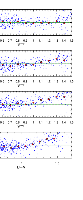
Figure 1.: An illustration of the need for non-linear color terms when transforming SDSS photometry to the BVRI system. The small dots in the top panel show the residuals (in magnitudes) for the cubic $B-g$ transformation based on eq. 4, as a function of the $g-r$ color. The large symbols show the medians for 0.1 mag wide $g-r$ bins. The second panel is analogous to the top panel, except that a best-fit linear transformation is used ($B-g=0.345\,(g-r)+0.205$). Note the increased deviation of median residuals from zero. The third panel shows residuals for the relation $B-V=0.949\,(g-r)+0.197$ and demonstrates that even such a color vs. color relation is measurably non-linear. The bottom panel shows that this is not a peculiarity of the $g-$ color because a transformation based on the $B-V$ color, $B-g=0.364\,(B-V)+0.133$, is also measurably non-linear.

Table 1.: SDSS to BVRI transformations

color	$<>_{med}^{a}$	$\sigma_{med}^{b}$	$\chi_{med}^{c}$	$<>_{all}^{d}$	$\sigma_{all}^{e}$	A	B	C	Df
$B-g$	-1.6	8.7	1.4	1.0	32	0.2628	-0.7952	1.0544	0.0268
$V-g$	0.8	3.9	1.0	0.9	18	0.0688	-0.2056	-0.3838	-0.0534
$R-r$	-0.1	5.8	0.9	1.2	15	-0.0107	0.0050	-0.2689	-0.1540
$I-i$	0.9	6.1	1.0	1.2	19	-0.0307	0.1163	-0.3341	-0.3584

While the tests based on SDSS data suggest that the internal photometric zeropoints are spatially stable at the 1% level, it is of course prudent to verify this conclusion using an external independent dataset. The only large external dataset with sufficient overlap, depth and accuracy to test the quality of the Stripe 82 catalog is that provided by Stetson (2000, 2005). Stetson’s catalog lists photometry in the $BVRI$ bands (Stetson’s photometry is tied to Landolt’s standards) for $\sim$1,200 stars in common (most have $V<19.5$). We synthesize the $BVRI$ photometry from SDSS $gri$ measurements using photometric transformations of the following form

$$m_{\rm Stetson}-\mu_{\rm SDSS}=A\,c^{3}+B\,c^{2}+C\,c+D,$$ (4)

where $m=(BVRI)$ and $\mu=(g,g,r,i)$, respectively, and the color $c$ is measured by SDSS ($g-r$ for the $B$ and $V$ transformations, and $r-i$ for the $R$ and $I$ transformations). The measurements are not corrected for the ISM reddening. Traditionally, such transformations are assumed to be linear in color We use higher-order terms in eq. 4 because at the 1-2% level there are easily detectable deviations from linearity for all color choices, as shown in Fig. 1. The best-fit coefficients for the transformation of SDSS $gri$ measurements to the $BVRI$ system are listed in Table 1, as well as low-order statistics for the $m_{\rm Stetson}-\mu_{\rm SDSS}$ difference distribution. We find no trends as a function of magnitude at the $<0.005$ mag level.

We have also tested for the effects of interstellar dust reddening and metallicity on the adopted photometric relations. For about half of stars in common, the SFD map (Schlegel, Finkbeiner & Davis 1998) lists $E(B-V)>0.15$. The differences in median residuals for these stars and those with smaller $E(B-V)$ (the median $E(B-V)$ are 0.31 and 0.04) are always less than 0.01 mag (the largest difference is 8 millimag for the $B-g$ transformation).

Stars at the blue tip of the stellar locus with $u-g<1$ are predominantly low-metallicity stars (Bond et al. 2006, in prep.), as illustrated in Fig. 2. Fig. 3 shows that the median residuals for $m_{\rm Stetson}-\mu_{\rm SDSS}$ are the same for the $0.8<u-g<0.95$ and $1.0<u-g<1.15$ subsamples to within their measurement errors ($\sim$10 millimag). There is a possibilty that the offset is somewhat larger for the $B-g$ transformation for stars with $u-g<0.9$, but its statistical significance is low. If this is a true effect, it implies a gradient with respect to metallicity of about 0.02 mag/dex.

We conclude that the SDSS catalog described here could also be used to calibrate the data to the BVRI system without a loss of accuracy due to transformations between the two systems.

Figure 2.: The median effective temperature and median metallicity estimated from SDSS spectra of $\sim$40,000 stars by Allende Prieto et al. (2006), shown as a function of the position in the $g-r$ vs. $u-g$ diagram based on SDSS imaging data. In the left panel, the temperature in each color-color bin is linearly color-coded from 5300 K (red) to 6,700 K (blue). The right panel is analogous, except that it shows the median metallicity, linearly color-coded from -0.5 (red) to -2.5 (blue).

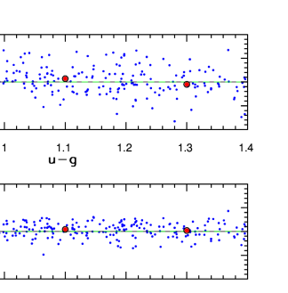
Figure 3.: An illustration of the effects of metallicity on photometric transformations. Here the $u-g$ color serves as a proxy for metallicity (see the right panel in Fig. 2). The panels shows the dependence of the $B-g$ residuals (top) and the $V-g$ residuals (bottom) on the $u-g$ color. The effects of metallicity on photometric transformations from the SDSS to the BVRI system appear smaller than about 0.01 mag, and possibly somewhat larger for the $B-g$ transformation for stars with $u-g<0.9$.

3.1. The spatial variations of the zeropoints

The $BVRI$ photometry from Stetson and that synthesized from SDSS agree at the level of 0.02 mag (rms scatter for the magnitude differences of individual stars; note that the systems are tied to each other to within a few millimags by transformations listed in Table 1). This scatter is consistent with the claimed accuracy of both catalogs (the magnitude differences normalized by the implied error bars are well described by Gaussians with widths in the range 0.7–0.8). This small scatter allows us to test for the spatial variation of zeropoints between the two datasets, despite the relatively small number of stars in common.

Stars in common are found in four isolated regions that coincide with historical and well-known Kapteyn Selected Areas 113, 92, 95, and 113. We determine the zeropoint offsets between the SDSS and Stetson’s photometry for each region separately by synthesizing $BVRI$ magnitudes from SDSS $gri$ photometry, and comparing them to Stetson’s measurements. The implied zeropoint errors (which, of course, can be due to either SDSS or Stetson’s dataset, or both) are listed in Table 2. For regions 1-3 the implied errors are only a few millimags (except for the $B-g$ color in region 1). The discrepancies are much larger for the three red colors in region 4. A comparison with the results of internal SDSS tests described by Ivezić et al. (2006) suggests that these discrepancies are more likely due to zeropoint offsets in Stetson’s photometry for this particular region, than to problems with SDSS photometry. We contacted P. Stetson who confirmed that his observing logs were consistent with this conclusion. Only a small fraction of stars from Stetson’s list are found in this region.

Given the results presented in this Section, we conclude that the rms for the spatial variation of zeropoints in the SDSS Stripe 82 catalog is below 0.01 mag in the $gri$ bands.

Table 2.: Photometric zeropoint spatial variations

color	$x_{R1}^{a}$	$\sigma_{R1}^{b}$	N${}_{R1}^{c}$	$x_{R2}^{a}$	$\sigma_{R2}^{b}$	N${}_{R2}^{c}$	$x_{R3}^{a}$	$\sigma_{R3}^{b}$	N${}_{R3}^{c}$	$x_{R4}^{a}$	$\sigma_{R4}^{b}$	N${}_{R4}^{c}$
$B-g$	$-$29	21	92	6	27	165	8	42	155	$-$4	27	281
$V-g$	0	17	99	0	15	217	6	25	161	17	19	282
$R-r$	$-$6	16	58	4	16	135	$-$8	12	11	39	27	60
$I-i$	$-$11	16	94	6	18	205	2	16	124	19	15	47

4. Discussion and Conclusions

Using repeated SDSS measurements, we have constructed a catalog of about 700,000 candidate standard stars. Several independent tests suggest that both random photometric errors and internal systematic errors in photometric zeropoints are below 0.01 mag (about 2-3 times as good as individual SDSS runs) for stars brighter than (19.5, 20.5, 20.5, 20, 18.5) in ugriz, respectively. This is by far the largest existing catalog with multi-band optical photometry accurate to $\sim$1%. The catalog is publicly available from the SDSS Web Site.

In this contribution, we have tested the photometric quality of this catalog by comparing it to Stetson’s standard stars. Using third order polynomials to describe the color terms between the SDSS and BVRI systems, we find that photometric measurements for main-sequence stars can be transformed between the two systems with systematic errors smaller than a few millimagnitudes. The spatial variation of photometric zeropoints in the two catalogs typically does not exceed 0.01 magnitude. Consequently, the SDSS Standard Star Catalog for Stripe 82 can be used to calibrate new data in both the SDSS ugriz and the BVRI systems with a similar accuracy.

Acknowledgments.

Funding for the SDSS and SDSS-II has been provided by the Alfred P. Sloan Foundation, the Participating Institutions, the National Science Foundation, the U.S. Department of Energy, the National Aeronautics and Space Administration, the Japanese Monbukagakusho, the Max Planck Society, and the Higher Education Funding Council for England. The SDSS Web Site is http://www.sdss.org/.

The SDSS is managed by the Astrophysical Research Consortium for the Participating Institutions. The Participating Institutions are the American Museum of Natural History, Astrophysical Institute Potsdam, University of Basel, Cambridge University, Case Western Reserve University, University of Chicago, Drexel University, Fermilab, the Institute for Advanced Study, the Japan Participation Group, Johns Hopkins University, the Joint Institute for Nuclear Astrophysics, the Kavli Institute for Particle Astrophysics and Cosmology, the Korean Scientist Group, the Chinese Academy of Sciences (LAMOST), Los Alamos National Laboratory, the Max-Planck-Institute for Astronomy (MPIA), the Max-Planck-Institute for Astrophysics (MPA), New Mexico State University, Ohio State University, University of Pittsburgh, University of Portsmouth, Princeton University, the United States Naval Observatory, and the University of Washington.

References

- (1) Abazajian, K., Adelman, J.K., Agueros, M., et al. 2003, AJ, 126, 2081
- (2) Abazajian, K., Adelman, J.K., Agueros, M., et al. 2004, AJ, 128, 502
- (3) Abazajian, K., Adelman-McCarthy, J.K., Agüeros, M., et al. 2005, AJ, 129, 1755
- Adelman-McCarthy et al. (2006) Adelman-McCarthy, J.K., et al. 2006, ApJS, 162, 38
- Allende Prieto et al. (2006) Allende Prieto, C., Beers, T.C., Wilhelm, R. et al. 2006, ApJ, 636, 804
- (6) Fukugita, M., Ichikawa, T., Gunn, J.E., Doi, M., Shimasaku, K., & Schneider, D.P. 1996, AJ, 111, 1748
- Gunn et al. (1998) Gunn, J.E., Carr, M., Rockosi, C., et al. 1998, AJ, 116, 3040
- Gunn et al. (2006) Gunn, J.E., Siegmund, W.A., Mannery, E.J., et al. 2006, AJ, 131, 2332
- (9) Hogg, D.W., Finkbeiner, D.P., Schlegel, D.J. & Gunn, J.E. 2002, AJ, 122, 2129
- Ivezić et al. (2003) Ivezić, Ž., Lupton, R.H., Anderson, S., et al. 2003, Proceedings of the Workshop Variability with Wide Field Imagers, Mem. Soc. Ast. It., 74, 978 (also astro-ph/0301400)
- Ivezić et al. (2004) Ivezić, Ž., Lupton, R.H., Schlegel, D.J. et al. 2004, AN, 325, 583
- Ivezić et al. (2006) Ivezić, Ž., Smith, J.A., Miknaitis, G. et al. 2006, submitted to AJ
- (13) Landolt, A.U. 1983, AJ, 88, 439
- (14) Landolt, A.U. 1992, AJ, 104, 340
- Lupton, Gunn & Szalay (1999) Lupton, R.H., Gunn, J.E., & Szalay, A. 1999, AJ, 118, 1406
- Lupton et al. (2001) Lupton, R.H., Gunn, J.E., Ivezić, Ž., Knapp, G.R., Kent, S. & Yasuda, N. 2001, in ASP Conf. Ser. 238, Astronomical Data Analysis Software and Systems X, eds. F. R. Harnden, Jr., F. A. Primini, and H. E. Payne (San Francisco: Astr. Soc. Pac.), p. 269 (also astro-ph/0101420)
- Lupton et al. (2003) Lupton, R.H., Ivezić, Ž., Gunn, J.E., Knapp, G.R., Strauss, M.A. & Yasuda, N. 2003, in “Survey and Other Telescope Technologies and Discoveries”, Tyson, J.A. & Wolff, S., eds. Proceedings of the SPIE, 4836, 350
- Oke & Gunn (1983) Oke, J.B., & Gunn, J.E. 1983, ApJ, 266, 713
- Pier et al. (2003) Pier, J.R., Munn, J.A., Hindsley, R.B., Hennesy, G.S., Kent, S.M., Lupton, R.H. & Ivezić, Ž. 2003, AJ, 125, 1559
- Schlegel, Finkbeiner & Davis (1998) Schlegel, D., Finkbeiner,D.P. & Davis, M. 1998, ApJ500, 525
- (21) Scranton, R., Johnston, D., Dodelson, S., et al. 2002, ApJ, 579, 48
- Sesar et al. (2006) Sesar, B., Svilković, D., Ivezić, Ž., et al. 2006, AJ, 131, 2801
- (23) Smith, J.A., Tucker, D.L., Kent, S.M., et al. 2002, AJ, 123, 2121
- (24) Smolčić, V., Ivezić, Ž., Gaćeša, M., et al. 2006, MNRAS, 371, 121
- (25) Stetson, P.B. 2000, PASP, 112, 925
- (26) Stetson, P.B. 2005, PASP, 117, 563
- Stoughton et al. (2002) Stoughton, C., Lupton, R.H., Bernardi, M., et al. 2002, AJ, 123, 485
- York et al. (2000) York, D.G., Adelman, J., Anderson, S., et al. 2000, AJ, 120, 1579