LECTURE NOTES ON THE FORMATION AND
EARLY EVOLUTION OF PLANETARY SYSTEMS111Astrophysics
of Planet Formation (Armitage, 2010) is a graduate level textbook based on earlier versions of these notes.
I plan to continue updating these notes as an open access resource.
Abstract
These notes provide an introduction to the theory of the formation and early evolution of planetary systems. Topics covered include the structure, evolution and dispersal of protoplanetary disks; the formation of planetesimals, terrestrial and gas giant planets; and orbital evolution due to gas disk migration, planetesimal scattering, planet-planet interactions, and tides.
I Introduction
The theoretical study of planet formation has a long history. Many of the fundamental ideas in the theory of terrestrial planet formation were laid out by Safronov (1969) in his monograph “Evolution of the Protoplanetary Cloud and Formation of the Earth and the Planets”. The core accretion theory for gas giant formation was discussed by Cameron in the early 1970’s (Perri & Cameron, 1973) and had been developed in recognizable detail by 1980 (Mizuno, 1980). The data that motivated and tested these theories, however, was relatively meagre and limited to the Solar System. The last twenty-five years have seen a wealth of new observations, including imaging and spectroscopy of protoplanetary disks, the discovery of the Solar System’s Kuiper Belt, and the detection and characterization of extrasolar planetary systems. Many of these observations have revealed unexpected properties of disks and planetary systems, highlighting not so much gaps in our theoretical knowledge as a lack of understanding of how known physical processes combine to form the planetary systems.
The goal of these notes is to introduce the concepts underlying planet formation, via a mix of worked-through derivations and (necessarily incomplete) references to the literature. The main questions we hope to answer are,
-
•
How small solid particles grown to macroscopic dimensions within the environment of protoplanetary disks.
-
•
How terrestrial and giant planets form.
-
•
What processes determine the final architecture of planetary systems, and might explain the astounding diversity of observed extrasolar planets.
First though, we briefly review observational properties of the Solar System and extrasolar planetary systems that we might hope a theory of planet formation would explain.
I.1 Critical Solar System observations
I.1.1 Architecture
| Mercury | 0.387 | 0.206 | 7.0∘ | ||
|---|---|---|---|---|---|
| Venus | 0.723 | 0.007 | 3.4∘ | ||
| Earth | 1.000 | 0.017 | 0.0∘ | ||
| Mars | 1.524 | 0.093 | 1.9∘ | ||
| Jupiter | 5.203 | 0.048 | 1.3∘ | ||
| Saturn | 9.537 | 0.054 | 2.5∘ | ||
| Uranus | 19.191 | 0.047 | 0.8∘ | ||
| Neptune | 30.069 | 0.009 | 1.8∘ |
The orbital properties, masses and radii of the Solar System’s planets are listed in Table I. The dominant planets in the Solar System are our two gas giants, Jupiter and Saturn. These planets are composed primarily of hydrogen and helium – like the Sun – though they have a higher abundance of heavier elements as compared to Solar composition. Saturn is known to have a substantial core. Descending in mass there are two ice giants (Uranus and Neptune) composed of water, ammonia, methane, silicates and metals, plus low mass hydrogen / helium atmospheres; two large terrestrial planets (Earth and Venus) plus two smaller terrestrial planets (Mercury and Mars). Apart from Mercury, all of the planets have low eccentricities and orbital inclinations. They orbit in a plane that is approximately, but not exactly, perpendicular to the Solar rotation axis (the misalignment angle is about ).
In the Solar System the giant and terrestrial planets are clearly segregated in orbital radius, with the inner zone occupied by the terrestrial planets being separated from the outer giant planet region by the main asteroid belt. The orbital radii of the giant planets coincide with where we expect the protoplanetary disk to have been cool enough for ices to have been present. This is a significant observation in the classical theory of giant planet formation, since in that theory the time scale for giant planet formation depends upon the mass of condensable materials. One would therefore expect faster growth to occur in the outer ice-rich part of the protoplanetary disk.
I.1.2 Mass and angular momentum
The mass of the Sun is , made up of hydrogen (fraction by mass ), helium () and “metals” (which includes everything else, ). One observes immediately that,
| (1) |
i.e. most of the heavy elements in the Solar System are found in the Sun rather than in the planets. If most of the mass in the Sun passed through a disk during star formation the planet formation process need not be very efficient.
The angular momentum budget for the Solar System is dominated by the orbital angular momentum of the planets. The angular momentum in the Solar rotation is,
| (2) |
assuming for simplicity solid body rotation. Taking and adopting (roughly appropriate for a star with a radiative core), . By comparison the orbital angular momentum of Jupiter is,
| (3) |
This result implies that substantial segregation of mass and angular momentum must have taken place during (and subsequent to) the star formation process. We will look into how such segregation arises during disk accretion later.
I.1.3 Minimum mass Solar Nebula
We can use the observed masses and compositions of the planets to derive a lower limit to the amount of gas that must have been present when the planets formed. This is called the Minimum Mass Solar Nebula Weidenschilling (1977). The procedure is:
-
1.
Start from the known mass of heavy elements (say iron) in each planet, and augment this mass with enough hydrogen and helium to bring the mixture to Solar composition. This is a mild augmentation for Jupiter, but a lot more for the Earth.
-
2.
Divide the Solar System into annuli, with one planet per annulus. Distribute the augmented mass for each planet uniformly across the annuli, to yield a characteristic gas surface density (units ) at the location of each planet.
The result is that between Venus and Neptune (and ignoring the asteroid belt) . The precise normalization is mostly a matter of convention, but if one needs a specific number the most common value used is that due to Hayashi (1981),
| (4) |
Integrating out to 30 AU the enclosed mass is around 0.01 , which is in the same ball park as estimates of protoplanetary disk masses observed around other stars.
As the name should remind you this is a minimum mass. It is not an estimate of the disk mass at the time the Sun formed, nor is the scaling necessarily the actual surface density profile for a protoplanetary disk. Theoretical models of disks based on the -prescription predict a shallower slope more akin to (Bell et al., 1997), while models based on first-principles calculations of disk angular momentum transport suggest a complex profile that is not well-described by a single power-law. Observations of protoplanetary disks around other stars do not directly probe the planet-forming region at a few AU, although on larger scales (beyond 20 AU) sub-mm images are consistent with a median profile (Andrews et al., 2009).
I.1.4 Resonances
A resonance occurs when there is a near-exact relation between characteristic frequencies of two bodies. For example, a mean-motion resonance between two planets with orbital periods and occurs when,
| (5) |
with , integers (the resonance is typically important if and , or their difference, are small integers). The “approximately equal to” sign in this expression reflects the fact that resonances have a finite width, which varies with the particular resonance and with the eccentricities of the bodies involved. Resonant widths can be calculated precisely, though the methods needed to do so are beyond the scope of these notes (a standard reference is Murray & Dermott, 1999). In the Solar System Neptune and Pluto (along with many other Kuiper Belt objects) are in a 3:2 resonance, while Jupiter and Saturn are close to but outside a 5:2 mean-motion resonance222A delightful account of how it was recognized that this proximity influences the motion of Jupiter and Saturn is in Lovett (1895).. There are many resonant pairs among planetary moons. Jupiter’s satellites Io, Europa and Ganymede, for example, form a resonant chain in which Io is in 2:1 resonance with Europa, which itself is in a 2:1 resonance with Ganymede. In the Saturnian system, the small moons Prometheus and Pandora occupy a 121:118 resonance. If planetary (or satellite) orbits were distributed randomly, subject only to the requirement that they be stable for long periods, then the chances that two bodies would find themselves in a resonance is low. Seeing a resonance is thus strong circumstantial evidence that dissipative processes (tides being the prototypical example) resulted in orbital evolution and trapping into resonance at some point in the past history of the system (Goldreich, 1965).
Although there are no mean-motion resonances today between the Solar System’s major planets, other resonances are dynamically important. In particular, secular resonances, which occur when the precession frequencies of two bodies match, couple the dynamics of the giant planets to that of the asteroid belt and inner Solar System. The resonance, for example, which roughly speaking corresponds to the precession rate of Saturn’s orbit, defines the inner edge of the asteroid belt. It is important for the delivery of meteorites and Near Earth Asteroids to the Earth (Scholl & Froeschle, 1991).
I.1.5 Minor bodies
As a rough generalization the Solar System is dynamically full, in that most locations where test particle orbits would be stable for 5 Gyr are, in fact, occupied by minor bodies (e.g., for the outer Solar System see Holman & Wisdom, 1993). In the inner and middle Solar System the main asteroid belt is the largest reservoir of minor bodies. The asteroid belt displays considerable structure, most notably in the form of sharp decreases in the number of asteroids in the Kirkwood gaps. The existence of these gaps provides a striking illustration of the importance of resonances (in this case with Jupiter) in influencing dynamics. The asteroid belt also preserves radial gradients in composition, with the water-rich bodies that are the source of meteorites known as carbonaceous chondrites residing in the outer belt, while the inner belt is dominated by water-poor asteroids that source the enstatite chondrites (Morbidelli et al., 2000).
Beyond Neptune orbit Kuiper Belt Objects (KBOs), with sizes ranging up to a few thousand km (Jewitt & Luu, 1993). The differential size distribution, deduced indirectly from the measured luminosity function, is roughly a power-law for large bodies with diameters (Trujillo, Jewitt & Luu, 2001). A determination by Fraser & Kavelaars (2009) infers a power-law slope for large bodies together with a break to a much shallower slope at small sizes.The dynamical structure of the Kuiper Belt is extraordinarily rich, and this motivates a dynamical classification of KBOs into several classes (Chiang et al., 2007),
-
1.
Resonant KBOs are in mean-motion resonances with Neptune. This class includes Pluto and the other “Plutinos” in Neptune’s exterior 3:2 resonance, and provided some of the original empirical motivation for the idea of giant planet migration in the Solar System (Malhotra, 1993).
-
2.
Classical KBOs are objects whose orbits do not, and will not, cross the orbit of Neptune given the current configuration of the outer Solar System. Many classical KBOs have low inclinations, and hence these bodies may have suffered relatively little in the way of dynamical excitation during the past history of the Solar System.
-
3.
Scattered disk KBOs are objects, also with perihelion distances beyond Neptune, that have typically high eccentricities and inclinations. These can also be described as a “hot” Classical population.
The total mass in the observed Kuiper Belt populations today is low (; Fraser et al., 2014), though it is commonly suggested to have been many orders of magnitude higher in the past. The rich dynamical structure of the Kuiper Belt preserves information about the early dynamical history of the Solar System, and is our best hope when it comes to distinguishing between models for the formation and migration of the giant planets. We will discuss some of the popular models later, but for now just direct the reader to a handful of representative models that give a flavor of the physical considerations (Dawson & Murray-Clay, 2012; Batygin, Brown & Fraser, 2011; Levison et al., 2008; Hahn & Malhotra, 2005).
The Classical KBOs have an apparent edge to their radial distribution at about 50 AU (Trujillo, Jewitt & Luu, 2001). There are, however, a handful of known objects at larger distances, including some with perihelia large enough that they are dynamically detached from Neptune and the current outer Solar System. Sedna, a large body with semi-major axis and eccentricity , falls in this class (Brown, Trujillo & Rabinowitz, 2004). The orbital elements of the detached objects do not appear to be randomly distributed, a result which could imply the existence of a planetary perturber (Trujillo & Sheppard, 2014) or of a massive planetesimal disk (Madigan & McCourt, 2016) at very large radii in the Solar System. The most developed model is that of Batygin & Brown (2016), who find that a planet with a mass of , semi-major axis , eccentricity and inclination would be consistent with the observations. The possible positions of this hypothetical planet, which would be bright enough to potentially detect in the near-term, are constrained but not excluded by more direct observations, for example ranging data to the Cassini spacecraft around Saturn (Fienga et al., 2016). From a theoretical perspective, the existence of Sedna demonstrates that dynamical perturbations other than those of the known planets are or were operative in the outer Solar System, and it is certainly possible to imagine that an additional ice giant was ejected from the region of planet formation and captured into a high perihelion orbit due to perturbations from other stars in the Sun’s birth cluster (reviewed, e.g., by Adams, 2010).
The discovery of large numbers of extrasolar planetary systems with short period super-Earth or ice giant planets raises the question of why there are no Solar System bodies interior to Mercury. Dynamically, an annulus of orbits between about 0.1 AU and 0.2 AU would be stable (Evans & Tabachnik, 1999). An inner asteroid belt would, however, be subject to severe collisional and radiative depletion (Stern & Durda, 2000), so while it may be a puzzle why there are no planets interior to Mercury the lack of a large population of Vulcanoid asteroids is less surprising.
I.1.6 Ages
Radioactive dating of meteorites provides an absolute age of the Solar System, together with constraints on the time scales of some phases of planet formation. The details are an important topic that is not part of these lectures. Typical numbers quoted are a Solar System age of 4.57 Gyr, a time scale for the formation of large bodies within the asteroid belt of Myr (Wadhwa et al., 2007), and a time scale for final assembly of the Earth of Myr.
I.1.7 Satellites
Most of the planets possess satellite systems, some of which are very extensive. Their observed properties, and by inference their origins, are heterogeneous. All four giant planets possess systems of regular satellites that have prograde orbits approximately coincident with the equatorial plane of the planet. The regular satellites orbit relatively close to their planets (in one definition, regular satellites orbit less than 0.05 Hill radii away from their planet, where the Hill radius is defined as ). The irregular satellites orbit further out and exhibit a large range of eccentricities and inclinations. Finally, the Earth’s Moon and Pluto’s companion Charon are so anomalously massive as to suggest that they belong to a third class.
There is a consensus that the Moon formed as a consequence of a giant impact event late in the final assembly of the Earth (Benz, Slattery & Cameron, 1986; Canup, 2004). The probability of a suitable collision is moderately high — of the order of 10% (Elser et al., 2011) — and it is well-established that an impact can eject debris that would rapidly cool and coagulate to form a satellite (Kokubo, Ida & Makino, 2000). The principle quantitative challenge for giant impact models is to explain the extremely close match between the composition of the Earth and the Moon, measured for example in terms of lunar and terrestrial oxygen isotope ratios. This is a problem333Amusingly, early discussions of the giant impact hypothesis stress the gross compositional properties of the Moon as motivation for the model (Hartmann & Davis, 1975). because simulations of an impact that is just large enough to produce the Moon predict that the disk is preferentially composed of material from the impactor, which would have formed in at least a slightly different environment within the protoplanetary disk. A variety of ideas have been advanced to explain the observed compositional similarity, including strong turbulent mixing between the Earth and the initially molten Moon-forming disk (Pahlevan & Stevenson, 2007), or a larger impact that generated a disk with an excess of angular momentum that was subsequently lost (Canup, 2012; Ćuk & Stewart, 2012; Ćuk et al., 2016).
The orbits of the irregular satellites suggest that they were captured from heliocentric orbits (Jewitt & Haghighipour, 2007). Under restricted 3-body gravitational dynamics (the Sun, the planet, and a massless test particle), however, permanent capture is impossible. Several mechanisms have been advanced to evade this restriction, including collisions of small bodies close to the planet, tidal disruption of small body binaries (Agnor & Hamilton, 2006; Kobayashi et al., 2012) and capture facilitated by planetary perturbations during giant planet migration (Nesvorný, Vokrouhlický & Morbidelli, 2007).
The dynamically cold orbits of the regular satellite systems make it tempting to regard them as miniature planetary systems, with an analogous formation mechanism (Lunine & Stevenson, 1982). The compositional gradient of Jupiter’s Galilean satellites, which become increasingly ice-rich with distance from the planet, is consistent with such a scenario, and all models for regular satellite formation are based upon growth in a sub-nebular disk (for a review, see e.g. Estrada et al., 2009). Recent examples of models for the feeding and structure of such disks include Tanigawa, Ohtsuki & Machida (2012) and Martin & Lubow (2011). It is important, however, to recognize that satellite formation involves significantly different physics and is, in some respects, even more uncertain. In addition to well-understood differences in the dynamics, neither the initial conditions for the gaseous disk component (which is at least initially derived from the protoplanetary disk), nor for the solid component (which at the late epoch of satellite formation is expected to be highly evolved), are very well known. Different authors have considered qualitatively distinct satellite formation models. Canup & Ward (2002, 2008) described a satellite formation scenario (the “gas-starved” model) within a disk whose physics closely parallels standard actively accreting protoplanetary disk models. Aspects of this model have been further developed by Sasaki, Stewart & Ida (2010) and Ogihara & Ida (2012). A different scenario (the “solids-enhanced minimum mass disk”) has been advanced by Mosqueira & Estrada (2003a, b). In this model the regular satellites form within a disk that is (at most) weakly turbulent, and hence almost static.
I.2 Extrasolar planet search methods
The first extrasolar planetary system was discovered by Wolszczan & Frail (1992) around the millisecond pulsar PSR1257+12. High precision timing of the radio pulses from the neutron star was used to infer the reflex motion caused by the orbiting planets. Shortly afterwards the first generally accepted detection of an extrasolar planet orbiting a main-sequence star, 51 Peg b, was announced by Mayor & Queloz (1995). The detection method was conceptually identical — high precision spectroscopy was used to measure the time-dependent radial velocity shifts that the planet induces on the star. 51 Peg b, a gas giant with a 4.2 day orbital period, is unlike any Solar System object and is the prototype for the “hot Jupiter” class of extrasolar planets.
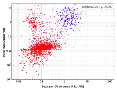
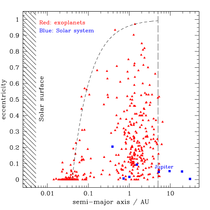
Figure 1 shows the distribution of a sample of extrasolar planets as a function of mass and orbital radius. Several thousand planets have been discovered from radial velocity surveys and transit searches, with NASA’s Kepler mission contributing the largest numbers. Direct imaging and microlensing searches have found smaller numbers of systems, but among them are some of particular interest for constraining planet formation theory. Despite this bonanza, it is clear from Figure 1 that large regions of parameter space remain to be explored. There is, to give one example, no current method that can find an extrasolar analog of Saturn, which plays a significant role in Solar System dynamics.
I.2.1 Radial velocity searches
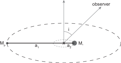
The observable in a radial velocity search for extrasolar planets is the time dependence of the radial velocity of a star due to the presence of an orbiting planet. For a planet on a circular orbit the geometry is shown in Figure 2. The star orbits the center of mass with a velocity,
| (6) |
Observing the system at an inclination angle , we see the radial velocity vary with a semi-amplitude ,
| (7) |
If the inclination is unknown, what we measure () determines a lower limit to the planet mass . Note that is not determined from the radial velocity curve, but must instead be determined from the stellar spectral properties. If the planet has an eccentric orbit, can be determined by fitting the non-sinusoidal radial velocity curve.
The noise sources for radial velocity surveys comprise photon noise, intrinsic jitter in the star (e.g. from convection or stellar oscillations), and instrumental effects. The magnitude of these effects vary (sometimes dramatically) from star to star. However, if we imagine an idealized survey for which the noise per observation was a constant, then the selection limit would be defined by,
| (8) |
with a constant. Planets with masses below this threshold would be undetectable, as would planets with orbital periods exceeding the duration of the survey (since orbital solutions are poorly constrained when only part of an orbit is observed unless the signal to noise of the observations is very high). The effect of such a selection boundary is evident in the distribution of the blue points in Figure 1. It favors the detection of low mass planets at small orbital radii, and has a relatively sharp cutoff beyond about 5 AU.

Extremely accurate radial velocity measurements are a prerequisite for discovering planets via this technique. For the Solar System,
| (9) |
Given that astronomical spectrographs have a resolving power of the order of (which corresponds, in velocity units, to a precision of the order of kilometers per second) it might seem impossible to find planets with such small radial velocity signatures. To appreciate how detection of small (sub-pixel) shifts is possible, it is useful to consider the precision that is possible against the background of shot noise (i.e. uncertainty in the number of photons due purely to counting statistics). An estimate of the photon noise limit can be derived by considering a very simple problem: how accurately can velocity shifts be estimated given measurement of the flux in a single pixel on the detector? To do this, we follow the basic approach of Butler et al. (1996) and consider the spectrum in the vicinity of a spectral line, as shown in Figure 3. Assume that, in an observation of some given duration, photons are detected in the wavelength interval corresponding to the shaded vertical band. If we now imagine displacing the spectrum by an amount (in velocity units) the change in the mean number of photons is,
| (10) |
Since a 1 detection of the shift requires that , the minimum velocity displacement that is detectable is,
| (11) |
This formula makes intuitive sense – regions of the spectrum that are flat are useless for measuring while sharp spectral features are good. For Solar-type stars with photospheric temperatures the sound speed at the photosphere is around 10 kms-1. Taking this as an estimate of the thermal broadening of spectral lines, the slope of the spectrum is at most,
| (12) |
Combining Equations (11) and (12) allows us to estimate the photon-limited radial velocity precision. For example, if the spectrum has a signal to noise ratio of 100 (and there are no other noise sources) then each pixel receives photons and . If the spectrum contains such pixels the combined limit to the radial velocity precision is,
| (13) |
Obviously this discussion ignores many aspects that are practically important in searching for planets from radial velocity data. However, it suffices to reveal the key feature: given a high signal to noise spectrum and stable wavelength calibration, photon noise is small enough that a radial velocity measurement with the ms-1 precision needed to detect extrasolar planets is feasible.
Records for the smallest amplitude radial velocity signal that can be extracted from the noise have improved dramatically over the years. Planets have now been detected for which is as small as about 0.5 (Pepe et al., 2011), and there are plans (e.g. the ESPRESSO instrument on ESO’s VLT) for next-generation instruments able to reach the 0.1 precision needed to find Earth analogs. It is important to remember that these are best-case values – many stars are not stable enough to allow anything like such high precision and complete samples of extrasolar planets that are suitable for statistical studies only exist for much larger .
Detailed modeling is necessary in order to assess whether a particular survey has a selection bias in eccentricity. Naively you can argue it either way – an eccentric planet produces a larger perturbation at closest stellar approach, but most of the time the planet is further out and the radial velocity is smaller. A good starting point for studying these issues is the explicit calculation for the Keck Planet Search reported by Cumming et al. (2008). These authors find that the Keck search is complete for sufficiently massive planets (and thus trivially unbiased) for .
I.2.2 Transit searches
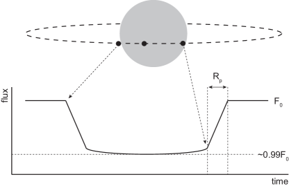
The observable for transit surveys is the stellar flux as a function of time. Planets emit very little flux in the visible, so to a good approximation a transiting planet produces the “U-shaped” light curve that would result from a perfectly obscuring disk moving across the stellar surface as seen from Earth. Simple geometrical considerations, illustrated in Figure 4, allow us to deduce two important facts. The transit depth (the fraction of the stellar flux that is blocked by the planet) is,
| (14) |
where and are the planetary and stellar radii. For giant planets the depth is of the order of 1%, while for the Earth around a Solar type star . To see a transit requires a favorable, almost edge-on, orbital alignment. For a planet at orbital radius , in a system observed at inclination angle , some part of the planet will touch the stellar disk provided that . Given random inclinations, the probability of transit is then,
| (15) |
For an Earth analog this is about 0.5%. As with radial velocity surveys, transit searches are thus strongly biased toward small orbital radii. Once planets are observed to transit, the measurable properties are the orbital period and the ratio of the planetary to stellar radius. The semi-major axis and planetary radius follow provided that the stellar mass and radius are known to good precision.
Transit searches have to contend with both noise and false positives — astronomical events unrelated to planets that masquerade as transit signals (eclipsing binaries whose light is blended with an unrelated third star are a major source of the latter). For ground-based transit searches the dominant noise component is atmospheric fluctuations, which make it hard to measure stellar fluxes to a fractional precision better than around the level. For Solar-type stars this restricts ground-based detections to the regime of gas or ice giants. (Low-mass stars’ smaller radii allow the detection of smaller planets, with GJ1214b having ; Charbonneau et al., 2009). From space, depending on the aperture of the telescope and the brightness of the target, some combination of photon noise and intrinsic stellar variability dominates the noise budget. Analyses of Kepler data by Gilliland et al. (2012) and Basri, Walkowicz & Reiners (2012) come to somewhat different conclusions, but are consistent with the broad-brush statement that the Sun’s noise level is somewhere between typical and moderately quiescent as compared to other Solar-type stars. The measured stellar noise levels (when added to photometric and instrumental noise sources) allowed Kepler to discover large numbers of small planets, though the realized precision and limited lifetime of the original mission proved to be marginal for the original goal of measuring the frequency of Earth-like planets at 1 AU around Solar-type stars.
The information yielded by transit detections can be increased in various special circumstances. The observation of multiple transit signals for a single target star provides, first, near-certainty that the photometric signal is genuinely caused by a planet rather than being a spurious false positive (because the probability of multiple false positive signals, with different periods, afflicting one star is very small; Lissauer et al., 2012). Second, if the planets producing the multiple transit signals are relatively closely spaced, their mutual gravitational perturbations may give rise to measurable Transit Timing Variations (TTVs) (Agol et al., 2005; Holman & Murray, 2005). The strength of TTVs is a (complex) function of the planets’ masses and orbital elements, but in a useful subset of cases enough information is available to constrain the planets’ masses using transit data alone (Ford et al., 2012). This is particularly important for the Kepler systems around faint hosts, where precision radial velocity follow-up is difficult and time-consuming.
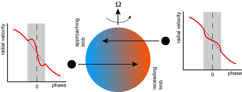
When radial velocity data is available for a star with one or more transiting planets it is immediately possible to estimate the true mass and density of the planets. Less obviously, with sufficiently precise radial velocity data it is possible to determine whether the transiting planet orbits within the plane defined by the rotating star’s equator. This is possible because, as shown in Figure 5, an extra radial velocity perturbation is produced as the planet obscures rotationally red-shifted or blue-shifted portions of the stellar photosphere. When this effect, known as the Rossiter-McLaughlin effect (Rossiter, 1924; McLaughlin, 1924)444The physical principles at work here long precede the detection of extrasolar planets. Detections of the “rotational effect” (as it was then called) in eclipsing binaries were published by Richard Rossiter (as part of his Ph.D. studying the beta Lyrae system), and by Dean McLaughlin (who studied Algol). Frank Schlesinger, and possibly others, may have seen similar effects in binaries., can be measured, it is possible to determine the sky-projected angle between the orbital angular momentum vector of the planet and the spin vector of the star. Although this is not the true inclination angle of the orbit, it nonetheless provides very useful information that can be used to test theories for the formation of close-in planetary systems.
I.2.3 Other exoplanet search methods
Several other search techniques, although less important for our current understanding of the exoplanet population, have either furnished unique information or have significant future discovery potential.
Gravitational microlensing, which works by detecting the planetary perturbation to the light curve of a distant star lensed by a foreground planet host, is the ground-based technique with the best sensitivity to low-mass planets. A planet with a mass of roughly was found with this technique more that a decade ago (Beaulieu et al., 2006). The method is most sensitive to planets orbiting near the Einstein ring radius (the radius at which light from the background star traverses the lens system en route to us) which, interestingly, is at about the radius of the snow line (a few AU). A review of the method and results can be found in Gaudi (2010). NASA’s proposed WFIRST mission would be able to detect a large number of low-mass planets via this technique.
Direct imaging is presently not competitive as a means of discovering planets that would be analogs of the Solar System’s terrestrial or giant planets, but is sensitive enough to detect massive planets at larger orbital radii. From a theoretical viewpoint, by far the most interesting system seen to date is that surrounding HR 8799 (Marois et al., 2008, 2010). The system has four very massive planets orbiting at projected radii that extend out to 70 AU. As we will discuss later, it is hard to see how such a system could form in situ. Existing survey results show that systems similar to HR 8799 are moderately rare (occurring with a frequency of the order of 1%; Galicher, 2016), but the error bars are large. An improvement is expected with results from surveys using newer instruments, including the Gemini Planet Imager and VLT Sphere.
Astrometry works in conceptually exactly the same way as radial velocity surveys, except that the observable is the variation of the two-dimensional position of the star in the plane of the sky rather than the one-dimensional line of sight velocity. The GAIA mission, currently flying, is expected to discover a large number of planets via this technique.
I.3 Exoplanet properties
The time has long since passed when a few pages could summarize what is known observationally about extrasolar planetary systems. Here, we summarize some of their basic properties and highlight a few of the open issues that seem especially relevant to planet formation theory.
I.3.1 Planetary masses and radii
The mass distribution of extrasolar planets has been well-constrained by radial velocity surveys across the range of masses associated with ice and gas giants. An analysis of data from 2,500 stars targeted as part of the Lick / Keck / AAT survey identified 250 planets, distributed in mass and radius as (Marcy et al., 2008),
| (16) | |||
| (17) |
Relatively few planets with orbital radii beyond 5 AU are known, but with that caveat the observed mass distribution between about 5 and 10 can be considered reliably determined (compare the above analysis, for example, to earlier work by Tabachnik & Tremaine, 2002). A relatively modest extrapolation suggests that around 20% of Solar-type stars are orbited by giant planets with semi-major axis less than 20 AU (Marcy et al., 2008). Most of these planets are not part of the hot Jupiter systems that were the first to be discovered, but rather orbit at larger distances from their hosts.
The most surprising result from the Kepler mission has been the discovery of a very large population of small planets in short-period orbits. For periods and , for example, Youdin (2011) estimate the number of planets per star to be around unity (). As with the radial velocity sample, these planets are smoothly distributed in size with a distribution that increases steeply toward small radii. Howard et al. (2012) found that for planets interior to 0.25 AU the size distribution followed,
| (18) |
down to radii . Intriguingly, the data does not display a bimodal distribution of sizes, as might be expected based on the clear separation between the radii of Solar System terrestrial and giant planets. Below there is a decrease in the slope of the size distribution, which may be roughly flat between Petigura, Marcy & Howard (2013).
Masses (and hence mean densities) are only available for the small subset of the Kepler sample that have precision Doppler measurements or useful transit timing variation constraints. It is clear, however, that the “mid-sized” Kepler planets form a heterogeneous sample containing both “super-Earths” (rocky planets with masses and radii greater than the Earth) and “mini-Neptunes” (planets with cores but also substantial gaseous envelopes). The Kepler-36 system, for example, contains two planets in adjacent orbits, one with a mass of and a density of , and the other with a mass of and a density of (Carter et al., 2012). Analysis and follow-up of the Kepler data is ongoing, but current work is consistent with a picture where planets with are predominantly super-Earths, while samples of larger planets contain a rising population of mini-Neptunes (Weiss & Marcy, 2014; Marcy et al., 2014).
I.3.2 Orbital properties
The distribution of giant planets in the - plane is shown in Figure 6, using a sample of data taken from the exoplanets.org database. The closest-in hot Jupiters have circular orbits, due to tidal dissipation in the star and planet555Using a tidal model Hansen (2010) fits a circularization period of about 3 days to similar data.. At larger radii, however, the observed sample of exoplanets shows a striking spread in eccentricity. The median eccentricity is , and some extremely eccentric planets exist with . One should bear in mind that most of the detected planets are at smaller orbital radius than any of the gas giants in the Solar System, and many are more massive. Nonetheless, these large eccentricities are strikingly unlike the near-circular orbits that we are familiar with.
Several properties of observed giant planet systems are considered to furnish clues to the origin of eccentricity and hot Jupiters. One is the fact that “hot Jupiters are (almost always) alone”. Around stars that do not have a hot Jupiter, detections of multiple giant planets are reasonably common, with Hartman et al. (2014) quoting an abundance of 22% (this number is evidently affected by many selection effects, so its absolute value is not important). In contrast, those systems with a hot Jupiter (defined as ) have an abundance of detected companions that is only around 3%. A qualitatively similar result holds true for lower mass companions to hot Jupiters (Steffen et al., 2012). This paucity of nearby companions suggests that the formation process of hot Jupiters is most often inconsistent with the formation or survival of another close-in planet.
An independent clue to hot Jupiter origins comes from measurements of the Rossiter-McLaughlin effect for transiting hot Jupiters. Winn et al. (2012) found that hot Jupiters orbiting stars with effective temperatures showed a broad distribution of projected obliquities, including some systems with polar and retrograde orbits. Cooler stars, on the other hand, showed a greater preponderance of aligned planetary orbits. The current obliquities may well be affected by tidal evolution — complicating quantitative comparisons — but the existence of some highly misaligned hot Jupiters certainly suggests that the formation process knew nothing about the spin axis of the star.
The prevalence of resonant planetary systems is also of interest. An early example was the GJ 876 system, which contains two massive planets in a 2:1 mean motion resonance. Unfortunately, an iron-clad determination of resonant behavior in an exoplanet system requires detailed observations that are not available for all known multi-planet systems. Among the best-characterized multi-planet systems containing gas giants, however, resonant configurations appear to be common. Wright et al. (2011), for example, estimate a resonant fraction of around a third. As in the Solar System, the existence of these resonances is taken as evidence for dissipative processes occurring during the evolution of the system (Lee & Peale, 2002).
The above discussion of resonances applies to giant planet systems discovered via radial velocity surveys. The period ratios observed in multiple planet Kepler systems show a subtle, but even more intriguing structure. Most Kepler multiple systems are non-resonant, but there is a significant excess of pairs that are just outside first order MMRs such as the 2:1 and 3:2 (Fabrycky et al., 2014). This result is not easy to interpret, as it seems to imply simultaneously that these planets are influenced by resonant effects while avoiding the large-scale trapping into resonance that would be the simplest prediction of gas disk migration models. The short assembly time scale of planets in close-in orbits means that the effects of gas disk migration are likely significant, and hence one idea is that a higher fraction of primordial resonances has been subsequently disrupted. A broad range of theoretical ideas have been studied, but there is no consensus as to the most important physical processes responsible for the observed Kepler systems. Paper that discuss various aspects of the problem include Petrovich, Malhotra & Tremaine (2013), Goldreich & Schlichting (2014), Hands, Alexander & Dehnen (2014), Chatterjee & Ford (2015), Pu & Wu (2015) and Coleman & Nelson (2016).
I.3.3 Host properties

The dependence of giant planet frequency with stellar metallicity is shown in Figure 7, using data from the paper by Fischer & Valenti (2005). A strong trend is evident. Changes in metallicity of a factor of a few lead to large variations in the incidence of detected giant planets. This is not surprising. Within the core accretion model for giant planet formation, a prerequisite for forming a gas giant is the ability to assemble a solid core of during the few million year lifetime of the gas disk, and this is evidently easier to fulfill if the total inventory of disk solids is boosted. The same is not true of lower mass planets. Sousa et al. (2008) found that the abundance of Neptune analogs is not a strong function of host metallicity, and Everett et al. (2013), and other groups, find that the same is true of the smaller planets in the Kepler sample. These results suggest that even if critical stages of planet formation — such as the formation of planetesimals — require threshold levels of metallicity (as suggested by, e.g., Johansen, Youdin & Mac Low, 2009), it is still possible for stars with moderately sub-Solar metallicity to form systems of lower-mass planets.
The frequency of relatively close-in planets has been measured as a function of stellar type from Kepler data. Howard et al. (2012) find that planets with radii of are substantially (by a factor of 7) more abundant around the coolest stars () than around stars with . I am not aware of a simple explanation for this trend.
Kepler data has also identified a small number of circumbinary planets (Doyle et al., 2011; Welsh et al., 2012), whose properties are consistent with low mass gas giants. Estimates suggest that of the order of 1% of tight binaries have such gas giants in almost coplanar orbits, so these are not particularly rare systems. They are particularly interesting for planet formation because gravitational perturbations from the binary would have increased the collision velocities of planetesimals above the values seen around single stars, making it harder for cores to grow in situ (Lines et al., 2014, and references therein).
I.3.4 Planetary structure
Empirical determination of the planetary mass-radius relation (from a combination of transit measurements of the radius, and radial velocity or TTV determinations of the mass) provides a test of models for planetary structure. To leading order the expectation for gas giants is that the mass-radius relation ought to be flat, with being a decent approximation for sub-Jovian to several Jupiter mass planets. Actual transit data, however, shows that hot Jupiter radii scatter substantially above and below the expected values. The undersized gas giants are interesting, but pose no special theoretical conundrum. To first order, the radius of a gas giant of a given mass varies with the total mass of heavy elements it contains666Whether those heavy elements are distributed evenly within the planet or concentrated at the center in a core also affects the radius, but at a more subtle level.; hence a plausible explanation for any small planet is that it has an above-average heavy element content. The measured radius of the Saturn mass planet orbiting HD 149026, for example, is generally interpreted as providing evidence for approximately of heavy elements in the interior (Sato et al., 2005). The inflated planets, on the other hand, are more mysterious, since some (examples include TrES-4 and WASP-12b) are too large even when compared to pure hydrogen / helium models. Explaining their radii requires an additional source of heat.
The origin of the heat source needed to explain inflated hot Jupiter radii is not fully understood, and may not be unique. Empirically it is observed that the prevalence of inflated radii increases with the degree of stellar irradiation (see, e.g., plots in Demory & Seager, 2011; Spiegel & Burrows, 2013), suggesting that in at least some cases stellar heating can couple into the convective interior efficiently enough to impact the radius. Suggestions for how this coupling might be realized physically include substantial changes to atmospheric opacities (Burrows et al., 2007), waves that connect the radiative and convective regions (Guillot & Showman, 2002), and magnetic fields that generate Ohmic heating of the interior (Batygin & Stevenson, 2010; Ginsburg & Sari, 2016). Spiegel & Burrows (2013) provide a much more extensive list of references to proposed mechanisms.
The composition of lower mass planets is plausibly much more diverse. In the Solar System we have have only the terrestrial planets (dominated by rock, with atmospheres that are negligible from a mass-radius perspective) and the ice giants, but the results from Kepler show that the Solar System gap between these classes is not a general outcome of planet formation. Taking generality to its extreme limit, we might then consider the structure of low-mass planets composed of arbitrary mixtures of iron, silicates, ices and H/He. This approach yields instructive limits: an inferred density higher than that of a pure iron planet is unphysical, while a density lower than that of a pure silicate world implies the existence of an atmosphere of volatiles. An analysis by Rogers (2015) suggests that most Kepler planets larger than have transit radii that are determined by their atmospheres or envelopes. It is clear, of course, that there are normally too many variables to admit a unique determination of the composition given only measurements of the mass and radius, and other constraints are needed to break degeneracies. Such constraints could come from additional observations (e.g. of the atmospheric composition) or from theoretical priors (e.g. a 100% water planet is hard to construct outside of science fiction).
I.3.5 Habitability
The primary long-term goal of observational exoplanet research is to identify low-mass planets and characterize their atmospheres via either transmission or emission spectroscopy. We currently know almost nothing about the diversity of terrestrial planet atmospheres, so such an exercise is certain to be scientifically interesting. Moreover, it is possible that we might identify one or more biomarkers — atmospheric constituents that have a biological origin on Earth and which would be removed from the atmosphere by abiotic processes on a short time scale. Oxygen is much the most important of these. If it proves possible both to measure one or more biomarkers, and to robustly exclude non-biological interpretations, we will have discovered evidence for life elsewhere.
In the current absence of such empirical evidence, the best we can do is to make educated guesses as to which extrasolar planets have the best chance of being habitable. Habitability is not a precisely defined concept, and discussion of it invites speculation as to which planetary properties are either essential or favorable for life. On the Earth, for example, we owe the long-term stability of the climate to the negative feedback of the carbonate-silicate cycle, by which the volcanic outgassing of greenhouse gases is balanced against the temperature-dependent weathering of silicate rocks (Walker, Hays & Kasting, 1981). The operation of this cycle requires plate tectonics, which then may (or may not) be a prerequisite for habitability. Similarly, magnetic fields — which reduce the rate of atmospheric erosion due to high energy radiation — and a stable obliquity have been suggested to contribute to the Earth’s benign environment.
The prospects for remotely measuring all of the properties that might impact habitability are slim. We can, however, plausibly identify planets whose temperatures and pressures could support liquid water on their surfaces. The presence of liquid water on the surface is probably neither a necessary nor a sufficient condition for a planet to be habitable (note that in the Solar System, there is interest in moons such as Europa that likely support sub-surface oceans), but by convention the range of orbital radii across which planets on circular orbits could maintain surface water is called the habitable zone (Kasting, Whitmire & Reynolds, 1993). The habitable zone varies with both time (the young Sun was as much as 30% fainter than it is today; Sagan & Mullen, 1972) and planetary mass (Kopparapu et al., 2014). The uncertain role of greenhouse gases means that even this simplest element of habitability is not easy to calculate accurately. Let us first consider a planet devoid of any atmosphere. Balancing incoming stellar radiation against outgoing thermal radiation gives, for a planetary albedo ,
| (19) |
This estimate gives a temperature significantly lower than the actual temperature when applied to the Earth (taking ). Clearly, an accounting for the warming effects of the atmosphere is essential.
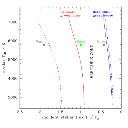
Two approaches have been used to estimate the extent of the habitable zone. The theoretical approach, pioneering by Kasting, Whitmire & Reynolds (1993), uses planetary atmosphere models to bracket the conditions under which a greenhouse gas atmosphere can sustain liquid water on the surface. The inner edge of the habitable zone is set by the onset of a runaway greenhouse, in which increased surface temperatures lead to increased evaporation of surface water (itself a greenhouse gas), so that the entire ocean inventory of water ultimately ends up in the atmosphere. The outer edge is set by a maximum greenhouse condition. Although a volcanic planet can outgas very large quantities of CO2, the maximum atmospheric content (and consequently the maximum extent of warming) is limited by the onset of CO2 condensation. Figure 8 shows the width of the habitable zone defined theoretically by these physical considerations (Kopparapu et al., 2013).
The theoretical habitable zone is not very broad. For current Solar conditions the inner edge is not far inside 1 AU, while the outer extent would not stretch to encompass the orbit of Mars given the faintness of the young Sun. As discussed in the review by Güdel et al. (2014) it is likely that the true habitable zone differs from the idealized theoretical one, due to known simplifications (e.g. using one dimensional atmosphere models) and, possibly, neglected physical effects. It is then useful to consider an empirical habitable zone defined, not by theory, but rather by Solar System observations. There is both in situ and geomorphological evidence that liquid water flowed on Mars around 4 Gyr ago, suggesting but not proving that Mars lay inside the outer edge of the habitable zone despite the lower Solar flux at that time. Less securely, there are suggestions that Venus may have been habitable in the relatively recent past, even though it is well inside the theoretical inner boundary of the habitable zone. From these considerations we can define an empirical habitable zone for the Solar System and, by appropriate scaling, for other stellar types. These limits, which are shown as the dashed lines in Figure 8, can be regarded as optimistic inner and outer bounds.
II Protoplanetary Disks
A more extensive review of protoplanetary disk physics can be found in “Physical processes in protoplanetary disks” (Armitage, 2015). The reader whose main interests lie in disks may want to start there.
II.1 The star formation context
Stars form in the Galaxy today from the small fraction of gas that exists in dense molecular clouds. Molecular clouds are observed in one or more molecular tracers – examples include CO, 13CO and NH3 – which can be used both to probe different regimes of column density and to furnish kinematic information that can give clues as to the presence of rotation, infall and outflows. Observations of the dense, small scale cores within molecular clouds (with scales of the order of 0.1 pc) that are the immediate precursors of star formation show velocity gradients that are of the order of . Even if all of such a gradient is attributed to rotation, the parameter,
| (20) |
is small – often of the order of 0.01. Hence rotation is dynamically unimportant during the early stages of collapse. The angular momentum, on the other hand, is large, with a ballpark figure being . This is much larger than the angular momentum in the Solar System, never mind that of the Sun, a discrepancy that is described as the angular momentum problem of star formation. The problem has multiple solutions. Many stars are part of binary systems with large amounts of orbital angular momentum. For the single stars, magnetic flux that is approximately conserved within the collapsing gas can remove angular momentum from the system (this process can be too efficient, resulting in a “magnetic braking catastrophe” that precludes disk formation; Li et al., 2014). For our purposes, it suffices to note that the specific angular momentum of gas in molecular cloud cores would typically match the specific angular momentum of gas in Keplerian orbit around a Solar mass star at a radius of AU.
The observed properties of molecular cloud cores are thus consistent with the formation of large disks – of the size of the Solar System and above – around newly formed stars. At least initially, those disks could be quite massive. One would also expect the disks to retain some net magnetic field that is a residual of the complex fields that likely threaded the molecular cloud core.
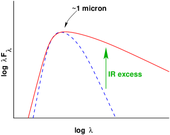
Young Stellar Objects (YSOs) are classified observationally according to the shape of their Spectral Energy Distribution in the infra-red. As shown schematically in Figure 9, YSOs often display,
-
1.
An infra-red excess (over the stellar photospheric contribution) that is attributed to hot dust in the disk near the star.
-
2.
An ultra-violet excess, which is ascribed to high temperature regions (probably hot spots) on the stellar surface where gas from the disk is being accreted.
To quantify the magnitude of the IR excess, it is useful to define a measure of the slope of the IR SED,
| (21) |
between the near-IR and the mid-IR. Conventions vary, but for illustration we can assume that the slope is measured between the K band (at 2.2) and the N band (at 10). We can then classify YSOs as,
-
•
Class 0: SED peaks in the far-IR or mm part of the spectrum (), with no flux being detectable in the near-IR.
-
•
Class I: approximately flat or rising SED into mid-IR ().
-
•
Class II: falling SED into mid-IR (). These objects are also called “Classical T Tauri stars”.
-
•
Class III: pre-main-sequence stars with little or no excess in the IR. These are the “Weak lined T Tauri stars” (note that although WTTs are defined via the equivalent width of the H line, this is an accretion signature that correlates well with the presence of an IR excess).
This observational classification scheme is theoretically interpreted, in part, as an evolutionary sequence (Adams, Lada & Shu, 1987). In particular, clearly objects in Classes 0 through II eventually lose their disks and become Class III sources. Observational estimates for the duration of the gas disk phase are typically a few Myr (Haisch, Lada & Lada, 2001). While the gas is present, however, viewing angle may well play a role in determining whether a given source is observed as a Class I or Class II object.
II.2 Passive circumstellar disks
An important physical distinction needs to be drawn between passive circumstellar disks, which derive most of their luminosity from reprocessed starlight, and active disks, which are instead powered by the release of gravitational potential energy as gas flows inward. For a disk with an accretion rate , surrounding a star with luminosity and radius , the critical accretion rate below which the accretion energy can be neglected may be estimated as,
| (22) |
where we have anticipated the result, derived below, that a flat disk intercepts one quarter of the stellar flux. Numerically,
| (23) |
Measured accretion rates of Classical T Tauri stars (Gullbring et al., 1998) range from an order of magnitude above this critical rate to two orders of magnitude below, so it is oversimplifying to assume that protoplanetary disks are either always passive or always active. Rather, the dominant source of energy for a disk is a function of both time and radius. We expect internal heating to dominate at early epochs and / or small orbital radii, while at late times and at large radii reprocessing dominates.
II.2.1 Vertical structure
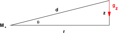
The vertical structure of a geometrically thin disk (either passive or active) is derived by considering vertical hydrostatic equilibrium (Figure 10). The pressure gradient is,
| (24) |
where is the gas density. Ignoring any contribution to the gravitational force from the disk (this is justified provided that the disk is not too massive), the vertical component of gravity seen by a parcel of gas at cylindrical radius and height above the midplane is,
| (25) |
For a thin disk , so
| (26) |
where is the Keplerian angular velocity. If we assume for simplicity that the disk is vertically isothermal (this will be a decent approximation for a passive disk, less so for an active disk) then the equation of state is , where is the (constant) sound speed. The equation of hydrostatic equilibrium (equation 24) then becomes,
| (27) |
The solution is,
| (28) |
where and , the vertical scale height, is given by,
| (29) |
Integrating equation (28) over , we can write the mid-plane density in terms of the surface density and vertical scale height,
| (30) |
We can also compare the disk thickness to the radius,
| (31) |
where is the local orbital velocity. We see that the aspect ratio of the disk is inversely proportional to the Mach number of the flow.
The shape of the disk depends upon . If we parameterize the radial variation of the sound speed via,
| (32) |
then the aspect ratio varies as,
| (33) |
The disk will flare – i.e. will increase with radius giving the disk a bowl-like shape – if . This requires a temperature profile or shallower. As we will show shortly, flaring disks are expected to be the norm.
II.2.2 Radial temperature profile
The physics of the calculation of the radial temperature profile of a passive disk is described in papers by Adams & Shu (1986), Kenyon & Hartmann (1987) and Chiang & Goldreich (1997). We begin by considering the absolute simplest model: a flat thin disk in the equatorial plane that absorbs all incident stellar radiation and re-emits it as a single temperature blackbody. The back-warming of the star by the disk is neglected.
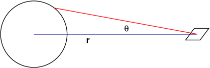
We consider a surface in the plane of the disk at distance from a star of radius . The star is assumed to be a sphere of constant brightness . Setting up spherical polar co-ordinates, as shown in Figure 11, the stellar flux passing through this surface is,
| (34) |
We count the flux coming from the top half of the star only (and to be consistent equate that to radiation from only the top surface of the disk), so the limits on the integral are,
| (35) |
Substituting , the integral for the flux is,
| (36) |
which evaluates to,
| (37) |
For a star with effective temperature , the brightness , with the Stefan-Boltzmann constant (Rybicki & Lightman, 1979). Equating to the one-sided disk emission we obtain a radial temperature profile,
| (38) |
Integrating over radii, we obtain the total disk flux,
| (39) | |||||
We conclude that a flat passive disk extending all the way to the stellar equator intercepts a quarter of the stellar flux. The ratio of the observed bolometric luminosity of such a disk to the stellar luminosity will vary with viewing angle, but clearly a flat passive disk is predicted to be less luminous than the star.
The form of the temperature profile given by equation (38) is not very transparent. Expanding the right hand side in a Taylor series, assuming that (i.e. far from the stellar surface), we obtain,
| (40) |
as the limiting temperature profile of a thin, flat, passive disk. For fixed molecular weight this in turn implies a sound speed profile,
| (41) |
Assuming vertical isothermality, the aspect ratio given by equation (33) is,
| (42) |
and we predict that the disk ought to flare modestly to larger radii. If the disk does flare, then the outer regions intercept a larger fraction of stellar photons, leading to a higher temperature. As a consequence, a temperature profile is probably the steepest profile we would expect to obtain for a passive disk.
II.2.3 Spectral energy distribution (SED)
Suppose that each annulus in the disk radiates as a blackbody at the local temperature . If the disk extends from to , the disk spectrum is just the sum of these blackbodies weighted by the disk area,
| (43) |
where is the Planck function,
| (44) |
The behavior of the spectrum implied by equation (43) is easy to derive. At long wavelengths we recover the Rayleigh-Jeans form,
| (45) |
while at short wavelengths there is an exponential cut-off that matches that of the hottest annulus in the disk,
| (46) |
For intermediate wavelengths,
| (47) |
the form of the spectrum can be found by substituting,
| (48) |
into equation (43). We then have, approximately,
| (49) |
and so
| (50) |
The overall spectrum, shown schematically in Figure 12, is that of a “stretched” blackbody (Lynden-Bell, 1969).
The SED predicted by this simple model generates an IR-excess, but with a declining SED in the mid-IR. This is too steep to match the observations of even most Class II sources.
II.2.4 Sketch of more complete models
Two additional pieces of physics need to be included when computing detailed models of the SEDs of passive disks. First, as already noted above, all reasonable disk models flare toward large , and as a consequence intercept and reprocess a larger fraction of the stellar flux. At large radii, Kenyon & Hartmann (1987) find that consistent flared disk models approach a temperature profile,
| (51) |
which is much flatter than the profile derived previously. Second, the assumption that the emission from the disk can be approximated as a single blackbody is too simple. In fact, dust in the surface layers of the disk radiates at a significantly higher temperature because the dust is more efficient at absorbing short-wavelength stellar radiation than it is at emitting in the IR (Shlosman & Begelman, 1989). Dust particles of size absorb radiation efficiently for , but are inefficient absorbers and emitters for (i.e. the opacity is a declining function of wavelength). As a result, the disk absorbs stellar radiation close to the surface (where ), where the optical depth to emission at longer IR wavelengths . The surface emission comes from low optical depth, and is not at the blackbody temperature previously derived. Chiang & Goldreich (1997) showed that a relatively simple disk model made up of,
-
1.
A hot surface dust layer that directly re-radiates half of the stellar flux
-
2.
A cooler disk interior that reprocesses the other half of the stellar flux and re-emits it as thermal radiation
can, when combined with a flaring geometry, reproduce most SEDs quite well. A review of recent disk modeling work is given by Dullemond et al. (2007).
The above considerations are largely sufficient to understand the structure and SEDs of Class II sources. For Class I sources, however, the possible presence of an envelope (usually envisaged to comprise dust and gas that is still infalling toward the star-disk system) also needs to be considered. The reader is directed to Eisner et al. (2005) for one example of how modeling of such systems can be used to try and constrain their physical properties and evolutionary state.
II.3 Actively accreting disks
The radial force balance in a passive disk includes contributions from gravity, centrifugal force, and radial pressure gradients. The equation reads,
| (52) |
where is the orbital velocity of the gas and is the pressure. To estimate the magnitude of the pressure gradient term we note that,
| (53) | |||||
where for the final step we have made use of the relation . If is the Keplerian velocity at radius , we then have that,
| (54) |
i.e pressure gradients make a negligible contribution to the rotation curve of gas in a geometrically thin disk777This is not to say that pressure gradients are unimportant – as we will see later the small difference between and is of critical importance for the dynamics of small rocks within the disk.. To a good approximation, the specific angular momentum of the gas within the disk is just that of a Keplerian orbit,
| (55) |
which is an increasing function of radius. To accrete on to the star, gas in a disk must lose angular momentum, either,
-
1.
Via redistribution of angular momentum within the disk (normally described as being due to “viscosity”, though this is a loaded term, best avoided where possible).
-
2.
Via loss of angular momentum from the star-disk system, for example in a magnetically driven disk wind.
Aspects of models in the second class have been studied for a long time – the famous disk wind solution of Blandford & Payne (1982), for example, describes how a wind can carry away angular momentum from an underlying disk. Observationally, it is not known whether magnetic winds are launched from protoplanetary disks on AU scales (jets, of course, are observed, but these are probably launched closer to the star), and hence the question of whether winds are important for the large-scale evolution of disks remains open. An review of the theory of disk winds as applied to protostellar systems is given by Königl & Salmeron (2011), while Bai et al. (2016) present wind models, motivated by recent simulations, that incorporate both magnetic and thermal driving. To get started though, we’ll initially assume that winds are not the dominant driver of evolution, and derive the equation for the time evolution of the surface density for a thin, viscous disk (Lynden-Bell & Pringle, 1974; Shakura & Sunyaev, 1973). Clear reviews of the fundamentals of accretion disk theory can be found in Pringle (1981) and in Frank, King & Raine (2002).
II.3.1 Diffusive evolution equation
Let the disk have surface density and radial velocity (defined such that for inflow). The potential is assumed fixed so that the angular velocity only. In cylindrical co-ordinates, the continuity equation for an axisymmetric flow gives (see e.g. Pringle (1981) for an elementary derivation),
| (56) |
Similarly, conservation of angular momentum yields,
| (57) |
where the term on the right-hand side represents the net torque acting on the fluid due to viscous stresses. From fluid dynamics (Pringle, 1981), is given in terms of the kinematic viscosity by the expression,
| (58) |
where the right-hand side is the product of the circumference, the viscous force per unit length, and the level arm . If we substitute for , eliminate between equation (56) and equation (57), and specialize to a Keplerian potential with , we obtain the evolution equation for the surface density of a thin accretion disk in its normal form,
| (59) |
This partial differential equation for the evolution of the surface density has the form of a diffusion equation. To make that explicit, we change variables to,
| (60) |
For a constant , equation (59) then takes the prototypical form for a diffusion equation,
| (61) |
with a diffusion coefficient,
| (62) |
The characteristic diffusion time scale implied by equation (61) is . Converting back to the physical variables, we find that the evolution time scale for a disk of scale with kinematic viscosity is,
| (63) |
Observations of disk evolution (for example determinations of the time scale for the secular decline in the accretion rate) can therefore be combined with estimates of the disk size to yield an estimate of the effective viscosity in the disk (Hartmann et al., 1998).
II.3.2 Solutions
In general is expected to be some function of the local conditions within the disk (surface density, radius, temperature, ionization fraction etc). If depends on , then equation (59) becomes a non-linear equation with no analytic solution (except in some special cases), while if there is a more complex dependence on the local conditions then the surface density evolution equation will often need to be solved simultaneously with an evolution equation for the central temperature (Pringle, Verbunt & Wade, 1986). Analytic solutions are possible, however, if can be written as a power-law in radius (Lynden-Bell & Pringle, 1974), and these suffice to illustrate the essential behavior implied by equation (59).

First, we describe a Green’s function solution to equation (59) for the case . Suppose that at , all of the gas lies in a thin ring of mass at radius ,
| (64) |
One can show that the solution is then,
| (65) |
where we have written the solution in terms of dimensionless variables , , and is a modified Bessel function of the first kind.
Unless you have a special affinity for Bessel functions, this Green’s function solution is not terribly transparent. The evolution it implies is shown in Figure 13. The most important features of the solution are that, as ,
-
•
The mass flows to .
-
•
The angular momentum, carried by a negligible fraction of the mass, flows toward .
This segregation of mass and angular momentum is a generic feature of viscous disk evolution, and is obviously relevant to the angular momentum problem of star formation.

Of greater practical utility is the self-similar solution also derived by Lynden-Bell & Pringle (1974). Consider a disk in which the viscosity can be approximated as a power-law in radius,
| (66) |
Suppose that the disk at time has the surface density profile corresponding to a steady-state solution (with this viscosity law) out to , with an exponential cut-off at larger radii. As we will shortly show, the initial surface density then has the form,
| (67) |
where is a normalization constant, , and . The self-similar solution is then,
| (68) |
where,
| (69) |
This solution is plotted in Figure 14. Over time, the disk mass decreases while the characteristic scale of the disk (initially ) expands to conserve angular momentum. This solution is quite useful both for studying evolving disks analytically, and for comparing observations of disk masses, accretion rates or radii with theory (Hartmann et al., 1998).
A steady-state solution for the radial dependence of the surface density can be derived by setting and integrating the angular momentum conservation equation (57). This yields,
| (70) |
Noting that the mass accretion rate we have,
| (71) |
To determine the constant of integration, we note that the torque within the disk vanishes if . At such a location, the constant can be evaluated and is just proportional to the local flux of angular momentum
| (72) |
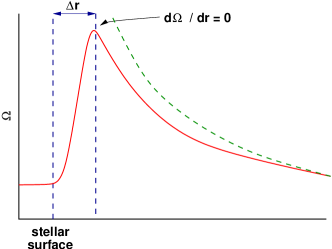
Usually this is determined at the inner boundary. A particularly simple example is the case of a disk that extends to the equator of a slowly rotating star. This case is illustrated in Figure 15. In order for there to be a transition between the Keplerian angular velocity profile in the disk and the much smaller angular velocity at the stellar surface there must be a maximum in at some radius . Elementary arguments (Pringle, 1977) – which may fail at the very high accretion rates of FU Orionis objects (Popham et al., 1993) but which are probably reliable otherwise – suggest that , so that the transition occurs in a narrow boundary layer close to the stellar surface. The constant can then be evaluated as,
| (73) |
and equation (71) becomes,
| (74) |
Given a viscosity, this equation defines the steady-state surface density profile for a disk with an accretion rate . Away from the boundaries, .
The origin of angular momentum transport within the boundary layer itself presents interesting complications, since the boundary layer is a region of strong shear that is stable against the magnetorotational instabilities that we will argue later are critical for transporting angular momentum within disks. As a consequence, magnetic field evolution is qualitatively different within the boundary layer as compared to the Keplerian disk (Pringle, 1989; Armitage, 2002). Analytic and simulation work by Belyaev, Rafikov & Stone (2013) shows that acoustic waves provide the dominant source of transport in the boundary layer region.
The inner boundary condition which leads to equation (74) is described as a zero-torque boundary condition. As noted, zero-torque conditions are physically realized in the case where there is a boundary layer between the star and its disk. This is not, however, the case in most Classical T Tauri stars. Observational evidence suggests (Bouvier et al., 2007) that in accreting T Tauri stars the stellar magnetosphere disrupts the inner accretion disk, leading to a magnetospheric mode of accretion in which gas becomes tied to stellar field lines and falls ballistically on to the stellar surface (Königl, 1991). The magnetic coupling between the star and its disk allows for angular momentum exchange, modifies the steady-state surface density profile close to the inner truncation radius, and may allow the star to rotate more slowly than would otherwise be the case (Collier Cameron & Campbell, 1993; Armitage & Clarke, 1996). Whether such “disk-locking” actually regulates the spin of young stars remains a matter of debate, however, and both theoretical and observational studies have returned somewhat ambiguous results (Matt & Pudritz, 2005; Herbst & Mundt, 2005; Rebull et al., 2006).
II.3.3 Temperature profile
Following Frank, King & Raine (2002), we derive the radial dependence of the effective temperature of an actively accreting disk by considering the net torque on a ring of width . This torque – – does work at a rate,
| (75) |
where . Written this way, we note that if we consider the whole disk (by integrating over ) the first term on the right-hand-side is determined solely by the boundary values of . We therefore identify this term with the transport of energy, associated with the viscous torque, through the annulus. The second term represents the rate of loss of energy to the gas. We assume that this is ultimately converted into heat and radiated, so that the dissipation rate per unit surface area of the disk (allowing that the disk has two sides) is,
| (76) |
where we have assumed a Keplerian angular velocity profile. For blackbody emission . Substituting for , and for using the steady-state solution given by equation (74), we obtain,
| (77) |
We note that,
-
•
Away from the boundaries , the temperature profile of an actively accreting disk is . This has the same form as for a passive disk given by equation (40).
-
•
The temperature profile does not depend upon the viscosity. This is an attractive feature of the theory given uncertainties regarding the origin and efficiency of disk angular momentum transport. On the flip side, it eliminates many possible routes to learning about the physics underlying via observations of steady-disks.
Substituting a representative value for the accretion rate of , we obtain for a Solar mass star at 1 AU an effective temperature . This is the surface temperature, as we will show shortly the central temperature is predicted to be substantially higher.
II.3.4 Shakura-Sunyaev disks
Molecular viscosity is negligible in protoplanetary disks. For a gas in which the mean free path is , the viscosity
| (78) |
where is the sound speed. In turn, the mean free path is given by , where is the number density of molecules with cross-section for collision . These quantities are readily estimated. For example, consider a protoplanetary disk with and at 1 AU. The midplane density is of the order of , while the sound speed implied by the specified is . The collision cross-section of a hydrogen molecule is of the order of Chapman & Cowling (1970),
| (79) |
and hence we estimate,
| (80) |
The implied disk evolution time scale then works out to be of the order of yr – at least times too slow to account for observed disk evolution.
In a classic paper Shakura & Sunyaev (1973) noted that turbulence within the disk can provide an effective viscosity that greatly exceeds molecular viscosity. For isotropic turbulence, the maximum scale of turbulent cells within the disk will be of the same order as the vertical scale height , while the maximum velocity of turbulent motions relative to the mean flow is comparable to the sound speed (any larger velocity would lead to shocks and rapid dissipation of turbulent kinetic energy into heat). Such considerations motivate a parameterization,
| (81) |
where is a dimensionless parameter that measures how efficient the turbulence is at creating angular momentum transport. We note at the outset that the existence of turbulence within the disk does not, a priori, guarantee that the outward angular momentum transport necessary to drive accretion will occur.
In the standard theory of so-called “-disks”, is treated as a constant. If this is done, it is possible to solve analytically for the approximate vertical structure of an actively accreting disk and derive a scaling for as a function of , and . Textbook discussions of this procedure can be found in Frank, King & Raine (2002), Armitage (2010), and many other places. Combining the known functional form for with the disk evolution equation (59) then yields a full theory for the predicted time dependence of the disk, with the only unknown being the appropriate value for . This is all very well, but there is no physical reason to assume that is a constant, and if instead is regarded as a free function then much of the beguiling simplicity of the theory is lost. -disk models should therefore be regarded as illustrative rather than definitive predictions for the evolution of the disk.
It is straightforward to estimate how large must be to account for the observed evolution of protoplanetary disks. Suppose, for example, that the evolution time scale at 50 AU is 1 Myr. Then starting from the -prescription (equation 81), and noting that , the evolution time scale becomes,
| (82) |
Substituting for and , and assuming again that , we obtain an estimate for . This is fairly typical – observational attempts to constrain on large scales in protoplanetary disks (none of which are much more sophisticated than our crude estimate) tend to result in estimates that are around Hartmann et al. (1998)888An important exception is modeling of the large-amplitude eruptive events known as FU Orionis outbursts Hartmann & Kenyon (1995), which, if interpreted as self-regulated thermal instabilities, require small values of of the order of or less Bell & Lin (1994). My own opinion is that these values are unreasonably small, and that FU Orionis events are instead triggered by instabilities that arise at larger radii (Armitage, Livio & Pringle, 2001; Zhu, Hartmann & Gammie, 2009; Martin & Lubow, 2011).. These values are an order of magnitude smaller than the values of derived from the modeling of dwarf nova outbursts that occur in accretion disks around white dwarfs Cannizzo (1993); King, Pringle & Livio (2007). Of course the disks around white dwarfs, and around other compact objects, are invariably more highly ionized than protoplanetary disks.
II.4 Angular momentum transport
Significant uncertainties persist as to the physical origin and properties of angular momentum transport within protoplanetary disks. The Reynolds number of the flow in the disk,
| (83) |
where is a characteristic velocity and a characteristic size scale, is extremely large (of the order of using the parameters that we previously estimated when considering the magnitude of molecular viscosity). Terrestrial flows typically develop turbulence above a critical Reynolds number of the order of , so one’s intuition would suggest that disk flows would surely be highly turbulent due to purely hydrodynamic effects. Detailed studies, however, do not support this conclusion. We first note that the condition for linear hydrodynamic stability in a differentially rotating fluid (the Rayleigh criterion) is that the specific angular momentum increase outward,
| (84) |
In a Keplerian disk, , so the flow is always linearly stable.
Many authors have investigated the possibility of non-linear instabilities that might lead to turbulence within accretion disks. To date there is no compelling evidence that astrophysically relevant instabilities exist. At least in the model system of an isothermal unstratified disk, hydrodynamic perturbations are found to have the potential to exhibit transient growth Ioannou & Kakouris (2001); Afshordi, Mukhopadhyay & Narayan (2005) but ultimately decay Balbus, Hawley & Stone (1996); Shen, Stone & Gardiner (2006); Balbus & Hawley (2006). Experiments yield a similar result Ji et al. (2006); Schartman et al. (2012). In stratified disks it has been suggested that vortices may be able to replicate themselves and give rise to turbulence (Marcus et al., 2015), though more work is needed both to clarify numerical aspects of this instability and the regime in which it would operate in protoplanetary disks (Lesur & Latter, 2016).
In the absence of simple hydrodynamic instabilities, the standard model appeals to angular momentum transport by self-gravity (at early times) and magnetorotational instability (Balbus & Hawley, 1991). As we discuss below, the action of the magnetorotational instability, and more generally any magnetohydrodynamic process, will be strongly modified by the low ionization fraction of protoplanetary disks. The poor coupling between magnetic fields and fluid that results leads to the qualitative concept of a “dead zone” (Gammie, 1996). There are also known hydrodynamic instabilities that act, not on the stable radial shear, but rather on either the vertical shear or the radial entropy gradient. The effect these hydrodynamic processes have on the qualitative picture of protoplanetary disks remains rather murky.
II.4.1 Magnetorotational instability
The hydrodynamic stability condition given by equation (84) is dramatically altered by the presence of a weak magnetic field. Whereas a hydrodynamic flow is stable provided only that the specific angular momentum increase outward, a magnetohydrodynamic (MHD) flow requires that the angular velocity itself be an increasing function of radius,
| (85) |
in order to be stable Chandrasekhar (1961); Balbus & Hawley (1991); Velikhov (1959)999The significance of Chandrasekhar’s result for the origin of turbulence within the protoplanetary disk was appreciated by Safronov (1969), who noted that the MHD stability criterion does not reduce to the Rayleigh criterion as the magnetic field tends toward zero, and that “for a weak magnetic field the cloud should be less stable than we found earlier in the absence of the field”. Safronov then, however, dismisses the MRI on the (incorrect) grounds that the instability requires that the viscosity and diffusivity are identically zero. The importance of the MRI for accretion disks was only appreciated more than 20 years later by Balbus & Hawley.. This condition is not satisfied in Keplerian disks. As a consequence, in ideal (zero diffusivity) MHD an arbitrarily weak magnetic field renders a Keplerian disk linearly unstable, with perturbations growing exponentially on a dynamical time scale.
A comprehensive review of the physics of this instability – called the magnetorotational (MRI) instability – is given by Balbus & Hawley (1998). The MRI is a linear instability that leads to self-sustaining turbulence within sufficiently well-ionized accretion disks Brandenburg et al. (1995); Stone et al. (1996). It transports angular momentum outward, as is required to allow mass to flow inward and liberate gravitational potential energy. The magnitude of the effective , generated by the MRI under ideal MHD conditions, has been estimated from local simulations to be of the order of (Davis, Stone & Pessah, 2010; Simon, Beckwith & Armitage, 2012). This may appear to be in encouraging agreement with the values inferred empirically for protoplanetary disks, but (as discussed below) ideal MHD is a poor approximation across much of the radial extent of real disks. Accordingly, although the MRI is generally accepted to solve the problem of angular momentum transport in well-ionized disks around black holes and compact objects, it remains possible that hydrodynamic processes play an important role in the protoplanetary context.
II.4.2 Hydrodynamic transport processes
Hydrodynamic transport is known to occur if disk self-gravity is important. A sufficiently massive disk is unstable Toomre (1964) to the development of trailing spiral arms, which act to transport angular momentum outward. We will discuss the physics underlying this instability later in the context of models for planetesimal and giant planet formation, but for now we note that instability occurs when, roughly,
| (86) |
Self-gravity could therefore play a role in protoplanetary disks at early epochs – when the disk may well be massive enough – but will not be important at late times when . Models for when self-gravity is important, and for the long-term evolution of disks evolving under the action of self-gravity, have been calculated by several authors (Clarke, 2009; Rafikov, 2009; Rice & Armitage, 2009). The basic conclusion of such models is that – if other sources of angular momentum transport are weak or non-existent – then gas in the disk will settle into a stable self-gravitating state out to AU. Such disks are necessarily massive, and have a steep surface density profile.
In non-self-gravitating disks linear hydrodynamic instability is possible if the vertical entropy profile is unstable to convection. For many years it was thought that convection in disks transports angular momentum inward but simulations by Lesur & Ogilvie (2010) demonstrate that convection does yield a positive value of . Nonetheless, the difficulty of sustaining a sufficiently unstable vertical entropy profile means that convection is not considered likely to be an important process in protoplanetary disks.
Linear instability is also possible if there is a sufficiently strong vertical shear. In the presence of both radial and vertical gradients of specific angular momentum , the stability criterion involves both these quantities and the gradients of specific entropy . Specifically, stability requires,
| (87) |
A non-zero vertical shear can thus destabilize the disk. This “vertical shear instability” has been analyzed in detail by Nelson, Gressel & Umurhan (2013), who show that it can give rise to significant levels of turbulence and transport in the upper layers of disks where the radiative cooling time scale is relatively short. It is closely related to the Goldreich-Schubert-Fricke instability of differentially rotating stars (Goldreich & Schubert, 1967; Fricke, 1968). Lin & Youdin (2015) discuss where and when the VSI might operate in protoplanetary disks.
If we instead consider purely radial displacements, the condition for a rotating flow to be stable to linear axisymmetric disturbances in the presence of an entropy gradient is known as the Solberg-Hoïland criterion. For a Keplerian disk it can be written as,
| (88) |
where , the Brunt-Väisälä frequency, is,
| (89) |
with the adiabatic index. Protoplanetary disks are stable to radial convection by this criterion. They can, however, be unstable to a local, finite amplitude instability that is driven by the radial entropy gradient. This instability, called the subcritical baroclinic instability (Petersen, Stewart & Julien, 2007; Lesur & Papaloizou, 2010), is present when,
| (90) |
(i.e. when the disk is Schwarzschild unstable), and there is either significant thermal diffusion or a thermal balance set by irradiation and radiative cooling. The subcritical baroclinic instability results in the formation of vortices (Klahr & Bodenheimer, 2003) – hydrodynamic structures of the type exemplified by Jupiter’s Great Red Spot with non-zero vorticity . Vortices are of particular interest because they can both transport angular momentum and, by trapping dust within their cores, accelerate the formation of larger solid bodies Barge & Sommeria (1995). How efficient they are at accomplishing these tasks is quite hard to assess, because in three dimensional disks vortices are subject to disruptive instabilities Barranco & Marcus (2005); Shen, Stone & Gardiner (2006); Lesur & Papaloizou (2009); Lithwick (2009)101010In two dimensions, on the other hand, vortices are known to be long lived and quite effective agents of angular momentum transport Godon & Livio (1999); Johnson & Gammie (2005).. The population of vortices present in a disk will reflect a balance between mechanisms that generate vorticity and instabilities that destroy it.
II.4.3 Simple dead zone models
Returning now to magnetohydrodynamic transport processes, a critical complication arises because the low ionization fraction in protoplanetary disks leads to a finite conductivity. Resistivity (and other departures from ideal MHD due to ambipolar diffusion and the Hall effect) can then damp or modify the MRI and suppress turbulence and resulting angular momentum transport. The linear physics in this regime has been analyzed in numerous papers, including works by Blaes & Balbus (1994), Desch (2004) and Salmeron & Wardle (2005). Reviews by Balbus (2011), Armitage (2011) and Turner et al. (2014) discuss the physics of the MRI in the non-ideal regime, which is highly complex. A good place to start though is with a toy model, in which the MRI is modified from the ideal MHD limit by Ohmic diffusion alone. This is the “dead zone” or “layered accretion” model proposed by Gammie (1996).
Following Gammie (1996), we begin by noting that in the presence of resistivity the magnetic field obeys the usual induction equation,
| (91) |
where is the magnetic diffusivity. In turn, can be written in terms of the electron fraction via,
| (92) |
Our goal is to determine the minimum for which the MRI will be able to operate despite the damping caused by the diffusivity. To do this, we note that resistivity damps small scales most easily. We therefore consider the largest disk scale , and equate the MRI growth time scale Balbus & Hawley (1998),
| (93) |
where is the Alfvén speed, with the damping time scale,
| (94) |
This yields a simple criterion for the MRI to operate:
| (95) |
It remains to estimate appropriate values for and . For a crude estimate, we can guess that at 1 AU and that (more accurately, in MRI turbulence that yields an effective Shakura-Sunyaev ). In that case the limit becomes which translates into a minimum electron fraction,
| (96) |
which is more or less the “right” value derived from more rigorous analyses Gammie (1996); Balbus & Hawley (1998). The most important thing to note is that this is an extremely small electron fraction! The linear MRI growth rate is so large that a tiny electron fraction couples the gas to the magnetic field well enough that the MRI can overcome the stabilizing influence of diffusion.
Although only a small degree of ionization is required for the MRI to work, there may be regions in the protoplanetary disk where even is not attained. Considering first thermal ionization processes, calculations of collisional ionization by Umebayashi (1983) show that ionization of the alkali metals suffices to drive . This, however, requires temperatures and above. Only the very innermost disk – within a few tenths of an AU of the star – will therefore be able to sustain the MRI as a result of purely thermal ionization.
At larger disk radii the ionization fraction will be determined by a balance between non-thermal ionization processes and recombination. Various sources of ionization are potentially important,
- •
-
•
Ionization by cosmic rays. Cosmic rays have a stopping length that is of the order of Umebayashi & Nakano (1981). If present they are therefore likely to be more penetrating and important than X-rays. The disk may, however, be screened from the interstellar cosmic ray flux by the magnetized plasma flowing away from the system in a wind. Cleeves et al. (2015) present evidence for such screening derived from observations of molecular line emission from the disk in the TW Hya system.
-
•
Ionization by far ultraviolet radiation (Perez-Becker & Chiang, 2011), which yields a relatively high ionization fraction (, coming from elements such as carbon) within a very thin skin on the surface of the disk ().
-
•
Radioactive decay, primarily from short-lived radionuclides such as , which provides a minimum level of ionization independent of the other external ionizing agents.
The degree of ionization that results from these processes also depends on the efficiency of recombination, which is a sensitive function of the abundance of metal ions and dust particles. Detailed calculations, however, show that at radii where the disk is simultaneously too cool to be collisionally ionized, and dense enough that the interior is shielded from non-thermal ionization, non-ideal MHD effects will be very important. In the case of Ohmic dissipation, as originally considered by Gammie (1996), the prediction is that MHD turbulence in the mid-plane ought to be strongly damped. Accretion in that case would occur primarily through an ionized surface layer, with the interior forming a “dead zone”.
II.4.4 Non-ideal MHD transport processes
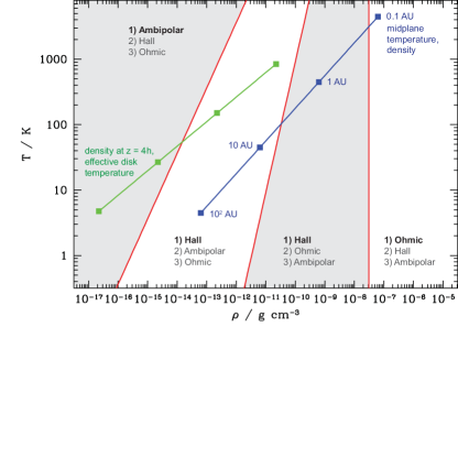
In reality, of course, Ohmic diffusion is not the only non-ideal process that can affect the evolution of the MRI. The full non-ideal MHD induction equation reads,
| (97) |
Here the current , and the third and fourth terms on the right-hand-side describe the Hall effect and ambipolar diffusion. The Hall effect depends upon the electron number density , while ambipolar diffusion depends upon the ion density and on the drag co-efficient describing the collisional coupling between ions and neutrals.
The absolute strength of the non-ideal effects depends upon the ionization state of the disk, and can be calculated with a chemical model. These models are generally complex, and subject to significant uncertainties arising, for example, from the unknown abundance of small dust grains that play an important role in recombination. Somewhat simpler is an estimate of the relative strengths of the different non-ideal terms, which follows from a dimensional analysis of equation (97) given assumptions as to the strength and structure of the magnetic field (Balbus & Terquem, 2001; Kunz & Balbus, 2004). Such an analysis is shown in Figure 16, which shows the estimated ordering of the importance of the different non-ideal terms as a function of the disk density and temperature. Ohmic diffusion is important at high densities (in the inner disk) whereas ambipolar diffusion dominates in disk regions where the density is very low (at large radii, and in the disk atmosphere). The Hall effect is most important at intermediate densities.
The nature of accretion that is driven by MHD processes in non-ideal disks has been studied with both local and global numerical simulations. Local or “shearing-box” simulations model a small co-rotating patch of disk with a linearized shear profile and radially periodic boundary conditions that are modified to account for the shear. Local simulations with reasonably realistic ionization models have been used to study protoplanetary accretion at radii between 1 and 100 AU:
-
•
In the outer disk (30-100 AU, and beyond) ambipolar diffusion is the dominant non-ideal effect. An approach similar to that used for Ohmic diffusion in §II.4.3 can be used to estimate when ambipolar diffusion damps the MRI, and the general expectations of such an estimate are borne out by simulations (Bai & Stone, 2011). In the absence of any net magnetic field ambipolar diffusion damps turbulence to such an extent that it is difficult to achieve accretion rates that match those observed much closer to the star (Simon et al., 2013a). Accretion rates that are of the right order of magnitude are only recovered if the disk is threaded with a weak net vertical field, with a ratio of mid-plane gas to magnetic pressure (in the vertical component) (Simon et al., 2013b). This result suggests that net fields—which are in any event an almost unavoidable consequence of star formation from magnetized molecular cloud cores—are also critical drivers of disk accretion.
-
•
In the inner disk (1-10 AU) the physics is more complex. Ohmic and ambipolar diffusion damp turbulence throughout most of the disk column, though in the presence of a net field accretion could still occur via angular momentum loss in a disk wind (Bai & Stone, 2013). Accretion in this region can also be driven by the Hall effect, as a result of the “Hall shear instability” (Kunz, 2008) which can amplify magnetic fields via a mechanism that is essentially independent of the usual MRI. The novel feature of the Hall effect is that it operates differently depending upon the sign of the net field relative to the angular momentum vector of the disk rotation. An aligned field leads to a substantial, largely laminar magnetic stress, while an anti-aligned field supports only very weak stress (Lesur, Kunz & Fromang, 2014; Bai, 2014).
Taken together the results of local simulations suggest that the strength and evolution of net disk fields are major players in disk evolution, and that the nature of accretion in the inner disk depends upon not just the strength but also the orientation of the field. Simulations by Simon et al. (2015) indicate that the angular momentum transport efficiency at 1 AU could differ by 1-2 orders of magnitude depending upon whether the net field in this region is aligned or anti-aligned to the rotation axis.
Local simulations are unsuitable tools for studies of disk winds, and so the fact that local models point to winds being important for protoplanetary disk accretion is more than a little concerning. Global simulations that include Ohmic and ambipolar diffusion have been reported by Gressel et al. (2015), while Béthune, Lesur & Ferreira (2017) present simulations including all three non-ideal effects. The global results are rather hard to summarize, but they confirm the likely importance of disk winds and suggest a weaker but still significant polarity dependence of angular momentum transport as a consequence the Hall effect. They also show the development of small-scale radial structure in the net field, via a process of self-organization that may have observable consequences for the distribution of dust within disks.
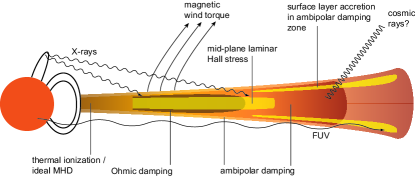
Figure 17 shows a schematic depiction of our “best guess” for what these non-ideal MHD simulation results imply for the global structure of protoplanetary disks. Three main regions are indicated. The innermost disk is hot enough to be thermally ionized, ideal MHD is a reasonable approximation, and the MRI results in turbulent transport of angular momentum. Further out turbulence is damped by a combination of Ohmic diffusion (near the mid-plane) and ambipolar diffusion (in the atmosphere). Angular momentum transport here may occur via largely laminar magnetic stresses, and there may also be angular momentum loss via disk winds. Finally, in the outer disk ambipolar diffusion damps the MRI strongly, with accretion occurring primarily in thin surface layers.
The paradigm of protoplanetary accretion described above, developed from theoretical considerations, is testable via several avenues. Furthest along are efforts to measure the turbulent broadening of molecular lines, which probe different regions of the vertical column depending upon their optical thickness (CO transitions, for example, are probes of the disk atmosphere, whereas HCO+ traces the mid-plane). To date, Flaherty et al. (2015) report upper limits of a few percent of the sound speed on turbulent broadening of CO lines in the HD 163296 system, while Teague et al. (2016) find results consistent with turbulence in the TW Hya disk at a level of 20-40 percent of the sound speed. These results may be compared to theoretical predictions for HD 163296 which imply turbulent velocities of at least tens of percent of the sound speed in the layer of the disk probed by CO (Simon et al., 2015b). There is an interesting conflict here between observations and theory, whose consequences remain to be understood.
II.4.5 Disk dispersal
Loss of the gaseous component of protoplanetary disks sets a time limit for the completion of gas giant formation, and will affect the environment for terrestrial planet formation as well. If only accretion is involved then the self-similar solution for a viscous disk (equation 68) predicts that the surface density and accretion rate decline as power-laws at late times, and hence that the transition between disk and diskless states should be very gradual. This will be modified if winds remove significant amounts of either mass or angular momentum from the disk. The best-developed models for dispersal focus on mass loss via thermal winds (photoevaporation), but mass or angular momentum loss in MHD flows may very well play a role as well if the disk retains magnetic flux throughout its lifetime (Armitage, Simon & Martin, 2013; Bai, 2016).
The original motivation for considering photoevaporarion came from HST observations of low mass stars exposed to the strong ionizing flux produced by massive stars in the core of the Orion Nebula’s Trapezium cluster O’Dell, Wen & Hu (1993). The images reveal tadpole-shaped nebulae surrounding young stars with circumstellar disks, which are interpreted as the signature of photoevaporation and escape of disk gas as a result of illumination by external ionizing radiation Johnstone, Hollenbach & Bally (1998). The physics underlying this process is relatively simple Bally & Scoville (1982); Shu, Johnstone & Hollenbach (1993); Hollenbach et al. (1994), and is closely related to the well-studied problem of Compton heated winds from accretion disks in Active Galactic Nuclei Begelman, McKee & Shields (1983). Extreme ultraviolet (EUV) photons with ionize and heat a surface layer of the disk, raising it to a temperature characteristic of an HII region. The sound speed in the photoionized gas is . Outside a critical radius , given by,
| (98) |
the sound speed in the hot gas exceeds the local Keplerian speed. The gas is then unbound, and flows away from the disk as a thermal wind. For a Solar mass star, as estimated by equation (98) is at 9 AU.
The same basic process can occur regardless of whether the EUV flux arises from an external source, such as a massive star in a cluster, or from the central star itself. In the typical star formation environment Lada & Lada (2003), however, most low mass stars receive too low a dose of EUV radiation from external sources to destroy their disks Adams et al. (2006). Photoevaporation due to radiation from the central star is therefore likely to be necessary for disk dispersal. In this regime, Hollenbach et al. (1994) derived an estimate for the mass loss rate due to photoevaporation,
| (99) |
where is the stellar ionizing flux. Most of the wind mass loss is predicted to originate close to , with a radial dependence of the mass loss given by . Numerical hydrodynamic simulations by Font et al. (2004) largely confirm this basic picture, although in detail it is found both that mass is lost for radii and that the integrated mass loss is a factor of a few smaller than that predicted by the above equation.
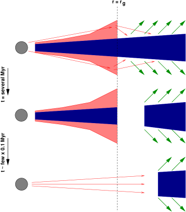
The combination of a photoevaporative wind and viscous disk evolution leads to rapid disk dispersal Clarke, Gendrin & Sotomayor (2001). Calculations by Alexander, Clarke & Pringle (2006) suggest a three-stage scenario depicted schematically in Figure 18,
-
•
Initially . The wind mass loss has negligible effect on the disk, which evolves in a similar way to an ordinary viscous model. The mass accretion rate and surface density gradually drop on the viscous time scale of the entire disk (determined at large radii), which is of the order of a Myr.
-
•
After a few Myr, the accretion rate drops sufficiently so that . The wind is then strong enough to dominate the disk surface density evolution near , opening up a gap in the disk and cutting off the inner disk from resupply by gas flowing in from the reservoir at larger radii. The inner disk then drains on to the star on its own (short) viscous time scale, which can be of the order of yr or less.
-
•
Once the inner disk has drained, the remaining gas in the outer disk is directly illuminated by UV radiation from the star (previously, the dominant flux was photons scattered on to the outer disk from a bound atmosphere at smaller radii). This radiation rapidly burns through the outer disk removing all remaining gas.
The primary source of uncertainty in these models is the origin and magnitude of the stellar ionizing flux. There are few constraints on for Solar mass T Tauri stars Alexander, Clarke & Pringle (2005), and essentially no information on any scaling with stellar mass.
The physics of the EUV-ionized gas flows described above is particularly easy to calculate. Qualitatively similar flows, however, can be driven by softer FUV radiation (), which suffices to dissociate H2 molecules and drives evaporative flow from the outer disk where the escape velocity is smaller. The detailed physics of such flows – which resemble photodissociation regions rather than HII regions – is harder to calculate because the temperature of the heated gas is determined by a balance between grain photoelectric heating and cooling by both atomic and molecular lines Adams et al. (2006); Gorti & Hollenbach (2009). Harder X-ray photons can also be important, and X-rays may in fact dominate the total photoevaporative mass loss rate for protoplanetary disks Ercolano, Clarke & Drake (2009). Alexander et al. (2014) provide a review of both the theory of these flows and some of the observational constraints on photoevaporation models.
II.5 The condensation sequence
In an actively accreting disk, there must be a temperature gradient in in order for energy to be transported from the dense midplane where it is probably liberated to the photosphere where it is radiated (note that for a thin disk with gradients in will dominate over radial gradients, which can consistently be ignored). A simple application of the theory of radiative transport in plane-parallel media Rybicki & Lightman (1979) allows us to derive the relation between the central disk temperature and the effective disk temperature .
To proceed, we define the optical depth to the disk midplane,
| (100) |
where is the Rosseland mean opacity and is the disk surface density. The vertical density profile of the disk is . If the vertical energy transport occurs via radiative diffusion (in some regions convection may also be important), then for the vertical energy flux is given by the equation of radiative diffusion,
| (101) |
Let us assume for simplicity that all the energy dissipation occurs at 111111In magnetized disks this is certainly not true, and both ideal (Miller & Stone, 2000) and non-ideal (Hirose & Turner, 2011) MHD simulations suggest that an interesting fraction of the dissipation may occur at low optical depths.. In that case is a constant with height. Integrating assuming that the opacity is a constant,
| (102) |
where for the final equality we have used the fact that for almost all of the disk gas lies below the photosphere. For large we expect that , and the equation simplifies to,
| (103) |
The implication of this result is that active disks with large optical depths are substantially hotter at the midplane than at the surface. For example, if to the thermal radiation emitted by the disk at some radius then . This is important since it is the central temperature that determines the sound speed that enters into the viscosity (equation 81), and it is also the central temperature that determines which ices or minerals can be present. Relatively modest levels of accretion can thus affect the thermal structure of the disk substantially.
For both terrestrial planet formation, and gas giant planet formation if it occurs via the core accretion mechanism, the evolution of the trace solid component of the disk is of great interest. The gas that forms the protoplanetary disk will contain interstellar dust grains made up of a mixture of silicates, graphite and polycyclic aromatic hydrocarbons (PAHs). In the interstellar medium, measurements of the wavelength dependence of extinction can be fit by assuming that the dust grains follow a power-law size distribution (Mathis, Rumpl & Nordsieck, 1977),
| (104) |
where is the grain size (assumed to be spherical) and the distribution extends from 0.005 m to about 1 m. This distribution is generally assumed to be the starting point for further evolution within the denser conditions prevailing within the disk. In the hottest, inner regions of the disk the central temperature can be high enough to destroy the grains (1000 K to 2000 K, depending on whether the grains are made of carbon or silicate). The resulting absence of dust very close to the star constitutes one of the main arguments against an in situ origin for hot Jupiters, but the dust destruction radius is sufficiently close in (normally substantially less than 1 AU) that it rarely impacts either terrestrial or, especially, giant planet formation. It is, however, important observationally, since once the dust is destroyed the remaining gas phase opacity is greatly reduced. There will therefore be an opacity “hole” in the inner disk even if gas is present there.
| Material | |
|---|---|
| 1680 K | Al2O3 |
| 1590 K | CaTiO3 |
| 1400 K | MgAl2O4 |
| 1350 K | Mg2SiO4, iron alloys |
| 370 K | Fe3O4 |
| 180 K | water ice |
| 130 K | NH3 H2O |
| 40 K – 80 K | methane, methane ices |
| 50 K | argon |
If the gas that makes up the protoplanetary disk has a known elemental composition (for example that of the Sun), then it is a well defined problem (for a chemist!) to calculate the most thermodynamically stable mix of chemical species at any given pressure and temperature. The abundance of different minerals and ices within the disk will follow this condensation sequence provided that there is sufficient time for chemical reactions to reach equilibrium. This may be a reasonable assumption in the hot inner disk but deviations will occur due to slow chemical reactions in the cool outer disk and radial drift of both gas and solids. The equilibrium mix depends more strongly on temperature than on pressure, so we can roughly map the condensation sequence into a predicted variation of disk composition with radius. Table II, adapted from Lodders (2003), lists characteristic temperatures below which different ices and minerals are predicted to be dominant. Of these, by far the most important is the temperature below which water ice can be present – this is 180 K at a pressure of 10-4 bar (though for the conditions in the protoplanetary disk, water ice requires moderately cooler conditions with ). For a Solar mix of elements, the surface density of condensable materials rises dramatically once water ice forms,
| (105) |
though the ratio depends upon still uncertain determinations of the exact Solar composition Lodders (2003). It is tempting – and extremely plausible – to associate changes in the efficiency or outcome of planet formation (in particular the division between terrestrial and gas giant planets in the Solar System) with the large change in the predicted surface density of solids that occurs at this radius.
The radius in the protoplanetary disk beyond which water ice can be present is called the snow line. In the Solar System, water-rich asteroids are found only in the outer asteroid belt Morbidelli et al. (2000), which suggests that the snow line in the Solar Nebula fell at around 3 AU. Passive protoplanetary disks are predicted to have snow lines at substantially smaller radii – in some cases interior to 1 AU – though accretion rates within the plausible range for Classical T Tauri disks suffice to push the snow line out to the inferred location of 3 AU Lecar et al. (2006); Garaud & Lin (2007).
III Planet Formation
The formation of planets from sub-micron size dust particles requires growth through at least 12 orders of magnitude in spatial scale. It is useful to consider different size regimes in which the interaction between the solid component and the gas is qualitatively distinct:
-
•
Dust – small particles ranging from sub-micron to cm in scale. These particles are well-coupled to the gas, but there can be slow drift either vertically or radially. Growth occurs through physical collisions leading to agglomeration.
-
•
“Rocks” – objects of meter scale. These particles have increasingly weak coupling to the gas, and so it can be useful to approximate their dynamics as being a combination of Keplerian orbits plus aerodynamic drag. Growth through this size regime is deduced to be rapid but the mechanism remains uncertain.
-
•
Planetesimals – bodies of km scale and above. Planetesimals are massive enough that their dynamics is largely decoupled from that of the gas. A population of bodies of this size is often considered as the initial condition for subsequent stage of planet formation, since the evolution of such a population is a well-posed N-body problem involving primarily purely gravitational forces (though for smaller planetesimals, questions regarding the bodies material strength can also be pertinent). In the classical scenario for planet formation we ignore dust and rocks once planetesimals have formed, but in fact aerodynamically assisted accretion of small bodies may play a substantial role in protoplanetary growth. This is “pebble accretion”.
-
•
Earth mass planets or progenitors of the giant planet cores. Once growing planets reach masses of the order of that of Earth, they again become coupled to the gas disk, though this time via gravitational rather than aerodynamic interactions. We will discuss this coupling later in the context of different regimes of planetary migration. For terrestrial planet formation it is possible that the formation of Earth mass bodies occurs after the gas disk has been dispersed (in which case this coupling is moot), but for growing giant planet cores it is inevitable that interaction will take place.
-
•
Planetary cores with masses of the order of . At around this mass, there is a transition from a quasi-hydrostatic core + envelope structure to a regime of rapid gas accretion.
Although it predates the discovery of extrasolar planetary systems, the review by Lissauer (1993) remains an excellent, readable summary of much of the physics that we will address in this section.
III.1 From dust to planetesimals
A spherical particle of radius , moving relative to the gas at velocity , experiences an aerodynamic drag force that opposes its motion,
| (106) |
where is the drag coefficient. The form of the drag coefficient depends upon the size of the particle compared to the mean free path of molecules in the gas Weidenschilling (1977b); Whipple (1972). For small particles (typically of cm size or less) for which,
| (107) |
the drag coefficient is,
| (108) |
where is the mean thermal velocity in the gas. This is called the Epstein regime of drag. For larger particles the Stokes drag law is valid. Defining the Reynolds number via,
| (109) |
where is the microscopic (molecular) viscosity in the gas, the drag coefficient can be expressed as a piecewise function,
| (110) |
We will apply these drag laws to consider both the vertical distribution and radial drift of small solid bodies within the gas disk.
III.1.1 Dust settling
Dust particles are strongly coupled to the gas via drag forces. For a particle of mass , the friction time scale is defined as,
| (111) |
It is the time scale on which drag will lead to order unity changes in the relative velocity between the particle and the gas. Writing the particle mass in terms of the material density , the friction time scale has a simple form in the Epstein regime,
| (112) |
Adopting conditions appropriate to 1 AU within the disk, , and we obtain . Small particles are thus very tightly coupled to the gas.
Consider a thin, vertically isothermal gas disk with surface density and scale height . The vertical density profile is,
| (113) |
To start with, let us ignore the effects of turbulence and assume that the disk is entirely quiescent. In this case the important forces acting on a particle at height above the midplane are the vertical component of gravity and gas drag, given by,
| (114) |
Given the strong coupling expected for dust particles terminal velocity will rapidly be attained, so we equate these to obtain the settling speed,
| (115) |
Settling is more rapid at higher (where the gas density is lower and the vertical component of gravity stronger), and for larger grains. For example, for micron sized dust particles at at 1 AU the settling velocity is and the settling time scale,
| (116) |
In the absence of turbulence, then, we expect micron sized dust particles to sediment out of the upper layers of the disk on a time scale that is short compared to the disk lifetime, while for particles with sizes the time scale is marginal.
Only the density in the equation for the settling time scale is a function of height. Inserting the expression for the vertical density profile the general expression for the settling time scale becomes,
| (117) |
The strong -dependence implies that dust will settle out of the upper regions of the disk rather rapidly in the absence of turbulence. This is of some interest since scattered light images of protoplanetary disks e.g. Burrows et al. (1996) are sensitive to dust well away from the midplane.
III.1.2 Settling in the presence of turbulence
The conditions necessary for turbulence to stir up the dust enough to oppose vertical settling can be estimated by comparing the settling time (equation 117) with the time scale on which diffusion will erase spatial gradients in the particle concentration. To diffuse vertically across a scale requires a time scale,
| (118) |
where is an anomalous (i.e. turbulent) diffusion co-efficient. Equating the settling and diffusion time scales at we find that turbulence will inhibit the formation of a particle layer with a thickness less than provided that,
| (119) |
This result is not terribly transparent. We can cast it into a more interesting form if we assume that the turbulence stirring up the particles is the same turbulence responsible for angular momentum transport within the disk. In that case it is plausible that the anomalous diffusion co-efficient has the same magnitude and scaling as the anomalous viscosity, which motivates us to write,
| (120) |
With this form for the minimum value of required for turbulence to oppose settling becomes,
| (121) |
which is roughly the ratio between the column density through a single solid particle and that of the whole gas disk. For small particles this critical value of is extremely small. If we take , and , for example, we obtain . This implies that small particles of dust will remain suspended throughout much of the vertical extent of the disk in the presence of turbulence with any plausible strength. For larger particles the result is different. If we consider particles of radius 1 mm – a size that we know from observations is present within disks – we find that the critical value of . This value is comparable to most large scale estimates of for protoplanetary disks. Particles of this size and above will therefore not have the same vertical distribution as the gas in the disk.
To proceed more formally we can consider the solid particles as a separate fluid that is subject to the competing influence of settling and turbulent diffusion. If the “dust” fluid with density can be treated as a trace species within the disk (i.e. that ) then it evolves according to an advection-diffusion equation of the form (Fromang & Papaloizou, 2006; Dubrulle, Morfill & Sterzik, 1995),
| (122) |
Simple steady-state solutions to this equation can be found in the case where the dust layer is thin enough that the gas density varies little across the dust scale height. In that limit the dimensionless friction time is independent of and we obtain,
| (123) |
where , the scale height describing the vertical distribution of the particle concentration , is,
| (124) |
If, as previously, we assume that , we can write a compact expression for the ratio of the concentration scale height to the usual gas scale height,
| (125) |
The condition for solid particles to become strongly concentrated toward the disk midplane is then that the dimensionless friction time is substantially greater than . For any reasonable value of this implies that substantial particle growth is required before settling takes place.
Our discussion of dust settling in the presence of turbulence sweeps a number of tricky issues under the carpet. More careful treatments need to consider:
-
•
Whether plausible sources of disk turbulence really generate an effective turbulent diffusivity that is related to the effective turbulent viscosity. There has been a great deal of work on this issue over the years – a good modern starting point is Zhu, Stone & Bai (2015).
-
•
The relationship between the effective diffusivity of the gas and that of particles aerodynamically coupled to it. This is non-trivial once particles become large enough that (Youdin & Lithwick, 2007).
III.1.3 Settling with coagulation
In addition to being affected by turbulence, settling is also coupled to coagulation and particle growth. The settling velocity increases with the particle size, so coagulation hastens the collapse of the dust toward the disk midplane.
To estimate how fast particles could grow during sedimentation we appeal to a simple single particle growth model (Safronov, 1969; Dullemond & Dominik, 2005). Imagine that a single “large” particle, of radius and mass , is settling toward the disk midplane at velocity through a background of much smaller solid particles. By virtue of their small size, the settling of the small particles can be neglected. If every collision leads to coagulation, the large particle grows in mass at a rate that reflects the amount of solid material in the volume swept out by its geometric cross-section,
| (126) |
where is the dust to gas ratio in the disk. Substituting for the settling velocity one finds,
| (127) |
Since this Equation cannot generally be integrated immediately121212Note however that if the particle grows rapidly (i.e. more rapidly than it sediments) then the form of the equation implies exponential growth of with time., but rather must be solved in concert with the equation for the height of the particle above the midplane,
| (128) |
Solutions to these equations provide a very simple model for particle growth and sedimentation in a non-turbulent disk.

Figure 19 shows solutions to equations (127) and (128) for initial particle sizes of 0.01 m, 0.1 m and 1 m. The particles settle from an initial height through a disk whose parameters are chosen to be roughly appropriate to a (laminar) Solar Nebula model at 1 AU from the Sun. Both particle growth and vertical settling are extremely rapid. With the inclusion of coagulation, particles settle to the disk midplane on a time scale of the order of yr – more than two orders of magnitude faster than the equivalent time scale in the absence of particle growth. By the time that the particles reach the midplane they have grown to a final size of a few mm, irrespective of their initial radius.
The single particle model described above is very simple, both in its neglect of turbulence and because it assumes that the only reason that particle-particle collisions occur is because the particles have different vertical settling velocities. Other drivers of collisions include Brownian motion, turbulence, and differential radial velocities. The basic result, however, is confirmed by more sophisticated models (Dullemond & Dominik, 2005), which show that if collisions lead to particle adhesion growth from sub-micron scales up to small macroscopic scales (of the order of a mm) occurs rapidly. There are no time scale problems involved with the very earliest phases of particle growth. Indeed, what is more problematic is to understand how the population of small grains – which are unquestionably present given the IR excesses characteristic of Classical T Tauri star – survive to late times. The likely solution to this quandary involves the inclusion of particle fragmentation in sufficiently energetic collisions, which allows a broad distribution of particle sizes to survive out to late times. Fragmentation is not likely given collisions at relative velocities of the order of a cm s-1 – values typical of settling for micron-sized particles – but becomes more probable for collisions at velocities of a m s-1 or higher.
III.1.4 Radial drift of particles
Previously we showed (equation 54) that the azimuthal velocity of gas within a geometrically thin disk is close to the Keplerian velocity. That it is not identical, however, turns out to have important consequences for the evolution of small solid bodies within the disk Weidenschilling (1977b). We can distinguish two regimes,
-
•
Small particles () are well-coupled to the gas. To a first approximation we can imagine that they orbit with the gas velocity. Since they don’t experience the same radial pressure gradient as the gas, however, this means that they feel a net inward force and drift inward at their radial terminal velocity.
-
•
Rocks () are less strongly coupled to the gas. To a first approximation we can imagine that they orbit with the Keplerian velocity. This is faster than the gas velocity, so the rocks see a headwind that saps their angular momentum and causes them to spiral in toward the star.
To quantify these effects, we first compute the magnitude of the deviation between the gas and Keplerian orbital velocities. Starting from the radial component of the momentum equation,
| (129) |
we write the variation of the midplane pressure with radius as a power-law near radius ,
| (130) |
where . Substituting, we find,
| (131) |
where
| (132) |
Typically is positive (i.e. the pressure decreases outward), so the gas orbits slightly slower than the local Keplerian velocity. For example, for a disk of constant and surface density profile we have and,
| (133) |
The fractional difference between the gas and Keplerian velocities is small indeed! However, at 1 AU even this small fractional difference amounts to a relative velocity of the order of 100 ms-1. Large rocks will then experience a substantial, albeit subsonic, headwind.
The effect of the drag force on the dynamics of particles of arbitrary sizes has been calculated by Weidenschilling (1977b). Here, we adopt the approach of Takeuchi & Lin (2002) and proceed by considering the radial and azimuthal equations of motion for the particle131313Although this calculation is straightforward, it’s easy to confuse the three different azimuthal velocities that are involved – that of the particle, that of the gas, and the Kepler speed. Be careful!,
| (134) |
We simplify the azimuthal equation by noting that the specific angular momentum always remains close to Keplerian (i.e. the particle spirals in through a succession of almost circular, almost Keplerian orbits),
| (135) |
This yields,
| (136) |
Turning now to the radial equation, we substitute for using equation (131). Retaining only the lowest order terms,
| (137) |
The term is negligible, and for simplicity we also assume that , which will be true for those particles experiencing the most rapid orbital decay. Eliminating between equations (136) and (137) we obtain,
| (138) |
This result can be cast into a more intuitive form by defining a dimensionless stopping time,
| (139) |
in terms of which the particle radial velocity is,
| (140) |
The peak radial velocity is attained when (i.e. when the friction time scale equals ), and equals independent of the disk properties.

Figure 20 plots as a function of the dimensionless stopping time for a fiducial disk with . Using equations (108) and (110), one can associate a particular with a unique particle size given known conditions in the protoplanetary disk. Generically, one finds that at radii of a few AU the peak inspiral rate is attained for particles with size of the order of 10 cm to a few m. The minimum inspiral time scale at a given orbital radius depends only on – at 1 AU it is of the order of 100 yr. The inescapable conclusion is that the radial drift time scale disk lifetime for meter-scale bodies in the protoplanetary disk.
The above analysis assumes that the density of solid particles is low enough (compared to the gas density) that there is no back-reaction of the solids on the gas. In some important circumstances (particularly when considering models for planetesimal formation) this criterion will be violated. Nakagawa, Sekiya & Hayashi (1986) have calculated models of settling and radial drift that are valid in the more general case where the solid and gas phases can have comparable densities.
As we noted earlier, the fact that most of the heavy elements in the Solar System are found in the Sun means that we can tolerate some loss of planetary raw material during planet formation. However, radial drift time scales as short as 100 yr would clearly lead to a catastrophic loss of mass into the star unless, in fact, growth through the meter-scale size regime is very fast. The most important conclusion from this analysis is, therefore, that planetesimal formation must be a rapid process. This is a robust inference since it derives directly from the unavoidable existence of a velocity differential between the gas disk and solid bodies orbiting within it.
The radial drift velocities given by equation (140) imply significant radial migration over the lifetime of the disk – not just for particles at the most vulnerable meter-scale size range but also for substantially smaller and larger bodies. This means that we should expect substantial changes in the local ratio of solids to gas as a function of time and radius in the disk Takeuchi, Clarke & Lin (2005). Under some circumstances, radial drift may allow solids to pileup within the inner disk, potentially improving the chances of forming planetesimals there Youdin & Chiang (2004).
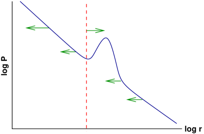
Radial drift can be slowed or locally reversed if the gas disk has a non-monotonic radial pressure profile. The inward motion of solid bodies embedded within the disk occurs as a consequence of a gas pressure gradient that leads to sub-Keplerian gas orbital velocities. In general, radial drift drives particles toward pressure maxima, so in a disk where the mid-plane pressure declines smoothly the motion is typically inward. If, on the other hand, it were possible to create local pressure maxima these would also act as sites where solids concentrate. This possibility was recognized in a prescient paper by Whipple (1972), whose Figure 1 is more or less reproduced here as Figure 21. If the perturbation to the pressure occurs on a scale , then to obtain a maximum we require that the local pressure gradient exceed the global gradient . The time scale to concentrate solids locally is then faster than the global inspiral time by a factor .
Several physical processes can create pressure maxima. Persistent local pressure maxima could form in a disk at particular locations (for example, at the inner edge of dead zones), while transient maxima could occur due to the large-scale effects of disk turbulence. Rice et al. (2004) and Durisen et al. (2005) discussed how self-gravitating turbulence might concentrate particles within spiral arms or axisymmetric gas rings. Johansen, Youdin & Klahr (2009b) showed that “zonal flows”—axisymmetric local perturbations to the pressure that are maintained by variations in —could form within MRI turbulent disks. The edges of gaps carved by massive planets are another obvious location where a pressure maxima may be expected.
III.1.5 Planetesimal formation via coagulation
The growth of micron-sized dust particles up to small macroscopic dimensions (of the order of a mm) is driven by pairwise collisions that lead to sticking and particle growth. (Simultaneously, high velocity impacts may lead to fragmentation.) The most economical hypothesis for planetesimal formation is that the same process continues uninterrupted up to the planetesimal size scale (for an early calculation, see e.g. Weidenschilling, 1980). A coagulation model for planetesimal formation, however, faces two independent challenges. First, the material properties of colliding bodies with a realistic velocity distribution must permit growth (rather than bouncing or fragmentation) across the full range of sizes between dust particles and planetesimals. Second, the rate of growth must be high enough to form planetesimals before the material is lost into the star via aerodynamic drift. These constraints are not easily satisfied (or summarized), but neither are they obviously insurmountable.
The outcome of collisions between micron to cm-sized bodies can be studied experimentally, ideally under low-pressure microgravity conditions. Good introductions to the extensive literature on experimental results are given by Blum & Wurm (2008), Güttler et al. (2010) and Testi et al. (2014). The bulk of the experimental work has been performed using silicate particles and aggregates, representative of materials found interior to the snow line. The most basic result is the critical velocity below which individual grains stick together. For silicate monomers this velocity is about 1 (Poppe, Blum & Henning, 2000). For similarly sized water ice monomers the velocity is approximately 10 (Gundlach & Blum, 2015). This order of magnitude difference presages the likelihood of differences in particle growth outcomes interior to and outside the water snow line.
Going beyond monomers, it is generally assumed that the colliding bodies are aggregates made up these smaller sub-units. The porosity of the aggregates represents an extra dimension that must be taken into account in modeling growth. A porous body can dissipate energy on collision through rearrangement of its structures (and hence can be “stronger” in some sense than a single particle), but can also be compactified by the action of multiple collisions. Theoretical models suggest that aggregates growing outside the snow line can, in some situations, be extremely porous, with internal densities as low as (Okuzumi et al., 2012).
Models for particle growth need to account consistently for how the size distribution evolves given the predicted collision speeds between particles (Weidenschilling & Cuzzi, 1993; Ormel & Cuzzi, 2007), the experimentally measured or theoretically predicted collision outcomes, and the local change in solid density due to radial drift. It’s a difficult problem whose solution is uncertain. Generally it appears that:
-
•
There are no material barriers preventing monomers from growing into at least mm-sized particles anywhere in the disk. The size distribution of particles in the range between and is likely set by a balance of coagulation and fragmentation processes (Birnstiel, Ormel & Dullemond, 2011).
-
•
Interior to the snow line, the onset of bouncing creates a barrier to growth at around mm or cm sizes (Zsom et al., 2010). Growth likely continues beyond these sizes, but is more severely limited by fragmentation and is not fast enough to form planetesimals in the presence of radial drift.
-
•
Outside the snow line, growth to larger sizes is in principle allowed because icy particles stick at higher velocities and are more resistant to fragmentation (which may not occur until collision velocities reach several tens of meters per second). Growth may be limited by radial drift itself, leading to a “drift-limited growth” scenario in which the particle size as a function of radius is determined by the condition that that the growth time roughly equals the drift time (Birnstiel, Klahr & Ercolano, 2012). Growth to larger sizes is possible if the disk structure supports persistent or transient particle traps that slow radial drift (Pinilla et al., 2012).
- •
Based upon these results most workers infer that a planetesimal formation mechanism distinct from simple collisional growth is needed to explain how planetesimals can form across a broad range of radii both interior to and outside the snow line.
III.1.6 The Goldreich-Ward mechanism
The alternate hypothesis for planetesimal formation holds that planetesimals form from gravitational fragmentation of dense clumps of particles. In its simplest form, particles might settle vertically so strongly that a dense sub-disk of solids at the mid-plane becomes vulnerable to collapse (Goldreich & Ward, 1973)141414Similar considerations are discussed in Safronov (1969), who in turn quotes earlier work by Gurevich & Lebedinskii from as early as 1950.. As we will discuss this specific model does not work, because it turns out to be very difficult to settle a layer of small dust particles to densities high enough for gravitational instability. Nonetheless the basic idea remains attractive since it forms planetesimals while entirely bypassing the size scales that are most vulnerable to radial drift, and it useful to discuss the original idea before considering contemporary theories for planetesimal formation that likewise invoke collective instabilities followed by fragmentation.
The basic idea of the Goldreich-Ward (1973) mechanism for planetesimal formation is that vertical settling and radial drift results in the formation of a dense dust sub-disk within which the solid density exceeds the local gas density (this obviously requires a very thin sub-disk if the local ratio of gas to dust surface density is comparable to the fiducial global value of 100). The solid sub-disk then becomes gravitationally unstable, and fragments into bound clumps of solid particles that subsequently dissipate energy via physical collisions and collapse to form planetesimals.
Gravitational instability requires that the disk be massive (high surface density) and / or dynamically cold (low velocity dispersion). The classic analysis of the conditions for gravitational instability is that of Toomre (1964). Here, we consider the stability of a rotating fluid sheet – this is somewhat easier than the collisionless calculation, gives the same answer to a small numerical factor when the gas sound speed is identified with the particle velocity dispersion, and carries over to the instability of a gas disk that we will discuss later. The simplest system to analyze is that of a uniformly rotating sheet – in what follows I follow the notation and approach of Binney & Tremaine (1987).
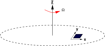
The setup for the calculation is as shown in Figure 22. We consider a sheet of negligible thickness in the plane, with constant surface density and angular velocity . Our aim is to calculate the stability of the sheet to in-plane perturbations. Working in a frame that corotates with the (unperturbed) angular velocity , the fluid equations are,
| (141) | |||||
| (142) | |||||
where the momentum equation picks up terms for the Coriolis and centrifugal forces in the rotating frame. These equations apply in the plane only. The gravitational potential is given by the Poisson equation,
| (143) |
which describes in all space. In these equations, is the velocity in the rotating frame, is the surface density, and is the vertically integrated pressure. The sound speed is defined via,
| (144) |
In the unperturbed state, , , and . Substituting these values into the momentum equation yields .
We now consider perturbations to the surface density, velocity, pressure and potential,
| (145) |
where it is assumed that etc. Substituting these expressions into the fluid equations, and retaining only those terms that are linear in the perturbed quantities, we find,
| (146) | |||||
| (147) | |||||
| (148) |
where we have made use of the fact that since is only a function of , . Note that these equations only involve temporal or spatial derivatives of the perturbed quantities. Since the equations are (by construction) linear, the evolution of an arbitrary perturbation can be decomposed into fourier modes. Assuming a wavevector that is parallel to , we therefore write the perturbations in the form,
| (149) | |||||
| (150) | |||||
| (151) |
where the final expression describes the potential perturbations in the plane only. Substitution of these expressions into the perturbation equations will reduce them to algebraic expressions, which can be combined to yield the dispersion relation for the system.
First though, we simplify the system by noting that perturbations in are the source of perturbations in . We can therefore write in terms of . To do this, let the general form for (i.e. not just at ) be,
| (152) |
where is some function that needs to be determined. Requiring that for , we find,
| (153) |
which has a general solution , with and arbitrary constants. Since must remain finite as , the general form of is,
| (154) |
This is valid throughout all space.
To determine , we integrate the Poisson equation vertically between and ,
| (155) |
Mathematically this requires a bit of care, since the integrand on the left hand side is zero everywhere except at . However, noting that and are continuous at , while is not, we obtain,
| (156) |
Taking the limit as ,
| (157) |
and,
| (158) |
We are now in a position to substitute , and into the remaining equations (continuity plus the and components of the momentum equation). The resulting algebraic equations are,
| (159) | |||||
| (160) |
We seek a dispersion relation i.e. a formula for the growth rate of modes of different scale . Eliminating and in turn, we obtain,
| (161) |
This is the dispersion relation for a uniformly rotating thin sheet. The scale-dependence of the different terms is shown graphically in Figure 23.
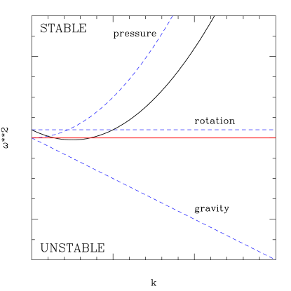
Looking back to the form of the perturbations, we note that the sheet is:
-
•
STABLE if , since in this case is real and the perturbations are oscillatory.
-
•
UNSTABLE if , for which case is imaginary and perturbations grow exponentially.
The rotational term () is stabilizing at all scales, while the pressure term () has a strong stabilizing influence at large (i.e. small spatial scales). Self-gravity, represented by the term, has a negative contribution to and so destabilizes the sheet.
The condition for marginal stability is that at all spatial scales. The most unstable scale can be found by setting , which yields,
| (162) |
The sheet is marginally stable when , which gives the stability condition as,
| (163) |
This analysis can be extended in several ways – for example to include differential rotation or global rather than local stability. A generic way of expressing the results of such calculations is to define the Toomre parameter,
| (164) |
In terms of , a disk is unstable151515For a differentially rotating disk, it is easy to verify that stability depends upon the parameter combination via a time scale argument. First derive the time scale for shear to separate two points that are initially apart, and equate this to the collapse time scale under gravity to find the maximum scale on which collapse can occur without being affected by shear. Taking the ratio of this scale to the Jeans scale (the smallest scale on which collapse can occur without being inhibited by pressure gradients) yields the correct functional form of . to its own self-gravity if , and stable if . Typically – for the specific system we have investigated it would be .
We have derived the stability of a fluid disk in uniform rotation. Differential rotation and global effects alter the value of , but do not fundamentally change the result. For a collisionless disk (e.g. one made of stars or small solid particles) a comparable result applies if we replace the sound speed by the one-dimensional velocity dispersion .
The most unstable wavelength is,
| (165) |
Comparing this to the scale height of the disk , we find that at marginal stability,
| (166) |
i.e. the instability afflicts small-ish spatial scales within the disk.
Let us apply this analysis to the problem of planetesimal formation. If we ignore radial drift, then at 1 AU , or about 10 g cm-2 for a minimum mass Solar Nebula model (note that a gas to dust ratio of 100 is a commonly used approximation in protoplanetary disk theory). Setting , and taking , we find that instability requires a critical velocity dispersion in the solid component,
| (167) |
Since the gas sound speed at this radius is of the order of , and the scale heights of the gas and particle disks are respectively proportional to and , we see that an extremely thin disk is required before instability will set in!
If instability occurs, the most unstable wavelength is predicted to be,
| (168) |
The mass within an unstable patch is then,
| (169) |
which would correspond to a spherical body of size,
| (170) |
for a material density of . The collapse time scale at distance from mass ,
| (171) |
is very short – less than a year for the parameters adopted above. Even if we allow for the fact that angular momentum will preclude a prompt collapse, the derived time scale for planetesimal formation via gravitational instability remains extremely short – perhaps of the order of 103 yr Goldreich & Ward (1973).
Formation of planetesimals via the Goldreich-Ward mechanism has several attractive features, most notably the short time scale and complete bypass of the size regime most vulnerable to radial drift. However in its simplest form, the mechanism fails to work. The problem lies in the fact that even in an intrinsically non-turbulent gas disk, the formation of a dense solid sub-disk leads to self-generated turbulence and associated vertical stirring prior to gravitational instability. As noted above, for gravitational instability to operate we require a thin sub-disk in which, for our choice of parameters,
| (172) |
Within this midplane layer, the volume density of solids would exceed the density of gas by a factor of the order of 100 – i.e. the extreme thinness of the solid disk inverts the normal gas to dust ratio which favors gas by the same factor. Since the gas and dust are well coupled for small particle sizes, within the sub-disk (where the solid component dominates) we expect both the gas and the dust to orbit at the natural velocity for the solid component, which is the Kepler velocity. The gas just above the layer, on the other hand, will rotate slower due to the radial gas pressure gradient. There will therefore be a velocity gradient in the direction that is of the order of . This shear will be Kelvin-Helmholtz unstable, leading to turbulence that prevents the layer ever getting thin enough to fragment into planetesimals Cuzzi, Dobrovolskis & Champney (1993). The condition for Kelvin-Helmholtz instabilities to develop Sekiya (1998); Youdin & Shu (2002) is that the Richardson number, which measures the competition between vertical shear and buoyancy, is , where,
| (173) |
and , the Brunt Väisälä frequency, is defined as,
| (174) |
The standard stability analysis obtains a critical Richardson number , but both analytic calculations including the effect of Coriolis forces, and numerical simulations, favor a larger value of around unity Gomez & Ostriker (2005); Johansen, Henning & Klahr (2006).
III.1.7 Streaming instabilities
Although it is very hard to settle a particle layer to the point where it becomes gravitational unstable, coagulation plus settling can plausibly lead to a mid-plane layer in which the local particle density is comparable to that of the gas . Current interest in gravitational instability as a mechanism for planetesimal formation is based upon the realization that the weaker condition suffices to trigger non-gravitational clumping of particles via the streaming instability, that can be strong enough to form clumps that will subsequently collapse under self-gravity.
The term “streaming instability” is used generically to describe instability in aerodynamically coupled mixtures of particles and gas in Keplerian disks. The original analysis by Youdin & Goodman (2005) considered a vertically unstratified system in which an incompressible gas interacts with a compressible particle “fluid” via two-way aerodynamic forces161616Particle clustering in turbulence also occurs in the “passive” limit where the aerodynamic back reaction on the gas is neglected. In this regime, particles concentrate in the regions between vortices. This type of aerodynamic clustering may have interesting consequences for protoplanetary disks (Cuzzi, Hogan & Shariff, 2008; Pan et al., 2011), but the natural scale is much smaller (of the order of the viscous scale in the turbulence) and the process is entirely distinct from the streaming instability.. This system is described by a pair of continuity and momentum equations representing the two fluids,
| (175) |
(The notation here ought to be self-explanatory.) The above equations are not a full description of the physical system found in protoplanetary disks. Vertical stratification is neglected, together with the effect of intrinsic turbulence which might loosely be supposed to lead to an effective diffusivity for the particles. Taking the gas to be incompressible and treating the particles as a fluid (with, necessarily, a single-valued velocity field at each point) are good approximations, but approximations nonetheless.
The equilibrium state of steady radial drift defined by the above equations is the Nakagawa-Sekiya-Hayashi (NSH) equilibrium mentioned earlier (Nakagawa, Sekiya & Hayashi, 1986). Youdin & Goodman (2005) showed that the NSH equilibrium is linearly unstable for a broad range of system parameters, of which the important ones are the local solid to gas ratio, the dimensionless stopping time of the particles, and the amount of pressure support in the gas. The simplest unstable modes are axisymmetric, typically of small scale (substantially smaller than ), and have growth rates that can be as large as but which are often much smaller. The linear instability does not have any known explanation that is particularly compelling or intuitive.
Numerical simulations have established that the streaming instability provides a pathway to forming dense clumps that can collapse gravitationally to form planetesimals (Johansen et al., 2007), though the pre-requisite particle size and local metallicity are not trivially satisfied. Work by Carrera, Johansen & Davies (2015) and Yang, Johansen & Carrera (2017) shows that the non-linear evolution of the streaming instability leads to strong clumping that would precipitate rapid planetesimal formation in a U-shaped region of local metallicity / stopping time space spanning . The lowest required metallicity—which is still super-Solar (Johansen, Youdin & Mac Low, 2009)—occurs for , which corresponds to particles larger than those that obviously form from coagulation in the inner disk. Smaller values of , which lead to strong clumping only for metallicities of , match up better with expected initial particle sizes. It appears plausible that planetesimal formation occurs, albeit at a slower rate, for local solid to gas ratios modestly lower than the currently established thresholds.
Once collapse of streaming-initiated over-densities occurs the outcome is a population of planetesimals. The initial mass function of the resultant planetesimals can be fit with a power-law that is cut-off above some characteristic mass. A recent determination by Simon et al. (2016) obtains a differential mass function,
| (176) |
with . Results by Schäfer, Yang & Johansen (2017) are consistent. This is a mass function in which the largest bodies in the population have most of the mass.
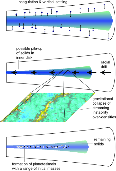
Figure 24 illustrates how the various processes that we have discussed—coagulation, vertical settling, radial drift, and the streaming instability—might conspire together to lead to planetesimal formation. It is not obvious what radial profile of planetesimal surface density ought to result, though barring some remarkable fluke it will not be the simple power-law envisaged in the Minimum Mass Solar Nebula model. There has been some discussion of how the hypothesis that the streaming instability forms planetesimals could be tested, either in the asteroid belt (Morbidelli et al., 2009) or in the Kuiper Belt (Nesvorný, Youdin & Richardson, 2010), but more work is needed before drawing strong conclusions.
Other flavors of particle clustering in turbulence may also be important. Attaining the relatively high local dust to gas ratios needed to trigger the streaming instability may be aided and abetted by local pressure maxima in zonal flows (Johansen, Youdin & Klahr, 2009b; Simon & Armitage, 2014) or vortices (Barge & Sommeria, 1995), which may be formed at the edges of dead zones (Lyra et al., 2009). The loss of gas (Throop & Bally, 2005) and formation of an inner hole via photoevaporative disk dispersal (Alexander & Armitage, 2007) could also enhance , potentially triggering a late episode of planetesimal formation.
III.2 Growth beyond planetesimals
Once planetesimals have formed the gas in the disk will continue to influence their dynamics through two diametrically opposed effects. Residual aerodynamic interactions will act to damp planetesimal eccentricity and inclination, while surface density fluctuations produced by turbulence will exert fluctuating gravitational forces that excite eccentricity (Laughlin, Steinacker & Adams, 2004; Nelson, 2005; Okuzumi & Ormel, 2013). These effects are significant, but overall further dynamical interaction between the solid and gaseous components of the disk is limited until bodies with sizes form that are large enough to have a gravitational coupling to the gas. We will discuss the impact of gravitational coupling (“migration”) later in the context of the early evolution of planetary systems.
How do planetesimals grow to form planetary embryos, planets and giant planet cores? We will start by discussing the physics of the classical model for planet formation, in which the dominant dynamics is mutual gravitational interactions between the bodies and growth occurs from planetesimal-planetesimal and eventually planetesimal-protoplanet collisions. This is a well-posed problem that is usually studied using a combination of statistical and N-body methods. Later, we will describe a popular modern variant in which the dynamics remains largely gravitational, but where growth occurs due to the aerodynamically assisted accretion of small particles (“pebbles”) that failed to form planetesimals.
III.2.1 Gravitational focusing
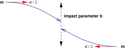
For sufficiently small bodies, the effects of gravity can be ignored for the purposes of determining whether they will physically collide. A massive planet, on the other hand, can gravitationally focus other bodies toward it, and as a result has a collision cross section that is much larger than its physical cross section.
To evaluate the magnitude of this gravitational focusing, consider two bodies of mass , moving on a trajectory with impact parameter , as shown in Figure 25. The relative velocity at infinity is . At closest approach, the bodies have separation and velocity . Equating energy in the initial (widely separated) and final (closest approach) states we have,
| (177) |
Noting that there is no radial component to the velocity at the point of closest approach, angular momentum conservation gives,
| (178) |
If the sum of the physical radii of the bodies is , then for there will be a physical collision, while larger will result in a harmless flyby171717This is true for solid bodies – for giant planets or stars tidal effects can lead to significant dissipation of energy even when Fabian, Pringle & Rees (1975).. The largest value of the impact parameter that will lead to a physical collision is thus,
| (179) |
which can be expressed in terms of the escape velocity from the point of contact, as,
| (180) |
The cross section for collisions is then,
| (181) |
where the term in brackets represents the enhancement to the physical cross section due to gravitational focusing. Clearly a planet growing in a “cold” planetesimal disk for which will grow much more rapidly as a consequence of gravitational focusing. As a consequence, determining the velocity dispersion of bodies of different masses during the planet formation process is extremely important.
III.2.2 Growth versus fragmentation
When two initially solid bodies physically collide the outcome can be divided broadly into three categories:
-
•
Accretion. All or most of the mass of the impactor becomes part of the mass of the final body, which remains solid. Small fragments may be ejected, but overall there is net growth.
-
•
Shattering. The impact breaks up the target body into a number of pieces, but these pieces remain part of a single body (perhaps after reaccumulating gravitationally). The structure of the shattered object resembles that of a rubble pile.
-
•
Dispersal. The impact fragments the target into two or more pieces that do not remain bound.
To delineate the boundaries between these regimes quantitatively, we consider an impactor of mass colliding with a larger body of mass at velocity . We define the specific energy of the impact via,
| (182) |
and postulate that this parameter largely controls the result. The thresholds for the various collision outcomes can then be expressed in terms of . Conventionally, we define the threshold for catastrophic disruption as the minimum specific energy needed to disperse the target in two or more pieces, with the largest one having a mass . Similarly is the threshold for shattering the body. More work is required to disperse a body than to shatter it, so evidently . It is worth keeping in mind that in detail the outcome of a particular collision will depend upon many factors, including the mass ratio between the target and the impactor, the angle of impact, and the shape and rotation rate of the bodies involved. Quoted values of are often averaged over impact angles, but even when this is done the parameterization of collision outcomes in terms of is only an approximation.
The estimated values of for a target of a particular size vary by more than an order of magnitude depending upon the composition of the body, which can broadly be categorized into solid or shattered rock, and solid or porous ice. For any particular type of body, however, two distinct regimes can be identified:
-
•
Strength dominated regime. The ability of small bodies to withstand impact without being disrupted depends upon the material strength of the object. In general, the material strength of bodies declines with increasing size, owing to the greater prevalence of defects that lead to cracks. In the strength dominated regime decreases with increasing size.
-
•
Gravity dominated regime. Large bodies are held together primarily by gravitational forces. In this regime must at the very least exceed the specific binding energy of the target, which scales with mass and radius as . In practice it requires a great deal more than this minimum amount of energy to disrupt the target – so is not a good estimate of – but nonetheless does increase with increasing size.
Although the transition between these regimes is reasonably sharp there is some influence of the material properties (in particular the shear strength) on the catastrophic disruption threshold for smaller bodies within the gravity dominated regime.
Values of and can be determined experimentally for small targets (Arakawa, Leliwa-Kopystynski & Maeno, 2002). Experiments are not possible in the gravity dominated regime, but can be estimated theoretically using numerical hydrodynamics (Benz & Asphaug, 1999; Leinhardt & Stewart, 2009) or (for rubble piles) rigid body dynamics simulations (Leinhardt & Richardson, 2002; Korycansky & Asphaug, 2006). The simplest parameterization of the numerical results is as a broken power law that includes terms representing the strength and gravity regimes,
| (183) |
Often (but not always) is averaged over impact geometry, and , , and are all constants whose values are derived by fitting to the results of numerical simulations.
| / | / | / | |||
|---|---|---|---|---|---|
| km s-1 | erg g-1 | erg cm3 g-2 | |||
| Ice (weak) | 1.0 | 0.09 | -0.40 | 1.30 | |
| Ice (strong) | 0.5 | 2.1 | -0.45 | 1.19 | |
| Ice (strong) | 3.0 | 1.2 | -0.39 | 1.26 | |
| Basalt (strong) | 3.0 | 0.3 | -0.38 | 1.36 | |
| Basalt (strong) | 5.0 | 0.5 | -0.36 | 1.36 |

Benz & Asphaug (1999) and Leinhardt & Stewart (2009) determined the values of the fitting parameters in equation (183) from the results of an ensemble of simulations of impacts into icy or rocky targets. Their results are given in Table 3 and plotted as a function of target size in Figure 26. One observes immediately that the results for a particular target material vary with the impact velocity, and hence that is not the sole determinant of the outcome of collisions. There is, however, a clear transition between the strength and gravity dominated regimes, with the weakest bodies being those whose size is comparable to the cross-over point. The most vulnerable bodies are generally those with radii in the 100 m to 1 km range. Just how vulnerable such bodies are to catastrophic disruption depends sensitively on their make-up, and it would be unwise to place too much trust in precise numbers. As a rough guide, however, the weakest icy bodies have minimum , while the strongest conceivable planetesimals (unfractured rocky bodies) have minimum .
As a reality check, we may note that asteroids in the main belt with would be expected to collide today with typical velocities of the order of 2 km s-1. For a mass ratio the specific energy of the collision is then around , which from Figure 26 is sufficient to destroy even quite large solid bodies with . This is consistent with the observation of asteroid families, and the interpretation of such families as collisional debris. Evidently the random velocities that characterize collisions must have been much smaller during the epoch of planet formation if we are to successfully build large planets out of initially km-scale planetesimals.
III.2.3 Shear versus dispersion dominated encounters
A more subtle distinction that nevertheless plays a crucial role in planet formation is whether encounters between bodies can be described via 2-body dynamics — in which only the gravity of the two objects themselves matters — or whether the tidal influence of the Sun also needs to be considered (3-body dynamics). Goldreich, Lithwick & Sari (2004) summarize in simple terms why the distinction between 2 and 3-body dynamics matters at different stages of the planet formation process. We consider a 3-body system consisting of a large body (a “planet”) with mass , a small body of negligible mass (described as a test particle), and the Sun, and define the Hill radius as the radius within which the gravity of the planet dominates (in astrophysical contexts, the same concept is referred to as the “Roche lobe”). Roughly, this is obtained by equating the angular velocity for an orbit at distance from the planet with the angular velocity of the planet around the star. We find,
| (184) |
where the factor 3 is included for consistency with more detailed derivations. For circular orbits, collisions are forbidden for an orbital separation between the small body and the planet such that (c.f. the Trojan asteroids in the Solar System). If we define a characteristic velocity at the Hill radius,
| (185) |
then for,
-
•
2-body dynamics describes collisions quite well. This regime is called dispersion dominated.
-
•
3-body effects are important. This regime is called shear dominated.
When and we are shear dominated, the collision rate is modified compared to expectations based on 2-body dynamics.
III.2.4 Accretion versus scattering
A third general consideration is the balance between impacts (which will lead to accretion if the bodies are large enough) and gravitational scattering events. To estimate this, we consider a planetesimal orbiting just close enough to a growing planet that gravitational perturbations result in an encounter. As we will show later (Section IV.3.1), this condition implies that the orbital separation scales with the Hill radius . The velocity difference between the planetesimal and the planet is then (ignoring factors of the order of unity),
| (186) |
A close encounter between the planetesimal and the planet will give the planetesimal a kick (a gravitational “slingshot”, akin to those used to modify the trajectory of spacecraft) whose magnitude depends upon the point of closest approach. The maximum kick will occur for a grazing counter, resulting in a kick whose size plausibly scales with the escape velocity from the planet. If , it is then impossible for the planet to scatter the planetesimal into a significantly different orbit, and ultimately the two must collide. Conversely, for , scattering will dominate over physical collisions. Taking the ratio,
| (187) |
we find that for fixed planetary properties scattering (favored at large values of ) becomes more important at large distances from the star, whereas collisions and accretion dominate close-in. This basic dynamical fact has two important consequences,
-
•
Kepler’s super-Earth systems contain planets with masses greater than and orbits substantially interior to 1 AU. This is well into the regime where accretion dominates over scattering. Accordingly — in the absence of gas or other dissipative processes — planets growing at small orbital radii end up accreting the large majority of the reservoir of solids dynamically accessible to them.
-
•
A giant planet core, with a mass of the order of 10 , moves increasingly into the scattering regime for orbital radii substantially past 10 AU. In particular, at 50-100 AU, a core is much more efficient at scattering than accretion of planetesimals. The dominance of scattering means that there is a severe barrier to forming giant planets in situ at large orbital radii.
The Solar System’s terrestrial planets fall into an intermediate regime. To a first approximation, the rocky bodies remaining near 1 AU after the gas disk disperses assemble “in place” into the terrestrial planets, but some scattering and radial migration does take place. This is the basis, for example of the Hansen (2009) model in which Mars is a planetary embryo scattered outward from a formation location closer to 1 AU.
III.2.5 Growth rates
We now proceed to derive an estimate for how fast a planet will grow due to accretion of planetesimals. We assume that the growing body, of mass , radius , and surface escape speed is embedded within a “swarm” of planetesimals with local surface density , velocity dispersion , and scale height . The volume density of the planetesimal swarm is,
| (188) |
Then if 3-body effects can be ignored, the large body grows at a rate,
| (189) |
This can be simplified since and hence is inversely proportional to . We find,
| (190) |
where the numerical prefactor, which has not been derived accurately here, depends upon the assumed velocity distribution of the planetesimals. For an isotropic distribution the prefactor is Lissauer (1993).
This simple result is important. We note that:
-
•
The velocities of the planetesimals enter only via the gravitational focusing term, which can however by very large.
-
•
The rate of mass growth scales linearly with — we expect faster growth in disks that have more mass in planetesimals (due to a higher gas mass and / or a higher ratio of solids to gas).
-
•
Other things being equal, growth will be slower at large radii, due to lower and smaller .
Complexity arises because as a planet grows, it stars to influence both the velocity dispersion and, eventually, the surface density of the planetesimal swarm in its vicinity.
Two simple solutions of the growth equation give an idea of the possibilities present in more sophisticated models. First, assume that the gravitational focusing term is constant. In this regime,
| (191) |
which has solution,
| (192) |
The radius of the planet grows at a linear rate. Writing the planet mass , where is the planet density,
| (193) |
If we assume that at the orbital radius of Jupiter , then for ,
| (194) |
This initial growth rate is slow, which implies that to form the cores of the giant planets in a reasonable time, large gravitational focusing factors are needed. For example, to reach 1000 km in yr, we require . The need for large gravitational enhancements to the collision rate is even more severe for the ice giants, but substantially easier in the terrestrial planet region.
Since empirically must be large, a second useful limit to consider is the case where . If we assume that is constant (i.e. consider the regime where the growing planet has not yet managed to dominate the dynamical excitation of the planetesimal swarm) then,
| (195) | |||||
The growth equation (190) gives,
| (196) |
with solution,
| (197) |
where is the initial mass at time and is a constant. In this regime the increasing gravitational focusing factor means that in a finite time, allowing much more rapid growth.
III.2.6 Isolation mass
As noted above, rapid growth requires that remain low — i.e. that the planetesimals remain on roughly circular orbits. This means that there is a finite supply of planetesimals that have orbits that pass close enough to a growing planet to collide — once these have all been consumed growth is bound to slow. The mass at which this slowdown occurs is described as the isolation mass .
To estimate the isolation mass, we note that a planet grows by accreting planetesimals within a ‘feeding zone’. The size of the feeding zone is set by the maximum distance over which the planet’s gravity is able to perturb planetesimal orbits sufficiently to allow collisions, so it will scale with the Hill radius. Writing
| (198) |
with a constant of order unity, we have that the mass of planetesimals within the feeding zone is,
| (199) |
Note the power of the planet mass, which arises from the mass dependence of the Hill radius. As a planet grows, its feeding zone expands, but the mass of new planetesimals within the expanded feeding zone rises more slowly than linearly. We thus obtain the isolation mass by setting the planet mass equal to the mass of the planetesimals in the feeding zone of the original disk,
| (200) |
which gives,
| (201) |
Evaluating this expression in the terrestrial planet region, taking , , and Lissauer (1993), we obtain,
| (202) |
Isolation is therefore likely to occur late in the formation of the terrestrial planets. Repeating the estimate for the conditions appropriate to the formation of Jupiter’s core, using as adopted by Pollack et al. (1996)181818Note that this is a factor of several enhanced above the minimum mass Solar Nebula value., gives,
| (203) |
This estimate is comparable to, or larger than, the current best determinations for the mass of the Jovian core Guillot (2005). The concept of the isolation mass may or may not be relevant to the formation of Jupiter, depending upon the adopted disk model (and other issues, such as the importance of pebble accretion and migration).
III.2.7 Pebble accretion
Observations show that mm and smaller-sized particles are retained within protoplanetary disks for most of their lifetimes, though the size of the dust disk may be substantially smaller than that of the gas (Cleeves et al., 2016). Protoplanets and planetesimals must therefore co-exist with smaller solids that remain aerodynamically coupled to the gas, and in some circumstances planetary growth may occur predominantly by accretion of the small solids rather than by collisions with planetesimals. This is the basic idea of aerodynamically assisted or “pebble” accretion, which has been developed by Ormel & Klahr (2010) and Lambrechts & Johansen (2012). Our account here leans heavily on the Lambrechts & Johansen (2012) treatment, though note that our definition of the radial pressure support parameter (equation 131) differs by a factor of two from theirs. The calculation has three parts. First, we determine the speed with which aerodynamically coupled solids—henceforth pebbles—approach a protoplanet on a strictly Keplerian orbit. Second, we estimate the radius out to which the gravity of the protoplanet affects the trajectories of the pebbles. Finally, we obtain an effective cross-section by requiring that gravity acts fast enough to capture the pebbles before they are swept out of the planet’s region of influence by the gas flow.
To begin, we compute the relative velocity between a radially drifting pebble and a protoplanet on a Keplerian orbit with zero eccentricity and inclination. The radial and azimuthal components of the pebble drift at the orbit of the planet are given by equations (131), (136) and (140). We have,
| (204) | |||||
| (205) |
These expressions neglect radial flow of the gas, and are hence valid provided the radial drift speed of particles in the mid-plane exceeds that of the gas. Adding in quadrature the pebble approach speed is,
| (206) |
The functional dependence on is within 15% of unity for , so for practical purposes it suffices to assume that,
| (207) |
The pebble approach speed is thus dependent on the disk properties (recall from equation 132 that ) but not on the particle size. Small particles approach the protoplanet on almost azimuthal trajectories, while large particles have a greater radial component but roughly the same total speed.
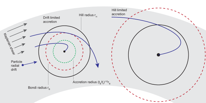
In the same way that we distinguish between shear- and dispersion-dominated regimes of planetesimal accretion (§III.2.3), how pebbles accrete depends upon whether the tidal field of the star needs to be taken into account. We first define two relevant radii. Ignoring both tidal (3-body) and gas drag effects a pebble approaching a protoplanet at velocity with impact parameter will suffer a strong deflection of the order of if , where
| (208) |
(This is justified to within factors of order unity in §IV.1.1.) Following (rather confusing) convention we refer to this critical radius for large-angle scattering as the Bondi radius. A second characteristic scale is provided by the Hill radius (equation 184),
| (209) |
which defines the boundary beyond which tidal effects are important. At the Hill radius Keplerian shear introduces a velocity relative to the protoplanet . Comparing this to the aerodynamic pebble approach speed (equation 207) we find,
| (210) |
Under the assumption that strong 2-body deflection is a pre-requisite for aerodynamically assisted accretion we can then distinguish the two regimes of pebble accretion illustrated in Figure 27:
-
•
If pebbles that can potentially be accreted approach the protoplanet with a velocity set by radial drift. Accretion can be modeled without considering tidal effects. This is the regime of drift limited accretion.
-
•
If Keplerian shear dominates the approach velocity for large impact parameters, and limits the capture cross-section to roughly the Hill radius. This is Hill limited accretion.
The transition between these regimes occurs when . The transition mass is,
| (211) |
with as given in eq. (207). There is a very strong dependence on the disk structure via the radial pressure support parameter . Restricting ourselves to power-law disk models (equation 130) with mid-plane we have that . A disk with and has , and we estimate the transition mass as,
| (212) |
We should remember that the fundamental dependence is on rather than on , and revert to the basic equations when considering locations such as planetary gap edges or pressure traps. With that caveat, however, we expect a modest increase in with radius in the disk, and a larger increase in the transition mass with distance from the star.
Requiring that particles suffer strong deflections due to the gravity of the planet is a necessary but not sufficient condition for them to be accreted in the presence of gas drag. We can determine the capture cross-section via a time scale argument. In the drift dominated case appropriate for small protoplanets there are three relevant time scales:
-
•
The friction time scale .
-
•
The time scale for a pebble to cross the Bondi radius .
-
•
The time scale for the planet, with gravity , to modify the velocity of a pebble with impact parameter , .
To be accreted we require that the planet’s gravity be strong enough to “pull” a pebble out of the aerodynamic flow, i.e. that (this assertion is supported by numerical integrations; Ormel & Klahr, 2010; Lambrechts & Johansen, 2012). Taking to define the capture cross-section we obtain,
| (213) |
The best situation for pebble accretion corresponds to , in which case a large fraction of particles entering the Bondi radius end up getting accreted. With the same power-law disk model we used before this condition implies,
| (214) |
Once again there is a strong dependence on the geometric thickness of the gas disk. For nominal parameters appropriate to a protoplanet with a mass similar to the transition mass (equation 212), and , the optimal dimensionless stopping time is .
Particles participating in pebble accretion are likely to have settled vertically, and depending upon the thickness of the settled layer (relative to ) the geometry of accretion may be either two- or three-dimensional. If the pebbles have surface density and mid-plane density simple geometry gives the appropriate accretion rate in the two regimes,
| (215) | |||||
| (216) |
What sort of growth is this? Substituting for in the expression above we find, in the three dimensional limit,
| (217) |
Both and are properties of the particle disk rather than of the planet, so we have simply that and a prediction of exponential growth.
Identical considerations govern the expected accretion rate in the Hill limited regime (Lambrechts & Johansen, 2012). In this case the crossing time of the Hill radius is , and the requirement that implies immediately that the best particle size has . Most commonly the two dimensional accretion geometry is relevant, so we have,
| (218) |
We expect a transition in growth rates as protoplanets accreting pebbles via this aerodynamic mechanism pass from the drift to Hill limited regimes.
The sketch of the physics of pebble accretion given above is greatly simplified, and the reader is directed to the original papers of Ormel & Klahr (2010) and Lambrechts & Johansen (2012) both for more details and for justification of some of the assertions that we have made. Hydrodynamic calculations confirm that although the smallest particles get swept past embedded protoplanets by the aerodynamic flow, estimates based on three-body integrations of particle trajectories with drag are valid for most of the relevant particle sizes (Ormel, 2013; Morbidelli & Nesvorny, 2012). Within a pebble accretion scenario the growth rates of protoplanets depend critically upon the local abundance of particles of the right size to participate in the process. This is hard to determine, as the particle sizes of interest are precisely those that are subject to rapid radial drift with presumptively short residence times in the disk. Nonetheless, many estimates suggest that pebble accretion could be the dominant growth mechanism for at least some classes of planets. Examples of papers that discuss how planetary growth proceeds under pebble accretion include Lambrechts & Johansen (2014), Bitsch, Lambrechts & Johansen (2015), Levison, Kretke & Duncan (2015a) and Levison et al. (2015b).
III.2.8 Coagulation equation
For both dust and planetary growth the basic mathematical question is how a size distribution evolves under the action of discrete collision events (possibly supplemented by a component of smooth accretion). The quantitative framework for addressing such questions is based on the coagulation equation Smoluchowski (1916). This allows us to drop our rather poorly defined descriptions of “large” and “small” bodies though at the expense of an enormous increase in complexity.
To write the coagulation equation in its simplest form191919It is also possible to write the coagulation equation as an integro-differential equation for a continuous mass function Safronov (1969), or as a discrete equation where bodies are binned into arbitrary mass intervals (typically logarithmic). Kenyon & Luu (1998) provide a clear description of how the coagulation equation may be formulated and solved in the more general case., assume that the masses of bodies are integral multiples of some small mass . At time there are bodies of mass . The coagulation equation in discrete form is,
| (219) |
where is the rate of mergers between bodies of mass and . The first term on the right-hand side of the equation describes the increase in the number of bodies of mass due to collisions of all possible pairs of bodies whose masses and sum to . The second term describes the decrease due to bodies of mass being incorporated into even larger bodies. The possibility of fragmentation is here neglected. In this formulation of the problem of planetary growth, all of the physics — such as gravitational focusing — enters via the rate coefficients .
Equation (219), or variants of it, has been used extensively to study planet formation Safronov (1969); Kenyon & Luu (1998); Wetherill & Stewart (1993); Inaba et al. (2001), either on its own or in combination with direct N-body simulations Bromley & Kenyon (2006). Generally the coagulation equation needs to be supplemented with additional equations that describe the evolution of the velocity dispersion as a function of mass, as described for example in Kenyon & Luu (1998). Because of the fact that all , such that contribute to the evolution of , even the coagulation equation on its own is not a simple equation to deal with, and few analytic solutions are known. One (over)-simple case for which an analytic solution exists is for the case when,
| (220) |
with a constant. Then, if the initial state of the system comprises bodies all of mass , the solution to equation (219) is,
| (221) |
This solution is shown as Figure 28. The mass spectrum remains smooth and well-behaved as growth proceeds, and with increasing time the characteristic mass increases linearly while maintaining a fixed shape.

More generally, solutions to the coagulation equation fall into two classes e.g. Lee (2000):
-
•
Solutions that exhibit orderly growth, in which the mass distribution evolves smoothly with time toward higher mean masses. The analytic solution given above for the case is an example of this type of evolution. Another analytic example is .
-
•
Solutions that show runaway growth. In this case the mass distribution develops a power-law tail toward high masses — physically this corresponds to one or a handful of bodies growing rapidly at the expense of all the others. The long-term validity of the coagulation equation once runaway growth occurs is evidently limited. An analytic example occurs for a rate coefficient .
Looking back to equation (190), we note that the rate coefficient is expected to scale as in the regime where gravitational focusing is unimportant, and once gravitational focusing is dominant. By comparison with the aforementioned analytic solutions, we expect that the initial growth of planetesimals will occur in the orderly regime, while runaway growth may occur once the largest bodies are massive enough for gravitational focusing to become significant.
III.2.9 Overview of terrestrial planet formation
We conclude the discussion of terrestrial planet formation by summarizing briefly the main stages of the process:
-
1.
Dust particles agglomerate to form, eventually, planetesimals. Initially this occurs via pairwise collisions, though how (or whether) this process can continues to work for cm to meter scale particles remains somewhat murky. Gravitational instability, probably initiated by the streaming instability, may allow a bypass of these tricky sizes.
-
2.
Growth beyond planetesimals occurs via direct collisions, with an increasing role for gravitational focusing as masses become larger. Pebble accretion contributes to growth, by an amount that depends upon the abundance and size of surviving small solids. Dynamical friction keeps the velocity dispersion of the most massive bodies low. A phase of runaway growth may occur in which a few bodies grow rapidly at the expense of the rest.
-
3.
Runaway growth ceases once the largest bodies become massive enough to stir up the planetesimals in their vicinity. A phase of oligarchic growth ensues, in which the largest objects grow more slowly than they did during runaway growth, but still more rapidly than small bodies Kokubo & Ida (1998); Thommes, Duncan & Levison (2003). Growth continues in this mode until the isolation mass is approached, at which point growth slows further.
-
4.
Further evolution occurs as a result of collisions between the initially relatively isolated planetary embryos left over after oligarchic growth. The embryos are perturbed onto crossing orbits due to the influence of the giant planets and mutual secular resonances Chambers & Wetherill (1998). The final assembly of the terrestrial planets takes around 100 Myr, with the predicted configuration varying depending upon the assumed surface density of planetesimals and existence (or not) of giant planets Kokubo, Kominami & Ida (2006); Levison & Agnor (2003); Raymond, Quinn & Lunine (2005). In the Solar System, one of the final impacts on the Earth is widely considered to have given rise to the ejection of enough mass into orbit to subsequently form the Moon Canup (2004).
The dominant uncertainties in theoretical models for terrestrial planet formation are arguably found during stage 1 — the formation of planetesimals. It is also true that most simulations of the late stages of terrestrial planet formation lead to planetary properties (such as the eccentricity, and the mass of Mars compared to the other terrestrial planets) that differ somewhat from those observed in the Solar System. Thus, although there is general confidence that the basic physics of terrestrial planet formation is understood, it is clear that current models do not include all of the ingredients needed to accurately match Solar System constraints (Raymond et al., 2009).
III.3 Gas giant formation
The formation of at least the vast majority of known gas giant planets is thought to occur as a consequence of core accretion Mizuno (1980); Bodenheimer & Pollack (1986). The core accretion model, which had a lengthy gestation period leading up to the landmark paper of Pollack et al. (1996), postulates that the envelopes of gas giants are accreted subsequent to the formation of a large core, which is itself assembled in a manner analogous to terrestrial planet formation.
Core accretion is the most widely accepted theory for massive planet formation. There is, however, an alternative model, based on the idea that a massive protoplanetary disk might collapse directly to form massive planets Kuiper (1951); Cameron (1978); Boss (1997). In this Section, we review the physics of these theories in turn. We also discuss the observational constraints on the different theories, which include inferences as to the core masses of the gas giants in the Solar System and the properties of extrasolar planetary systems.
III.3.1 Core accretion model
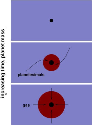
The main stages in the formation of a gas giant via core accretion are illustrated in Figure 29. A core of rock and / or ice forms via the same mechanisms that we have previously outlined for terrestrial planet formation. Initially, there is either no atmosphere at all (because the potential is too shallow to hold on to a bound atmosphere), or any gas is dynamically insignificant. However, as the core grows, eventually it becomes massive enough to hold on to a significant envelope. At first, the envelope is able to maintain hydrostatic equilibrium. The core continues to grow via accretion of planetesimals (or pebbles), and the gravitational potential energy liberated as these solids rain down on the core provides the main source of luminosity. (In the limiting case where there is no planetesimal luminosity, analyzed in detail by Piso & Youdin (2014), energy comes instead from Kelvin-Helmholtz contraction of the envelope.) This growth continues until the core reaches a critical mass. Once the critical mass is reached the envelope can no longer be maintained in hydrostatic equilibrium. The envelope contracts on its own Kelvin-Helmholtz time scale, and a phase of rapid gas accretion occurs. This process continues until (a) the planet becomes massive enough to open up a gap in the protoplanetary disk, thereby slowing down the rate of gas supply, or (b) the gas disk itself is dispersed.
The novel aspect of the core accretion model is the existence of a critical core mass. Mizuno (1980) used numerical models to demonstrate the existence of a maximum core mass, and showed that it depends only weakly on the local properties of the gas within the protoplanetary disk. A clear exposition of this type of calculation is given in, for example, Papaloizou & Terquem (1999). The simplest toy model that exhibits the key property of a critical core mass is that due to Stevenson (1982), who considered the (unrealistic) case where energy transport is due solely to radiative diffusion. We reproduce his argument here. Rafikov (2006) is a good place to start for understanding more realistic models in which convection also plays a role.
Consider a core of mass and radius , surrounded by a gaseous envelope of mass . The total mass of the planet,
| (222) |
The envelope extends from to some outer radius , which marks the boundary between the gas bound to the planet and the gas in the protoplanetary disk. may be determined by thermal effects (in which case , with the disk sound speed) or by tidal considerations (giving an outer radius of ), whichever is the smaller. If the envelope is of low mass, then the largest contribution to the luminosity is from accretion of planetesimals onto the core. This yields a luminosity,
| (223) |
which is constant through the envelope.
If we assume that radiative diffusion dominates the energy transport, then the structure of the envelope is determined by the equations of hydrostatic equilibrium and radiative diffusion,
| (224) | |||||
| (225) |
where is the Stefan-Boltzmann constant and the Rosseland mean opacity (assumed constant). Eliminating the density between these equations we find that,
| (226) |
We now integrate this equation inward from the outer boundary, making the approximation that and taking and to be constants,
| (227) |
Once we are well inside the planet we expect that and that , so the integral yields, approximately,
| (228) |
Substituting in this equation with an ideal gas equation of state,
| (229) |
we eliminate in favor of the expression involving and integrate once more with respect to radius to obtain,
| (230) | |||||
| (231) |
Having derived the density profile the mass of the envelope follows immediately,
| (232) | |||||
The right-hand-side of this equation has a strong dependence on the total planet mass and a weaker dependence on the core mass via the expression for the luminosity,
| (233) |
In principle there are further dependencies to consider since is a function of and is a function of , but these enter only logarithmically and can be safely ignored. Noting that,
| (234) |
we find that,
| (235) |
where we have shown explicitly the dependence on the envelope opacity and planetesimal accretion rate but have swept all the remaining constants (and near-constants) into a single constant .
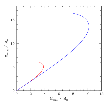
Solutions to equation (235) are plotted as Figure 30. One sees that for fixed , there exists a maximum or critical core mass beyond which no solution is possible. The physical interpretation of this result is that as the mass of the envelope increases relative to that of the core, ever higher pressures at the core-envelope boundary are needed to maintain the envelope in hydrostatic balance. At the critical mass, adding more gas to the envelope to raise the base pressure fails to help, because the added gas contributes more to the self-gravity tending to compress the envelope than to the pressure holding it up. Once the critical mass is exceeded hydrostatic equilibrium cannot be achieved in the envelope. Rather the envelope will contract, and further gas will fall in as fast as gravitational potential energy can be radiated.
This toy model should not be taken too seriously. However, it does illustrate the most important result from more detailed calculations — namely that the critical mass increases with larger and with enhanced opacity. Ikoma, Nakazawa & Emori (2000) derive an approximate fit to numerical results,
| (236) |
where the power-law indices are uncertain by around . The weak dependence of the critical core mass on the planetesimal accretion rate means that, within a particular core accretion model, we can always speed up the approach to runaway gas accretion simply by increasing the assumed surface density of planetesimals in the vicinity of the growing core. Contrary to what is sometimes implied, there is no intrinsic difficulty in building planets quickly via core accretion. However, faster growth occurs at the expense of a larger final core mass.
Although they appear very detailed, extant calculations of planet growth via core accretion should probably be regarded as illustrative rather than definitive. Three sources of particular uncertainty are present,
-
•
What is the magnitude of the opacity? Although enters equation (236) as rather a weak power, its magnitude is highly uncertain. Hubickyj, Bodenheimer & Lissauer (2005), and more Movshovitz et al. (2010), have computed core accretion models in which the opacity is either arbitrarily reduced or computed from a settling and coagulation model. These models suggest, first, that the appropriate value of the opacity in the envelope is greatly reduced (by a factor of the order of ) from the interstellar value (Podolak, 2003). Second, they indicate that the reduced opacity results in substantially faster growth of massive planets. Formation time scales as short as a Myr, or (for longer formation times) core masses as small as 5 , are achievable.
-
•
The neglect of core migration. Theoretical work, which we will discuss more fully in a subsequent Section, suggests that planets or planetary cores with masses exceeding are highly vulnerable to radial migration as a consequence of gravitational torques exerted by the gas disk. This effect is not included in the calculations of Pollack et al. (1996) or Hubickyj, Bodenheimer & Lissauer (2005). Papaloizou & Terquem (1999) and Alibert et al. (2005) have studied the effect of steady inward migration on core formation, and have showed that it makes a large change to the time scale and outcome of the process. Radial migration could also be driven by dynamical interactions between growing cores and planetesimals (Levison, Thommes & Duncan, 2010).
-
•
The relative role of planetesimal versus small particle accretion. In the classic model of Pollack et al. (1996), and its later refinements, the core grows exclusively by accreting planetesimals. However, as we noted in §III.2.7, the accretion of smaller aerodynamically coupled solids could be equally or more important for core growth (Ormel & Klahr, 2010; Lambrechts & Johansen, 2012; Chambers, 2014). The size of primordial planetesimals is an important factor in determining the relative contribution of planetesimals versus pebbles. Small planetesimals—with radii of the order of a km—retain enough aerodynamic damping to stay dynamically cold, and have large gravitational focusing factors. Larger planetesimals, such as those produced to arise from simulations of the streaming instability (Simon et al., 2016; Schäfer, Yang & Johansen, 2017), are less favorable building blocks for rapid core formation, and if most of the mass in the planetesimal population is in bodies pebble accretion may well be needed.
To summarize, the broad outlines of how core accretion works are well established, but even the most sophisticated models are probably lacking some essential physical elements.
III.3.2 Gravitational instability model
A sufficiently massive and / or cold gas disk is gravitationally unstable. Gravitational instability can lead to two possible outcomes: stable angular momentum transport or fragmentation. Kratter & Lodato (2016) provide a comprehensive review of both possibilities, here we focus on the idea that fragmentation could provide a mechanism for giant planet formation Kuiper (1951); Cameron (1978).
We have already derived the necessary conditions for gravitational instability to occur. We need the Toomre parameter to be low enough, specifically,
| (237) |
where is the sound speed in a gas disk of local surface density and the disk mass is assumed to be small enough that the distinction between the orbital and epicyclic frequencies is of little import. If we consider a disk with at 10 AU around a Solar mass star, then the relation yields a sound speed . To attain , we then require a surface density,
| (238) |
This is much larger than estimates based, for example, on the minimum mass Solar Nebula, from which we conclude that gravitational instability is most likely to occur at an early epoch when the disk mass is still high. Recalling that the characteristic wavelength for gravitational instability is , we find that the mass of objects formed if such a disk fragmented would be,
| (239) |
where is the mass of Jupiter. At an order of magnitude level it appears that gravitational instability followed by fragmentation could form objects with masses in the giant planet range. For those objects to remain planets, however, requires that they accrete relatively modest amounts of gas from their young, gas-rich environment. Keeping fragments formed from gravitational collapse from growing into brown dwarfs or low mass stars is thus a significant challenge (Kratter, Murray-Clay & Youdin, 2010).
It is also straightforward to derive where in the disk gravitational instability is most likely to occur. Noting that in a steady-state accretion disk , we use the prescription Shakura & Sunyaev (1973) and obtain,
| (240) |
The sound speed in a protoplanetary disk decreases outward, so a steady-state disk becomes less stable at large radii. Indeed, unless the temperature becomes so low that external irradiation (not that from the central star) dominates the heating, a steady-state disk will become gravitational unstable provided only that it is large enough.
To derive sufficient conditions for fragmentation, we need to go beyond these elementary considerations and ask what happens to a massive disk as instability is approached. The critical point is that as is reduced, non-axisymmetric instabilities set in which do not necessarily lead to fragmentation. Rather, the instabilities generate spiral arms which transport angular momentum and lead to dissipation and heating. The dissipation results in heating of the disk, which raises the sound speed and can lead to a stable self-gravitating state in which heating and cooling balance (Paczynski, 1978). On a longer time scale, angular momentum transport also leads to lower surface density and, again, enhanced stability Lin & Pringle (1990).
Given these consideration, when will a disk fragment? Gammie (2001) used both analytic arguments and local numerical simulations to identify the cooling time as the control parameter determining whether a gravitationally unstable disk will fragment. For an annulus of the disk we can define the equivalent of the Kelvin-Helmholtz time scale for a star,
| (241) |
where is the thermal energy content of the disk per unit surface area. Then for an ideal gas equation of state with Gammie (2001) found that the boundary for fragmentation is:
-
•
— the disk fragments.
-
•
— disk reaches a steady state in which heating due to dissipation of gravitational turbulence balances cooling.
This condition is intuitively reasonable. Spiral arms resulting from disk self-gravity compress patches of gas within the disk on a time scale that is to order of magnitude . If cooling occurs on a time scale that is shorter that , the heating due to adiabatic compression can be radiated away, and in the absence of extra pressure collapse is likely. The above condition was derived locally, but initial global simulations suggested that it provides a good approximation to the stability of protoplanetary disks more generally Rice et al. (2003b). One can also express the fragmentation boundary in terms of a maximum stress that a self-gravitating disk can sustain without fragmenting Gammie (2001). Writing this in terms of an effective parameter, Rice, Lodato & Armitage (2005).
In a real disk, the cooling time is determined by the opacity and by the mechanism of vertical energy transport: either radiative diffusion or convection. Using a disk model, one can then estimate analytically the conditions under which a disk will become unstable to fragmentation (Rafikov, 2005; Levin, 2007; Rafikov, 2009; Clarke, 2009). For standard opacities, the result is that fragmentation is expected only at quite large radii of the order of 50 or 100 AU. On these scales a large reservoir of mass is typically available locally and the likely outcome would be very massive planets or brown dwarfs (Stamatellos & Whitworth, 2009). At smaller radii the disk may still be gravitationally unstable, but the instability will saturate prior to fragmentation and, instead, contribute to angular momentum transport.
The idea that the criterion for fragmentation can be written in terms of a threshold value of , as discussed above, is useful but somewhat too simple. On the 50-100 AU scales where fragmentation is most likely to occur stellar irradiation cannot be ignored, and modifies the criteria for fragmentation (Rice et al., 2011). Moreover, the numerical simulations used to study fragmentation exhibit quite subtle convergence properties (as originally shown by Meru & Bate, 2011), and the detailed results can be sensitive both to stochastic effects (Pardekooper, 2012) and to the treatment of cooling (Rice et al., 2014). Further high resolution simulations that include both radiative transport (Boley et al., 2010) and MHD (Forgan, Price & Bonnell, 2017) are probably needed.
III.3.3 Comparison with observations
The architecture of the Solar System’s giant planets provides qualified support for the core accretion model. The time scale for core accretion increases with orbital radius, which is qualitatively consistent with the general trend of planetary properties in the outer Solar System — Jupiter is closest to Solar composition (reflecting a fully formed gas giant), while Saturn and the ice giants are relatively gas poor. Perhaps these outermost planets formed as the gas disk was in the process of being dispersed.
The most direct test of core accretion in the Solar System involves measurement of the core masses of Jupiter and Saturn. Information as to the interior structure of the gas giants can be derived from exterior measurements of the gravitational multipole moments (for Jupiter, from the Galileo orbiter). When combined with interior structure models, which rely on knowledge of the equation of state at high pressures and densities, the measured multipole moments yield constraints on the core mass. Currently, the uncertainties on reasonable interior structure models appear to be large enough as to frustrate definitive conclusions. Militzer et al. (2008) have calculated Jovian models that include a substantial () core, while Nettelmann et al. (2008) have computed similarly state-of-the-art models that support earlier suggestions (Guillot, 2005) that any core must be small. The differences appear to result primarily from different assumptions made by the two groups as to the number of distinct layers within the interior of Jupiter. NASA’s JUNO mission will return additional data that will yield new constraints on the interior structure of Jupiter, and it is to be hoped that this data will result in improved measurements of the planet’s core mass.
Observations of extrasolar planets also yield constraints. Core accretion predicts that a greater surface density of planetesimals would lead to faster core growth and an increased chance of reaching runaway prior to disk dispersal. This is consistent with the observed correlation of massive planet frequency with host metallicity Fischer & Valenti (2005); Ida & Lin (2004). There are also known extrasolar planets whose small radii imply a large mass of heavy elements (HD 149026 being one example; Sato et al., 2005), properties consistent with the outcome of core accretion.
This does not, of course, mean that disk instability does not occur. As we have emphasized fragmentation is expected to occur only at large disk radii, whereas almost all known exoplanets have been discovered via search techniques that are most sensitive to planets with small to intermediate separations. If disk instability does occur then we would expect a second population of massive planets in wide orbits (Boley et al., 2009) with a different host metallicity distribution (Rice et al., 2003c). Among known systems HR 8799 (Marois et al., 2008) is the closest to matching the expectations for a system formed via disk instability, but the evidence (for either fragmentation or core accretion) is inconclusive and to date there are no planets that clearly demand a disk instability origin.
IV Evolution of Planetary Systems
The story is not over once planets have managed to form. Theoretical models, which are now strongly supported by observations of the Solar System and of extrasolar planetary systems, suggest at least five mechanisms that can lead to substantial post-formation orbital evolution:
-
•
Interaction between planets and the gaseous protoplanetary disk. This leads to orbital migration Goldreich & Tremaine (1980) as a consequence of angular momentum exchange between the planet and the gas disk, and can be important for both terrestrial-mass planets and gas giants while the gas disk is still present. Gas disk migration was the first process suggested as an explanation for the existence of hot Jupiters Lin, Bodenheimer & Richardson (1996).
-
•
Interaction between planets and a remnant planetesimal disk. Planets, especially giant planets, can also exchange angular momentum by interacting with and ejecting planetesimals left over from the planet formation process. This mechanism appears likely to have caused orbital migration of at least the ice giants, and possibly also Saturn, during the early history of the Solar System Levison et al. (2007).
-
•
Interaction within an initially unstable system of two or more massive planets. There is no guarantee that the architecture of a newly formed planetary system will be stable over the long run. Instabilities can lead to planet-planet scattering, which usually results in the ejection of the lower mass planets, leaving the survivors on eccentric orbits. This could be the origin of the typically eccentric orbits seen in extrasolar planetary systems Lin & Ida (1997); Rasio & Ford (1996); Weidenschilling & Marzari (1996). A fraction of scattered planets are typically injected on to highly eccentric and inclined orbits that may subsequently circularize to form hot Jupiters.
-
•
Interaction between orbiting planets and stellar binary companions. A planet whose orbital plane is substantially misaligned with that of a binary companion has its eccentricity excited by the Kozai-Lidov mechanism (Kozai, 1962; Lidov, 1962). The eccentricity can become large enough that, at closest approach, energy is dissipated in tidal interactions with the star, forming hot Jupiters (Wu & Murray, 2003).
-
•
Tidal interactions between planets and their host stars, which are of particular importance for hot Jupiters given that their orbital radii are, in some cases, just a handful of stellar radii.
This Section gives an elementary introduction to a selection of these mechanisms (for a higher-level review, see Davies et al., 2014). The focus here is exclusively on dynamical evolution of newly formed planetary systems.
IV.1 Gas disk migration
The calculation of the torque experienced by a planet embedded within a viscous disk is highly technical, and although the basic principles are secure the details are anything but. Here, we first give a semi-quantitative treatment based on the impulse approximation (Lin & Papaloizou, 1979). We then sketch some of the key ideas that underlie more detailed computations, which are based on summing the torque over a set of discrete resonances between the planet and the gaseous disk (Goldreich & Tremaine, 1979). Several excellent reviews are recommended for the reader seeking more details (Lubow & Ida, 2010; Kley & Nelson, 2012; Baruteau et al., 2014).
IV.1.1 Torque in the impulse approximation
Working in a frame of reference moving with the planet, we consider the gravitational interaction between the planet and gas flowing past with relative velocity and impact parameter . The change to the perpendicular velocity that occurs during the encounter can be computed by summing the force along the unperturbed trajectory. It is,
| (242) |
where is the planet mass. This velocity is directed radially, and hence does not correspond to any angular momentum change. The interaction in the two-body problem is however conservative, so the increase in the perpendicular velocity implies a reduction (in this frame) of the parallel component. Equating the kinetic energy of the gas particle well before and well after the interaction has taken place we have that,
| (243) |
which implies (for small deflection angles),
| (244) |
If the planet has a semi-major axis the implied angular momentum change per unit mass of the gas is,
| (245) |
It is worth pausing at this juncture to fix the sign of the angular momentum change experienced by the gas and by the planet firmly in our minds. Gas exterior to the planet’s orbit orbits the star more slowly than the planet, and is therefore “overtaken” by the planet. The decrease in the parallel component of the relative velocity of the gas therefore corresponds to an increase in the angular momentum of the gas exterior to the planet. Since the gravitational torque must be equal and opposite for the planet the sign is such that:
-
•
Interaction between the planet and gas exterior to the orbit increases the angular momentum of the gas, and decreases the angular momentum of the planet. The planet will tend to migrate inward, and the gas will be repelled from the planet.
-
•
Interaction with gas interior to the orbit decreases the angular momentum of the gas and increases that of the planet. The interior gas is also repelled, but the planet tends to migrate outward.
In the common circumstance where there is gas both interior and exterior to the orbit of the planet the net torque (and sense of migration) will evidently depend upon which of the above effects dominates.
The total torque on the planet due to its gravitational interaction with the disk can be estimated by integrating the single particle torque over all the gas in the disk. For an annulus close to but exterior to the planet, the mass in the disk between and is,
| (246) |
where (assumed to be a constant) is some characteristic value of the gas surface density. If the gas in the annulus has angular velocity and the planet has angular velocity all of the gas within the annulus will encounter the planet in a time interval,
| (247) |
Approximating as,
| (248) |
which is valid provided that , we obtain the total torque on the planet due to its interaction with gas outside the orbit by multiplying by , dividing by , and integrating over impact parameters. Formally we would have that,
| (249) |
but this integral is clearly divergent – there is what must be an unphysically infinite contribution from gas passing very close to the planet. Sidestepping this problem for now, we replace the lower limit with a minimum impact parameter and integrate. The result is,
| (250) |
It is possible to tidy up this calculation somewhat, for example by taking proper account of the rotation of the planet frame around the star, and if this is done the result is that the expression derived above must be multiplied by a correction factor (Papaloizou & Terquem, 2006).
Aside from the sign of the torque the most important result that we can glean from this calculation is that the torque on the planet due to its interaction with the gas scales as the square of the planet mass. This scaling can be compared to the orbital angular momentum of the planet, which is of course linear in the planet mass. We conclude that if all other factors are equal – in particular if neither in the vicinity of the planet nor vary with – the time scale for the planet to change its orbital angular momentum significantly will scale inversely with the planet mass. The migration velocity in this limit will then be proportional to – more massive planets will migrate faster.
Finally we can estimate the magnitude of the torque for parameters appropriate to different stages of giant planet formation. First, let us consider a rather low mass core () growing at 5 AU in a gas disk of surface density around a Solar mass star. Our treatment of the interaction has assumed that the disk can be treated as a two-dimensional sheet, so it is arguably natural to take as a minimum impact parameter . Using these numbers we find that the exterior torque would drive inward migration on a time scale,
| (251) |
Of course this will be partly offset by the interior torque – which has the opposite sign – but absent some physical reason why these two torques should cancel to high precision we would predict changes to the semi-major axis on a time scale of the order of a Myr. This is already rapid enough to be a potentially important effect during giant planet formation via core accretion. Second, we can evaluate the torque for a fully-formed gas giant. A Jupiter mass planet has a Hill sphere , so it seems reasonable to argue that the value of that we adopted for an Earth mass core is too small in this case. Picking a modestly larger value results in a time scale,
| (252) |
that is an order of magnitude shorter than typical protoplanetary disk lifetimes. If these estimates can be trusted to even an order of magnitude the conclusion is inescapable – gas disk migration ought to be an important process for the early evolution of the orbits of giant planets.
IV.1.2 Torque at resonances
A more involved – but ultimately more powerful – approach to calculate the torque is to decompose it into a sum over partial torques exerted at resonant locations with the disk (Goldreich & Tremaine, 1979; Tanaka, Takeuchi & Ward, 2002). For simplicity, we start by considering a planet orbiting a star on a circular orbit with angular frequency . A standard exercise in dynamics (e.g. Binney & Tremaine 1987) yields the conditions for resonances. A corotation resonance exists for radii in the disk where the angular frequency ,
| (253) |
Lindblad resonances exist when,
| (254) |
where is an integer and , the epicyclic frequency, is defined as,
| (255) |
with the stellar gravitational potential. For a Keplerian potential . If we approximate the angular velocity of gas in the disk by the Keplerian angular velocity, the Lindlad resonances are located at,
| (256) |
where is the planet orbital radius. The locations of some of the low order (small ) resonances are shown in Figure 31. For an orbiting test particle, the resonances are locations where the planet can be a strong perturbation to the motion. For a gas disk, angular momentum exchange between the planet and the gas disk occurs at resonant locations. As we noted for the impulse approximation, the sense of the interaction is that the planet gains angular momentum from interacting with the gas disk at the interior Lindblad resonances (). This tends to drive the planet outward. The gas loses angular momentum, and moves inward. Conversely, the planet loses angular momentum from interacting with the gas disk at exterior Lindblad resonances (). This tends to drive the planet toward the star. The gas gains angular momentum, and moves outward. Notice that the gravitational interaction of a planet with a gas disk tends — somewhat counter-intuitively — to repel gas from the vicinity of the planet’s orbit.
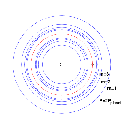
The flux of angular momentum exchanged at each Lindblad resonance can be written as,
| (257) |
where is the gas density and the planet mass. That the torque should scale with the square of the planet mass is intuitively reasonable — the perturbation to the disk surface density scales as the planet mass in the linear regime so the torque scales as . The factor is the torque cutoff function Artymowicz (1993), which encodes the fact that resonances very close to the planet contribute little to the net torque. The torque cutoff function peaks at,
| (258) |
i.e. at a radial location , where is the disk scale height (this result immediately implies that a three-dimensional treatment is necessary for the dominant resonances if the planet is completely embedded within a gas disk, as is the case for low mass planets). The strength of the torque exerted at each resonance is essentially independent of properties of the disk such as the disk viscosity, though of course the viscosity still matters inasmuch as it controls the value of the unperturbed disk surface density .
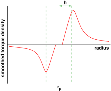
Figure 32 illustrates the differential torque exerted on the disk by the planet, after smoothing over the Lindblad resonances Ward (1997). The flux of angular momentum is initially deposited in the disk as waves, which propagate radially before dissipating. The details of this dissipation matter little for the net rate of angular momentum exchange.
Angular momentum transfer at corotation requires additional consideration, and as we will see later thinking of these torques in terms of resonances is not as profitable as for the Lindblad torques. Formally though, in a two-dimensional disk the rate of angular momentum deposition at corotation is proportional to Goldreich & Tremaine (1979); Tanaka, Takeuchi & Ward (2002),
| (259) |
where is the Oort parameter,
| (260) |
This implies that in a two-dimensional disk, the resonant corotation torque vanishes identically in the moderately interesting case of a disk with a surface density profile . This result does not apply to three-dimensional disks Tanaka, Takeuchi & Ward (2002).
IV.1.3 Type I migration
For low mass planets (generically , though the exact mass depends upon the disk properties) the angular momentum flux injected into the disk as a consequence of the planet-disk interaction is negligible when compared to the viscous transport of angular momentum. As a result, the gas surface density profile remains approximately unperturbed, gas is present at the location of each of the resonances, and the net torque on the planet is obtained by summing up the torque exerted at each resonance. Schematically,
| (261) |
where the planet gains angular momentum from the inner Lindblad resonances (ILR) and loses angular momentum to the outer Lindblad resonances (OLR). There is also a potentially important co-orbital torque . Changes to the planet’s orbit as a result of this net torque are called Type I migration Ward (1997).
As noted above (equation 257) the torque exerted at each resonance scales as the planet mass squared. If the azimuthally averaged surface density profile of the gas disk remains unperturbed, it follows that the total torque will also scale as and the migration time scale,
| (262) |
Type I migration is therefore most rapid for the largest body for which the assumption that the gas disk remains unaffected by the planet remains valid.
Actually evaluating the sum sketched out in equation (261) is not easy, and there is no simple physical argument that I am aware of that gives even the sign of the net torque on the planet. However invariably it is found that the Lindblad resonances exterior to the planet are more powerful than those interior, so that the net torque due to Lindblad resonances leads to inward migration. Note that one might think (for example by looking at the surface density dependence of the torque in equation 257) that the sense of migration ought to depend upon the surface density gradient — i.e. that a steep surface density profile should strengthen the inner resonances relative to the outer ones and hence drive outward migration. This is not true. Pressure gradients (which depend upon the radial dependence of the surface density and temperature) alter the angular velocity in the disk from its Keplerian value (equation 131), and thereby shift the radial location of resonances from their nominal positions. A steep surface density profile implies a large pressure gradient, so that all the resonances move slightly inward. This weakens the inner Lindblad resonance relative to the outer ones, in such a way that the final dependence on the surface density profile is surprisingly weak Ward (1997).
Tanaka, Takeuchi & Ward (2002) compute the net torque on a planet in a three-dimensional but isothermal gas disk. For a disk in which,
| (263) |
they obtain a net torque due to Lindblad resonances only of,
| (264) |
This torque would result in migration on a time scale,
| (265) | |||||
where , and are respectively the gas surface density, gas sound speed, and angular velocity at the location of a planet orbiting at distance from a star of mass . As expected based on the simple considerations discussed previously, the migration rate () scales linearly with both the planet mass and the local disk mass. The time scale becomes shorter for cooler, thinner disks — provided that the interaction remains in the Type I regime — since for such disks more resonances close to the planet contribute to the net torque.
The most important thing to notice from this formula is that the predicted migration time scale is very short. If we consider a core growing at 5 AU in a disk with typical parameters (, , ) we find,
| (266) |
One concludes that there is a strong argument that Type I migration ought to play an important role in the formation of giant planet cores.
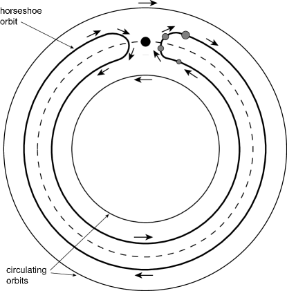
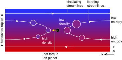
The Lindblad torque is only part of the total torque exerted on the planet. What about the co-orbital torque? The physics behind the origin of torques from gas that is almost co-orbiting with the planet is illustrated in Figure 33. The key point is that gas that is almost, but not quite, co-orbital executes horseshoe orbits when viewed in a frame co-rotating with the motion of the planet. As the gas executes the U-shaped turns at the ends of the horseshoe, changes in the gas density occur that are not symmetric between the disk trailing and leading the planet. The density variations source a torque that, because it arises from quite close to the planet, can be as large or larger than the torque from the Lindblad resonances.
Ward (1991) discussed how to calculate corotation torques from the physical perspective of gas on horseshoe orbits, but this way of thinking about the torque did not become widely known until simulations by Paardekooper & Mellema (2006) uncovered a dependence of the Type I migration rate on the thermal properties of the disk. Subsequently, many authors have studied the co-orbital Type I torque in both isothermal (Casoli & Masset, 2009; Paardekooper & Papaloizou, 2009) and non-isothermal (radiative or adiabatic) disks (Kley & Crida, 2008; Masset & Casoli, 2009; Kley, Bitsch & Klahr, 2009; Paardekooper et al., 2010; Paardekooper, Baruteau & Kley, 2011). The review by Baruteau et al. (2014) summarizes the results of these and other calculations.
The total torque on planets embedded in gaseous disks, and the corresponding Type I migration rate, is given by the sum of the Lindblad and corotation torques. In addition to the planet mass, several properties of the disk enter into the result:
- •
-
•
The cooling time of parcels of gas in the horseshoe region (due to radiative diffusion in the optically thick limit or explicit heating / cooling processes otherwise). This matter because part of the corotation torque depends upon the presence of thermal gradients as gas moves around horseshoe orbits. The strength of those gradients depends upon how quickly the gas heats and cools relative to the time scale needed to execute a horseshoe orbit.
-
•
The efficiency of angular momentum transport in the co-orbital region. The region of the disk that admits horseshoe orbits is closed and relatively small. It cannot absorb or give an arbitrary amount of angular momentum to a planet, unless it is “connected” to the rest of the disk via viscous stresses. Large and persistent co-orbital torques are possible provided that the disk is viscous enough that the torque remains unsaturated; very low viscosity leads to saturation and vanishing torques.
With all these factors to consider the calculation of the Type I migration rate is necessarily rather involved. One should remember, however, that both the Lindblad and corotation torques are large and would individually drive rapid migration. They may happen to sum to zero at special locations within the disk, but absent such happy coincidences migration of planets of roughly an Earth mass and higher will be significant. Type I migration can rarely be ignored in any circumstance where substantial gas disks co-exist with planets.
Bitsch et al. (2013) provide an example of how the Type I migration rate as a function of planet mass can be calculated given a specific disk model. They find that for sufficiently low mass planets ( in their fiducial example) the Lindblad torque dominates, and migration is inward at all radii. For more massive planets there are radial zones of outward migration interspersed with radii where migration is inward. The boundaries where (as we move out) migration switches from outward to inward define convergence zones where planets might tend to accumulate.
IV.1.4 Type II migration
For sufficiently large planet masses, the angular momentum flux from the planet locally dominates the viscous flux. As a consequence, gas is repelled from high-m resonances. The surface density drops near , forming a gap — an annular region in which the surface density is smaller than its unperturbed value.
Two conditions are necessary for gap formation. First, the Hill sphere (or Roche radius) of the planet needs to be comparable to the thickness of the gas disk,
| (267) |
which requires a mass ratio ,
| (268) |
This condition is satisfied for typical protoplanetary disk parameters for — i.e. for planet masses somewhere between that of Saturn and Jupiter.
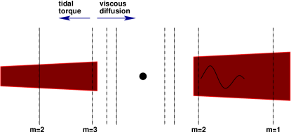
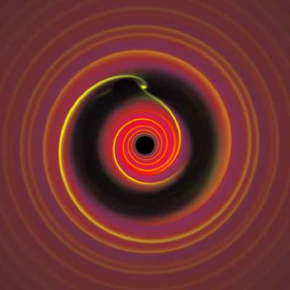
A second condition for gap opening arises due to the viscous considerations depicted in Figure 34. To open a gap, we require that the tidal torques must be able to remove gas from the gap region faster than viscosity can fill the gap back in Lin & Papaloizou (1980); Goldreich & Tremaine (1980); Papaloizou & Lin (1984). There are various ways to estimate the critical mass above which this condition is satisfied. Following Takeuchi, Miyama & Lin (1996), we note that the time scale for viscous diffusion to close a gap of width is just,
| (269) |
where is the disk viscosity. The time scale to open a gap as a result of the tidal torque at an -th order Lindblad resonance is,
| (270) |
Setting , and taking (since, as noted above, this value of is where the torque cutoff function peaks), we obtain,
| (271) |
For typical disk parameters (, ), the viscous condition for gap opening is satisfied for modestly larger than . Combined with the thermal condition outlined above, we conclude that Jupiter mass planets ought to be massive enough to open a gap within the disk, whereas Saturn mass planets are close to the critical mass required for gap opening. Figure 35 from Armitage & Rice (2005), shows results from a two-dimensional simulation of the planet-disk interaction in the Type II regime. Both the gap, and the presence of a prominent spiral wave excited within the gas disk, are obvious.
IV.1.5 The Type II migration rate
Once a planet becomes massive enough to open a gap, the orbital evolution becomes coupled to the viscous evolution of the gas within the disk. At small orbital radii the sense of gas motion will invariably be inward, and the planet will very probably follow suit (by similar arguments, the planet can migrate outward in regions where the gas disk is expanding, Veras & Armitage, 2004). The radial velocity of gas in the disk is,
| (272) |
which for a steady disk away from the boundaries can be written as,
| (273) |
If the planet enforces a rigid tidal barrier at the outer edge of the gap (i.e. no gas is accreted by the planet, and no gas crosses the gap), then evolution of the disk will force the orbit to shrink at a rate , provided that the local disk mass exceeds the planet mass, i.e. that . This implies a nominal Type II migration time scale, valid for disk dominated migration only,
| (274) |
For and , the migration time scale at 5 AU is of the order of 0.5 Myr.
In practice, the assumption that the local disk mass exceeds that of the planet often fails. For example, a plausible model of the protoplanetary disk with a mass of within 30 AU has a surface density profile,
| (275) |
The condition that gives an estimate of the radius within which disk domination ceases of,
| (276) |
Interior to this radius, the planet acts as a slowly moving barrier which impedes the inflow of disk gas. If the barrier was assumed (unrealistically, as we will see) to be impermeable then gas would pile up outside it. This pile-up would increase the torque but would not continue without limit because the interaction also deposits angular momentum into the disk, causing it to expand Pringle (1991). The end result would be slower migration compared to the nominal rate quoted above. Syer & Clarke (1995) and Ivanov, Papaloizou & Polnarev (1999) provide explicit formulae for calculating the extent of the suppression given the assumption of an impermeable tidal barrier.
These simple estimates of the Type II migration rate follow from the assumption that once a gap has been opened, the planet maintains an impermeable tidal barrier to gas inflow. In fact, simulations show that planets are able to accrete gas via tidal streams that bridge the gap Lubow, Siebert & Artymowicz (1999), and this breaks the link between the viscous evolution of the disk and migration. Duffell et al. (2014), Dürmann & Kley (2015) and Dürmann & Kley (2017) use numerical simulations to derive improved estimates of the Type II migration rate. The Type II migration rate can also be qualitatively altered—and even reversed—if two planets approach each other in the disk such that their gaps start to overlap or such that resonant interactions between the planets become important (Masset & Snellgrove, 2001). Two planet migration may have played a role in the migration history of Jupiter and Saturn in the Solar System (Morbidelli & Crida, 2007), and is central to the “Grand Tack” model in which an early intrusion of Jupiter into the inner Solar System reduces the inventory of solids in the region of Mars and the current asteroid belt (Walsh et al., 2011).
IV.1.6 Stochastic migration
In a turbulent disk migration (especially of low mass bodies) will not be perfectly smooth. Turbulence is accompanied by a spatially and temporally varying pattern of density fluctuations, which exert random torques on planets of any mass embedded within the disk. (Analogously, transient spiral features in the Galactic disk increase the velocity dispersion of stellar populations; Carlberg & Sellwood, 1985). If we assume that the random torques are uncorrelated with the presence of a planet, then the random torques’ linear scaling with planet mass will dominate over the usual Type I torque (scaling as ) for sufficiently low masses. The turbulence will then act to increase the velocity dispersion of collisionless bodies, or, in the presence of damping, to drive a random walk in the semi-major axis of low mass planets.
To go beyond such generalities, and in particular to estimate the crossover mass between stochastic and Type I migration, we need to specify the source of turbulence in the protoplanetary disk. MHD disk turbulence driven by the magnetorotational instability has been used as a model system for studying stochastic migration by several authors Nelson & Papaloizou (2004); Nelson (2005); Laughlin, Steinacker & Adams (2004); Yang, Mac Low & Menou (2009). Density fluctuations in MHD disk turbulence have a typical coherence time of approximately half an orbital period, and as a consequence are able to exchange angular momentum with an embedded planet across a range of disk radii (not only at narrow resonances). The study by Nelson & Papaloizou (2004) was based on both global ideal MHD disk simulations, with an aspect ratio of , and local shearing box calculations. For all masses considered in the range , the instantaneous torque on the planet from the MHD turbulent disk exhibited large fluctuations in both magnitude and sign. Averaging over orbital periods, the mean torque showed signs of converging to the Type I rate, although the rate of convergence was slow, especially for the lowest mass planets in the global runs. Very roughly, the Nelson & Papaloizou (2004) simulations suggest that up to the random walk component dominates steady Type I drift over time scales that substantially exceed the orbital period.
How important stochastic (or diffusive) migration is for planet formation depends, first and foremost, on the strength and nature of the disk turbulence. Many existing studies are based on the properties of turbulence simulated under ideal MHD conditions, which as we noted earlier do not apply to protoplanetary disks. Nonetheless, turbulence even in more realistic disk model may be strong enough to pump the mean eccentricity (and perhaps inclination) of planetesimals, reducing the magnitude of gravitational focusing and leading to a greater likelihood of disruptive collisions (Ida, Guillot & Morbidelli, 2008; Ormel & Okuzumi, 2013). A second situation in which fluctuating torques may play a critical role is in the breaking of mean-motion resonances between planets undergoing differential migration (Batygin & Adams, 2017).
IV.1.7 Eccentricity evolution during migration
Most massive extrasolar planets are observed to be on significantly eccentric orbits. Since orbital migration due to planet-disk interactions is likely to have occurred in these systems, it is of interest to ask whether the same process—gravitational interactions between the gas disk and an orbiting planet in the Type II regime—also leads to excitation of eccentricity. It seems likely that small eccentricities can be excited (or, at least, sustained) during migration, but that this is not the dominant process for most extrasolar planets.
The considerations relevant to this problem were set out in Goldreich & Tremaine (1980). As with the Type I torque, the basic idea is to sum the contributions to over resonances. The number of potentially important resonances is, however, much larger for an eccentric planet, and hence the calculation is harder. Eccentricity growth (or decay) depends upon the relative strength of:
-
•
External Lindblad resonances, which act to excite eccentricity.
-
•
Non-co-orbital corotation resonances, which act to damp eccentricity. As noted above, the only corotation resonance that exists for a planet on a circular orbit is co-orbital, so a finite eccentricity is necessary for these resonances to be present.
Unfortunately, the effects leading to damping and excitation of eccentricity are finely balanced, making robust analytic assessment of the sign of the eccentricity evolution difficult. The simplest estimates favor damping, but only modest saturation of the corotation resonances would be needed to tilt the balance in favor of excitation Ogilvie & Lubow (2003); Goldreich & Sari (2003); Masset & Ogilvie (2004). Numerically, there is general agreement that substellar objects of brown dwarf mass and above suffer substantial eccentricity growth when embedded within a gas disk Papaloizou, Nelson & Masset (2001); Artymowicz et al. (1991); Dunhill, Alexander & Armitage (2013). For Jovian mass planets the situation is more subtle, and the results of D’Angelo, Lubow & Bate (2006) and Duffell & Chiang (2015) suggest that these planets are subject to a finite amplitude instability that can boost initially non-zero eccentricities up to . Effects associated with the entropy gradient in the disk near gap edges may modify these results (Tsang, Turner & Cumming, 2014).
IV.1.8 Transition disks
Gas giants must form while the protoplanetary disk remains gas-rich, and it is of considerable interest to try and identify candidate disk that may harbor newly formed (and presumably migrating) planets. There are a number of T Tauri stars whose spectral energy distributions (SEDs) and sub-mm images exhibit characteristics broadly consistent with theoretical predictions for embedded planets. The SEDs show robust excesses in the mid-IR (indicative of gas and dust disks at AU scales) without matching excesses in the near-IR Sicilia-Aguilar et al. (2006). Well-known examples of such transition disk sources include GM Aur Calvet et al. (2005) and TW Hya Eisner, Chiang & Hillenbrand (2006), but many more such disks have now been identified via Spitzer observations (Muzerolle et al., 2010). By one common definition, these sources lack optically thick inner disks, from which one deduces that small grains are absent close to the star, though disks are unquestionably present at larger radii. Espaillat et al. (2014) review the observational properties of these sources.
What is going on in transition disks? Some may be stars caught in the act of dispersing their disks—perhaps as a result of the photoevaporative mechanism discussed earlier in these notes. Others, however, may be “normal” Classical T Tauri stars around which an orbiting planet has created a tidal barrier to the inflow of gas and dust, thereby creating an inner hole. Theoretical models that invoke the presence of planets have the right basic morphology to explain the observed SEDs Rice et al. (2003d); Quillen et al. (2004), though when the problem is examined in more detail additional processes, such as dust “filtering” at the pressure maximum at the gap edge (Rice et al., 2006), and dust growth interior to the planet’s orbit (Zhu et al., 2012), are needed to match observations. Planets can also (depending upon the disk model) induce strongly non-axisymmetric dust distributions similar to those seen in some recent ALMA observations (van der Marel et al., 2013). Despite these encouraging signs, however, there is little or no direct evidence for the existence of planets in transition disks, some of which exhibit very large cavities that would need surprisingly massive planets at surprisingly large radius to explain. It is quite possible that the observed transition sources arise from a combination of physical mechanisms, including planets, photoevaporation, and possibly other processes (Alexander & Armitage, 2009).
IV.2 Planetesimal disk migration
It is unlikely that the formation of gas and ice giant planets consumes the entire inventory of planetesimals in their vicinity. The interaction of remnant planetesimals with planets, after the dispersal of the gas disk, can result in orbital migration of the planets.
Here, we follow the simple discussion of Malhotra (1995)202020The treatment here is deliberately over-simplified. The reader interested in exploring more realistic analytic and numerical models is advised to consult Ida et al. (2000) and Kirsh et al. (2009), and references therein.. If we consider a single planetesimal of mass interacting with a planet of mass at orbital radius there are two possible outcomes,
-
•
The planetesimal may be scattered outward—possibly sufficiently to be ejected—in which case the planet moves in by angular momentum conservation. Up to numerical factors,
(277) -
•
The scattering is inward, in which case
Evidently for significant migration to occur we require that the total mass in planetesimals be comparable to the planet mass,
| (278) |
This is a similar result to that obtained in the case of gas disk migration, though for planetesimals the restriction is more severe since while a low mass gas disk can still drive migration—albeit at a slower pace—ejected planetesimals are permanently removed from the system and cannot influence the planet further. We also note that for a single massive planet embedded within a sea of planetesimals, inward and outward scatterings will at least partially balance, leading to little net change in orbital radius.
The foregoing discussion suggests that planetesimal migration might be a negligible effect. However, Fernandez & Ip (1984) showed that the architecture of the outer Solar System introduces an asymmetry in scattering that favors substantial outward migration of the ice giants. The key point is that Jupiter is able to eject planetesimals from the Solar System more easily that the other giant planets. Jupiter itself therefore tends to move inward by a relatively small amount due to the ejection of debris at initially larger orbital radii. The other outer planets scatter bodies inward, to locations from which they are removed by Jupiter. This depletion reduces the number of outward scatterings, and as a consequence the outer planets (minus Jupiter) migrate outward.
IV.2.1 Solar System evidence
Malhotra (1993) and Malhotra (1995) considered the effect of the outward migration of Neptune on the origin of Pluto and dynamically similar Kuiper Belt Objects. When external forcing causes the semi-major axes of two bodies on Keplerian orbits to slowly converge, it is possible (and in some cases guaranteed) that they will be captured into mean motion resonance (Goldreich, 1965; Mustill & Wyatt, 2011; Batygin, 2015). Applying this concept to the Solar System, as Neptune migrated outward due to planetesimal scattering Pluto and smaller KBOs could have been captured into mean motion resonances. The eccentricities of captured bodies then increase as Neptune continues to move out. For a particle locked into a resonance, the eccentricity is Malhotra (1995)
| (279) |
where is the eccentricity on capture into the resonance, is the semi-major axis of Neptune when the particle was captured, and is the final semi-major axis. For example, if Pluto, then at 33 AU, was captured into 3:2 resonance with Neptune when the latter was at 25 AU, then migration within the resonance out to Neptune’s current location at 30.2 AU matches Pluto’s current eccentricity of .

This explanation for the origin of Pluto’s peculiar orbit is attractive, but even more persuasive evidence for Neptune’s migration comes from the existence of a large population of KBOs in 3:2 resonance (and smaller numbers in other major resonances) with Neptune. This population stands out in even the raw plot of vs for KBOs shown in Figure 36. In more detail, Murray-Clay & Chiang (2005) and Hahn & Malhotra (2005) have shown that the distribution of KBOs in resonance with Neptune (not just the 3:2 resonance) is broadly consistent with, and constrains the time scale of, outward migration of Neptune. Solar System evidence thus supports the hypothesis that substantial migration of Neptune captured a substantial disk of planetesimals and swept them into resonant configurations akin to that of Pluto.
IV.2.2 The Nice model
The Nice model refers to any of several dynamical scenarios in which the Solar System’s outer planets started in a more compact configuration, became unstable, and evolved into their current orbits with concomitant scattering of smaller bodies. An early model with this general flavor was proposed by Thommes, Duncan & Levison (1999), and the basic idea is clearly a natural generalization of earlier models for Neptune’s migration. Tsiganis et al. (2005) introduced the first version of what is now called the Nice model (named after the French city), which attracted immediate attention with the claim that the scattering of small bodies during a giant planet rearrangement could explain multiple puzzling features of the Solar System. The model has subsequently been revised and studied in great detail.
A variety of dynamical histories for the outer planets fall under the umbrella of the Nice model (Tsiganis et al., 2005; Morbidelli et al., 2007; Deienno et al., 2017; Levison et al., 2011; Batygin & Brown, 2010). The ingredients we have to play with include:
-
•
The initial (at the time of gas disk dispersal) orbital configuration of the giant planets. It is typically assumed that the initial configuration was more compact than it is today, and probably featured most or all of the giant planets in a resonant chain. There may have been an additional ice giant present. From a broader planet formation perspective this class of initial configuration is quite plausible, giant planet cores may converge to roughly the Jupiter / Saturn region under Type I migration, and become trapped in resonance due to Type II migration.
-
•
The initial configuration becomes destabilized through interaction with a disk of remnant planetesimals beyond Neptune (or beyond whatever planet occupies the most distant spot early on). The interaction could be direct planetesimal scattering, though it could also be scattering of dust produced collisionally in a belt slightly further out. The required planetesimal belt is massive, perhaps , but this is not an unreasonable mass of solid material at these radii.
-
•
After the resonant chain is broken (or when resonances are crossed) there is some combination of (a) fast orbital evolution driven by close encounters between giant planets leading to scattering (or ejection, if there were initially more giant planets) and (b) slower orbital evolution driven by planetesimal scattering.
-
•
Eventually the mass in the Kuiper Belt is reduced to a low enough level that planetesimal-driven migration becomes negligible, and the planets settle into their current orbits.
Assembling a single plausible history for the outer Solar System from this buffet of options is not easy, though there are a number of powerful constraints. Deienno et al. (2017) provide a summary. In general, constraints from the inner Solar System favor rapid evolution of the orbits of the Jupiter-Saturn subsystem after the onset of instability. This is because slow evolution would cause secular resonances—associated with the precession of these planets’ orbits—to destabilize Mercury and the asteroid belt, contrary to observations (Roig & Nesvorný, 2015; Kaib & Chambers, 2016; Minton & Malhotra, 2013). The structure of the Kuiper Belt, on the other hand, is reproduced if Neptune undergoes a substantial stretch of relatively smooth planetesimal-driven migration (Nesvorný, 2015). The evidence thus suggests that a combination of planet-planet scattering and planetesimal-driven migration may have taken place.
The timing of the instability is uncertain. As part of the original Nice model, Gomes et al. (2005) associated the instability with the origin of the Late Heavy Bombardment on the Moon. The Late Heavy Bombardment (LHB, for a review see Strom et al., 2015) refers to cratering evidence for a spike in the rate of impacts on to the Moon (and other planets, including Mercury), nominally dated from an analysis of lunar samples to 600-700 Myr after the formation of the Solar System (Tera, Papanastassiou & Wasserburg, 1974). Associating the LHB with the Nice model instability is highly constraining, as it is quite hard to find ultimately unstable configurations that survive that long. Both the chronology of the LHB (Norman & Nemchin, 2014) and its association with the Nice model instability are, however, subject to debate, and an earlier timing of the instability remains a possibility.
IV.3 Planet-planet scattering
While the gas disk is present, gas damping can protect a multiple planet system against the development of crossing orbits from planet-planet gravitational interactions (at least if interactions with the gas disk actually damp eccentricity, which as noted above is somewhat uncertain). Once the gas is gone, gravity can go to work on what may be an unstable planetary system and change the orbital radii and eccentricities of the planets. This process— gravitational scattering—is widely invoked as a mechanism to explain the large eccentricities of many extrasolar giant planets.
IV.3.1 Hill stability
Let us begin with some analytic considerations. The general N-body problem of the motion of point masses interacting under Newtonian gravity is analytically insoluble for . Here, we start by considering a special case of in which two bodies of arbitrary mass have a circular orbit, while a third body of negligible mass orbits in the known gravitational field of the massive objects. This problem—called the circular restricted 3-body problem—still defies analytic solution, but it is possible to place useful limits on the motion of the third body (often described as a “test particle”). The circular restricted 3-body problem is a reasonable approximation to several situations of practical interest, including the motion of asteroids in the vicinity of Jupiter, and the evolution of planetesimals near a growing planet. A good description of the problem can be found in Murray & Dermott (1999), whose treatment we largely mirror here. The more general 3-body problem is discussed (in both the planetary and multiple star contexts) in a book by Valtonen & Karttunen (2006).
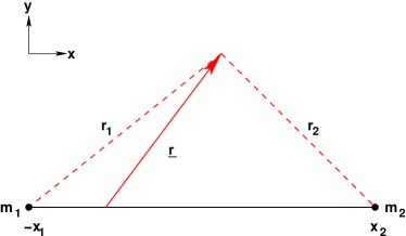
As shown in Figure 37, we consider a binary system in which the massive bodies have mass and respectively. We work in a corotating co-ordinate system centered on the center of mass. The orbital plane is in Cartesian co-ordinates, and the test particle is located at position .
If the angular velocity of the binary is , the equations of motion for the test particle are,
| (280) | |||||
| (281) |
Expressed in components, we have,
| (282) |
The acceleration due to the centrifugal force can be subsumed into a pseudo-potential. Defining,
| (283) |
we obtain,
| (284) |
Digressing briefly, we note that is (up to an arbitrary minus sign) the “Roche potential”. Two stars, or a star plus a planet, that rotate synchronously while on circular orbits occupy Roche equipotentials. If their size is comparable to the size of the Roche lobe—defined by the critical figure-of-eight shaped equipotential that passes through the inner Lagrange point —then the bodies suffer significant tidal distortion. A useful approximation for the radius of a sphere with the same volume as the Roche lobe was provided by Eggleton (1983). For a binary with mass ratio and separation ,
| (285) |
This equation can be used to assess, for example, how close hot Jupiters are to overflowing their Roche lobes. For a Jupiter mass planet with ,
| (286) |
A planet with the same radius as Jupiter ( cm) would then overflow its Roche lobe interior to AU. A very short period hot Jupiter, such as OGLE-TR-56b Torres et al. (2004) with a period of 1.2 days, has a semi-major axis that is about 0.0225 AU. So this planet, and more securely other hot Jupiters that orbit modestly further out, is safe against mass transfer, though not by a large margin.
Returning to the general equations (284), we eliminate the Coriolis terms by multiplying through by , and and adding. We then obtain,
| (287) |
where is the velocity and , called the Jacobi constant, is the arbitrary constant of integration. is an energy-like quantity that is a conserved quantity in the circular restricted 3-body problem.
The existence of this integral of motion is important because it places limits on the range of motion possible for the test particle. For a particle with a given initial position and velocity, we can use equation (287) to compute , and hence to specify zero-velocity surfaces, defined via,
| (288) |
which the particle can never cross. If the volume enclosed by one of the zero-velocity surface is finite, then a particle initially within that region is guaranteed to remain there for all time. This concept is known as Hill stability.
The topology of the zero-velocity surfaces in the restricted three-body problem varies according to the value of . An example is shown in Figure 38. In this instance the zero-velocity surfaces define three disjoint regions in the plane, one corresponding to orbits around the star, one corresponding to orbits around the planet, and one corresponding to orbits around the star-planet binary. A particle in any one of these states is stuck there – it cannot cross the forbidden zone between the different regions to move into a different state.
IV.3.2 Scattering and exoplanet eccentricities
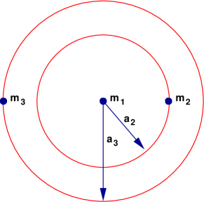
Somewhat surprisingly, the result of the test particle analysis discussed above also applies in modified form to the much tougher problem of the stability of two planets orbiting a star. Consider the situation shown in Figure 39, in which planets of mass and orbit a star of mass in circular orbits with semi-major axes and respectively. The stability of the system evidently must depend upon the relative, rather than the absolute, spacing between the orbits. Accordingly we write,
| (289) |
with being a dimensionless measure of the orbital separation between the planets. We further define and . Then for ,, Gladman (1993), drawing on earlier results derived by Marchal & Bozis (1982) and others, showed that the system is guaranteed to be stable provided that the separation exceeds a critical separation given by,
| (290) |
Note that analytic results leave open the question of whether systems with are actually unstable, all we know is that is sufficient for stability. This condition reduces to the test particle result if , as of course it should212121Note, however, that the analysis for the restricted three-body problem applies for an arbitrary mass ratio of the massive bodies, whereas the result for two planets requires that both be much less massive than the star.. As an example, if we compute the critical separation for planets of the mass of Jupiter and Saturn, we obtain . The actual separation of Jupiter and Saturn in these units is , so an isolated planetary system in which Jupiter and Saturn were on circular orbits would assuredly be stable for all time.
What about more complex systems? It is possible to include non-zero eccentricities into this analysis, but not more planets. For a multiple planet system one might plausibly reason that the system will be unstable if any pair substantially violates the critical two-planet separation for Hill stability. It is also true that the system will generally become more stable as the separations increase (Chambers, Wetherill & Boss, 1996). However, no absolute stability bound is known for any planetary system with .
If a two-planet system is unstable, the possible outcomes of the instability can be divided into four classes:
-
1.
The separation evolves (increases) until the system achieves a state that is stable over the long term.
-
2.
One planet is ejected, while the other remains bound, generally with .
-
3.
The planets physically collide.
-
4.
One planet impacts the star, or is scattered into a short-period orbit for which tidal effects are important.
The last two channels are not possible in a model 3-body problem, in which the planets are represented by point masses, but can occur (especially planet-planet collisions, which become frequent at small radii) in real systems.
The idea that gravitational scattering and planetary ejections might account for the eccentricity of extrasolar planets was proposed as soon as it became clear that extrasolar planets were not typically on circular orbits Rasio & Ford (1996); Weidenschilling & Marzari (1996); Lin & Ida (1997). Quantitative study of such models requires large-scale N-body integrations, first to derive the statistical distribution of outcomes of any given scenario (since the systems are typically chaotic, nothing can be said about any single run), and second to map out the large parameter space that results when one considers different numbers of planets with different initial separations, masses and so forth.
Ford, Havlickova & Rasio (2001) presented a comprehensive study of the dynamics of equal mass two planet systems. The planets were set up on circular orbits close to the stability boundary, and allowed to evolve under purely N-body forces until the system relaxed to a stable state. They found that the predicted fraction of collisions increases sharply for small orbital radii and / or larger planetary radii. For pairs of Jupiter mass and Jupiter radius planets initially located at 5 AU, the most common outcome is two planets (65%), followed by ejections (35%), with collisions (10%) a distant third. If the same pair of planets starts at 1 AU, however, collisions occur roughly 30% of the time. This conclusion is important for studies of extrasolar planet eccentricity, because collisions yield relatively low eccentricities for the merged planet.
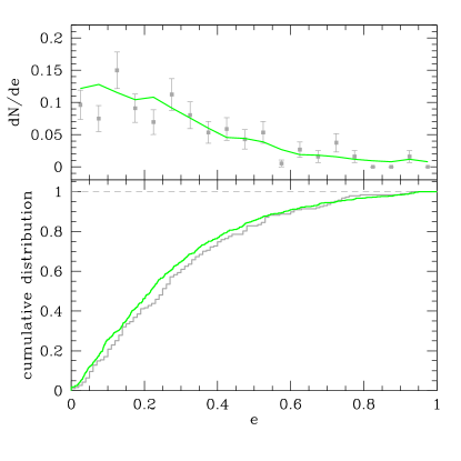
There is only a rather small range of orbital separations which allows a two planet system to be unstable over the long term (greater than around yr, which is roughly the dispersal time for the gas disk), while not being violently unstable. This observation means that it is easier to set up an internally self-consistent scattering model with three or more planets, since a wider range of such systems eventually lead to interesting dynamics. Models starting with three or more planets have also been studied in some detail Terquem & Papaloizou (2002); Marzari & Weidenschilling (2002); Adams & Laughlin (2003). Comprehensive studies, such as those by Chatterjee et al. (2008) and Jurić & Tremaine (2008), find that scattering models yield a good quantitative match to the observed distribution of extrasolar planet eccentricities. Just how good this agreement is is illustrated in Figure 40, which shows how the final simulated eccentricities compare to the data (Raymond et al., 2008). Although these results were derived from purely N-body calculations, hydrodynamic scattering simulations show that the persistence of modest amounts of disk gas does not ruin the agreement (Moeckel & Armitage, 2012). Altogether, there is substantial but circumstantial evidence for a major role for scattering in establishing the broad distribution of exoplanet eccentricity.
IV.4 Predictions of migration theories
In summary, there is persuasive circumstantial evidence for the action of at least three separate processes that lead to the early evolution of planetary systems:
-
•
Gas disk migration in the Type II regime appears to inevitable, since at least some gas must necessarily be present at the epoch when giant planets form. The presence of a reasonably high resonant fraction among systems with multiple giant planets also points to the existence of an early dissipative process in orbital evolution.
-
•
Planetesimal disk migration provides a persuasive explanation for the origin of Pluto’s odd orbit together with some of the more detailed properties of the Kuiper Belt. One can make a case that this process too ought to be common in the outer reaches of planetary systems. Gas giant formation almost certainly becomes more difficult further out in the disk, so it is quite plausible that the zone where gas and ice giants manage to form is often surrounded by a disk of planetesimal debris that has been unable to grow to large sizes.
-
•
Planet-planet scattering works well as an explanation for the eccentricity distribution of giant extrasolar planets. There is no straightforward independent argument that the unstable initial conditions needed for such models to work are generically realized in nature, but the empirical evidence seems to suggest that they are.
The presence of a large fraction of hot Jupiters on orbits inclined with respect to the stellar equator also yields constraints, though these are not unambiguous. Planet-planet scattering (Nagasawa, Ida & Bessho, 2008) or Kozai-Lidov excitation of eccentricity (Wu & Murray, 2003; Naoz, 2016) are the mechanisms most obviously compatible with this observation, but it has also been suggested that the gas disk could be torqued out of the stellar equatorial plane (Bate, Lodato & Pringle, 2010; Batygin, 2012). If this process is common, some or all of the misaligned hot Jupiters could have arrived to their current orbits via Type II migration.
Additional qualitatively different tests of these theoretical ideas are possible. Planet-planet scattering, for example, predicts the existence of a (small) population of very weakly bound, typically eccentric planets, with semi-major axes of AU and more (Veras, Crepp & Ford, 2009; Scharf & Menou, 2009). Direct imaging surveys of young stars have the potential to detect this distinctive population.
The combined action of multiple evolutionary mechanisms may also give rise to new classes of planetary systems. At larger orbital radii (than those currently probed by observations of exoplanets) it seems likely that we ought to see planetary systems whose dynamics has been affected by both planet-planet scattering and planetesimal disk migration. N-body simulations suggest that the signature of this combination is a transition from generally eccentric to nearly circular planetary orbits as the mass of the planetary system is reduced (Raymond, Armitage & Gorelick, 2009, 2010). If true, the near-circular orbits of the giant planets in the Solar System might in fact be typical of the architecture of relatively low-mass systems at large orbital radii. For higher mass systems the same simulations predict a high abundance of resonant configurations, including resonant chains that would be planetary analogs of the Laplace resonance in the Jovian satellite system.
IV.5 Tidal evolution
Two bodies in a tight orbit experience tidal forces as a consequence of the gradient in the gravitational force across their finite radius. The tidal forces raise tidal bulges on the surface of the bodies, whose shape is approximately defined by the condition of hydrostatic equilibrium in the asymmetric gravitational potential. If the axis of the tidal bulge is offset with respect to the line joining the centers of the two bodies, the result is a tidal torque which modifies the semi-major axis and eccentricity of the system.
Tides are dynamically important in the Solar System. Energy dissipation associated with oceanic tides, raised on the Earth by the Moon, is responsible for a slow but measureable increase in the Earth-Moon separation (Dickey et al., 1994). The basic framework for understanding these phenomena dates back to work by George Darwin (Charles’ son) more than a century ago (Darwin, 1879), but even this classical theory involves many subtleties, while a general first-principles theory of tides remains elusive. Ogilvie (2014) gives an excellent review of the state of theoretical knowledge of tidal phenomena.
IV.5.1 The tidal bulge and tidal torque

Even the elementary theory of tides is quite intricate. We can gain considerable physical insight, however, from a simple “back of the envelope” calculation that ignores order unity numerical factors and effects. Consider the tide raised on a fluid body of mass and radius by a companion, of mass , orbiting in a circular orbit at distance . The geometry is shown in Figure 41. We seek to determine, first, the height of the tide , and, second, the torque that results if the tidal bulge is misalinged by some angle with respect to the line joining the centers of the two bodies. We will assume, throughout, that the tidal deformation corresponds closely to the hydrostatic response of the body in the gravitational field defined by both bodies (the “static” tide). This is a reasonable approximation. Applying the virial theorem to the body on which the tide is raised, we find that the central sound speed ought to be comparable to the orbital velocity around the body at radius . For , it follows that one orbit of the companion corresponds to many sound crossing times of the fluid, and hydrostatic equilibrium has time to be established.
To estimate the height of the tidal bulge, , we note that the gravitational force (per unit mass) exerted by the companion on the near side of the body differs from that exerted at the center by an amount,
| (291) |
This tidal force allows us to raise a tidal bulge up to a height where the self-gravity of the fluid body is reduced by the same amount,
| (292) | |||
| (293) |
The height of the bulge falls off rapidly for . If we assume that the fluid body has a uniform density (and thereby ignore important structural factors) the mass associated with the bulge is given by,
| (294) |
which simplifies to yield,
| (295) |
The work required to raise the bulge against the self-gravity of the fluid body is,
| (296) | |||||
| (297) |
This is the amount of energy associated with the tidal deformation of the body.
Let us now backtrack to revisit the assumption that the tidal response of the fluid is hydrostatic. If this were exactly true, the tidal bulge would line up precisely along the line joining the centers of the two bodies, and, by symmetry, there would be no tidal torque (as shown in the upper panel of Figure 41). In reality, however, the tide represents the response of the fluid to forcing at some non-zero frequency , given (for a companion on a circular orbit around a non-rotating primary) simply by the orbital frequency. If the central body is non-rotating (or rotating slower than the orbital frequency), then the departure from hydrostatic equilibrium occasioned by the finite response time will cause the bulge to lag by some angle . The bulge will lead if the spin of the central body is faster than the orbital frequency. A lagging or leading bulge will exert a torque on the companion that causes the orbit to decay or expand in radius, respectively (e.g. the Moon’s orbital period exceeds the Earth’s spin period, so the torque for the Earth-Moon system results in recession of the lunar orbit away from the Earth).
We now assume that the torque due to the tide can be represented as that due to two point masses offset from the line of centers by a small angle (Figure 41, lower diagram). The tidal force is then, roughly,
| (298) | |||||
| (299) |
and the work done by the tidal force per orbit of the companion is,
| (300) |
If we knew , this equation (with the missing numerical factors restored) would yield the rate of decay or rate of expansion of the orbit due to the tides.
Calculating from first principles is a hard task. We can, however, at least gain a more transparent understanding of the physical problem of what determines . To do so we define the tidal as the ratio of the energy stored in the tidal deformation to the energy that is dissipated in one cycle,
| (301) |
Using our estimates, we have that,
| (302) |
This is an important result. We see that the magnitude of the tidal lag, and hence the strength of the tidal torque, is directly linked to the amount of dissipation within the tidally distorted body.
Finally we can estimate the rate of decay of the orbital separation due to the (lagging) tidal bulge. For we have that,
| (303) |
where is the orbital period. Substituting for the various quantities, we obtain,
| (304) |
Up to factors of the order of unity, this expression agrees with the standard tidal formula quoted, for example, by Jackson, Greenberg & Barnes (2008), who also give the corresponding expressions for the change in orbital eccentricity. Standard references for the astrophysical theory of tides include Goldreich & Soter (1966) and Hut (1981).
IV.5.2 Determining the tidal
The above analysis suffices to illustrate two important points,
-
•
Tidal forces decline extremely rapidly with increasing orbital separation.
-
•
The rate of tidal evolution depends upon the amount of dissipation present within the two bodies that are interacting tidally.
The attentive reader may also have noticed the astrophysical sleight of hand by which all manner of intractable physics has been swept into a single unknown parameter, . Approaches to estimating can be divided into those that rely on extrapolations from measured values in well-observed systems, and those that attempt to compute by identifying dissipative processes within stars or planets.
For giant planets, the primary observational constraint on comes from direct measurements of the tidal evolution in the orbits of the Galilean satellites (Yoder & Peale, 1981; Lainey et al., 2009)222222Historically, estimates of Jupiter’s have primarily been derived indirectly, by assuming that the excess heat flux from Io derives from tidal effects. Greenberg (2010) gives a good review of these estimates.. These empirical estimates suggest that , and based on this many workers adopt values for the tidal of extrasolar planets that are similar (typically in the range ). Considerable caution as to the validity of this extrapolation from Jupiter to extrasolar planets is, however, in order. As noted already, the of a star or planet is not some fixed and immutable property of a body akin, say, to its mass. Rather, describes the response of a body to forcing at one or more specific frequencies (in the case of the Jovian estimate, the frequency of relevance is the difference between the spin frequency of Jupiter and the orbital frequency of Io). To extrapolate correctly to extrasolar planets, we need to make some assumption as to how varies as a function of frequency. One simple assumption is to postulate that the tidal lag angle remains constant—in which case is indeed a constant—but one might equally assume that the tidal bulge has a constant time lag, in which case . If one is interested in tidal eccentricity evolution, moreover, the forcing is not monochromatic but rather has a spread across a range of frequencies. As a result of these complications, empirical models of extrasolar tidal evolution are subject to substantial but unquantifiable uncertainties.
Given the uncertainties in the empirical approach, a theoretical determination of would evidently be extremely valuable. Achieving this goal requires first identifying, and then calculating, the primary source of dissipation that acts on the tide. Molecular viscosity is insufficient, so we are left with a variety of hard-to-calculate candidates that include non-linear dissipation of waves and interactions between the tide and turbulent processes within the body. Recent theoretical work (Ogilvie & Lin, 2004; Goodman & Lackner, 2009) in this area, although it still falls short of being able to predict from first-principles, has nonetheless proven influential in identifying additional properties of planets that may influence the . The presence of a rigid, solid core, for example, can substantially alter the tidal response of a planet as compared to an observationally almost indistinguishable body lacking a core. Given the rapidly improving observations of extrasolar planets that are surely vulnerable to tidal evolution, one may hope that this is an area ripe for further theoretical and observational progress.
Acknowledgements
These notes are based on a graduate course given at the University of Colorado, Boulder. My thanks to the students in those classes, and to my current and former postdoctoral collaborators, for stimulating my interest in this subject. My work on planet formation and accretion physics has been supported by NASA under the auspices of the Origins of Solar Systems, Exoplanet Research, Astrophysics Theory, Beyond Einstein Foundation Science and Hubble Theory programs, and by the National Science Foundation.
References
- Adams (2010) Adams, F. C. 2010, ARA&A, 48, 47
- Adams, Lada & Shu (1987) Adams, F. C., Lada, C. J., & Shu, F. H. 1987, ApJ, 312, 788
- Adams & Laughlin (2003) Adams, F. C., & Laughlin, G. 2003, Icarus, 163, 290
- Adams et al. (2006) Adams, F. C., Proszkow, E. M., Fatuzzo, M., & Myers, P. C. 2006, ApJ, 641, 504
- Adams & Shu (1986) Adams, F. C., & Shu, F. H. 1986, ApJ, 308, 836
- Afshordi, Mukhopadhyay & Narayan (2005) Afshordi, N., Mukhopadhyay, B., & Narayan, R. 2005, ApJ, 629, 373
- Agol et al. (2005) Agol, E., Steffen, J., Sari, R., & Clarkson, W. 2005, MNRAS, 359, 567
- Agnor & Hamilton (2006) Agnor, C. B., & Hamilton, D. P. 2006, Nature, 441, 192
- Alexander & Armitage (2007) Alexander, R. D., & Armitage, P. J. 2007, MNRAS, 375, 500
- Alexander & Armitage (2009) Alexander, R. D., & Armitage, P. J. 2009, ApJ, 704, 989
- Alexander, Clarke & Pringle (2005) Alexander, R. D., Clarke, C. J., & Pringle, J. E. 2005, MNRAS, 358, 283
- Alexander, Clarke & Pringle (2006) Alexander, R. D., Clarke, C. J., & Pringle, J. E. 2006, MNRAS, 369, 229
- Alexander et al. (2014) Alexander, R., Pascucci, I., Andrews, S., Armitage, P., & Cieza, L. 2014, Protostars & Planets VI, Henrik Beuther, Ralf S. Klessen, Cornelis P. Dullemond, and Thomas Henning (eds.), University of Arizona Press, Tucson, p. 475
- Alibert et al. (2005) Alibert, Y., Mordasini, C., Benz, W., & Winisdoerffer, C. 2005, A&A, 434, 343
- Andrews et al. (2009) Andrews, S. M., Wilner, D. J., Hughes, A. M., Qi, Chunhua, & Dullemond, C. P. 2009, ApJ, 700, 1502
- Arakawa, Leliwa-Kopystynski & Maeno (2002) Arakawa, M., Leliwa-Kopystynski, J., & Maeno, N. 2002, Icarus, 158, 516
- Armitage (2002) Armitage, P. J. 2002, MNRAS, 330, 895
- Armitage (2010) Armitage, P. J. 2010, Astrophysics of Planet Formation, Cambridge University Press (Cambridge: UK)
- Armitage (2011) Armitage, P. J. 2011, ARA&A, 49, 195
- Armitage (2015) Armitage, P. J. 2015, to appear in From Protoplanetary Disks to Planet Formation, proceedings of the 45th Saas-Fee Advanced Course (arXiv:1509.06382)
- Armitage & Clarke (1996) Armitage, P. J., & Clarke, C. J. 1996, MNRAS, 280, 458
- Armitage, Livio & Pringle (2001) Armitage, P. J., Livio, M., & Pringle, J. E. 2001, MNRAS, 324, 705
- Armitage, Simon & Martin (2013) Armitage, P. J., Simon, J. B., & Martin, R. G. 2013, ApJ, 778, article id. L14
- Armitage & Rice (2005) Armitage, P. J., & Rice, W. K. M. 2005, in A Decade Of Extrasolar Planets Around Normal Stars, STScI May Symposium 2005, astro-ph/0507492
- Artymowicz (1993) Artymowicz, P. 1993, ApJ, 419, 155
- Artymowicz et al. (1991) Artymowicz, P., Clarke, C. J., Lubow, S. H., & Pringle, J. E. 1991, ApJ, 370, L35
- Bai (2014) Bai, X.-N. 2014, ApJ, 791, article id. 137
- Bai (2016) Bai, X.-N. 2016, ApJ, 821, article id. 80
- Bai & Stone (2011) Bai, X.-N., & Stone, J. M. 2011, ApJ, 736, article id. 144
- Bai & Stone (2013) Bai, X.-N., & Stone, J. M. 2013, ApJ, 769, article id. 76
- Bai et al. (2016) Bai, X.-N., Ye, J., Goodman, J., & Yuan, F. 2016, ApJ, 818, article id. 152
- Balbus (2011) Balbus, S. A. 2011, Physical Processes in Circumstellar Disks Around Young Stars, ed. Paulo J.V. Garcia, University of Chicago Press, p. 237 (arXiv:0906.0854)
- Balbus & Hawley (1991) Balbus, S. A., & Hawley, J. F. 1991, ApJ, 376, 214
- Balbus & Hawley (1998) Balbus, S. A., & Hawley, J. F. 1998, Reviews of Modern Physics, 70, 1
- Balbus & Hawley (2006) Balbus, S. A., & Hawley, J. F. 2006, ApJ, 652, 1020
- Balbus, Hawley & Stone (1996) Balbus, S. A., Hawley, J. F., & Stone, J. M. 1996, ApJ, 467, 76
- Balbus & Terquem (2001) Balbus S. A., & Terquem C. 2001, ApJ, 552, 235
- Bally & Scoville (1982) Bally, J., & Scoville, N. Z. 1982, ApJ, 255, 497
- Barge & Sommeria (1995) Barge, P., & Sommeria, J. 1995, A&A, 295, L1
- Barranco & Marcus (2005) Barranco, J. A., & Marcus, P. S. 2005, ApJ, 623, 1157
- Baruteau et al. (2014) Baruteau, C., et al. 2014, Protostars & Planets VI, Henrik Beuther, Ralf S. Klessen, Cornelis P. Dullemond, and Thomas Henning (eds.), University of Arizona Press, Tucson, p. 667
- Basri, Walkowicz & Reiners (2012) Basri, G., Walkowicz, L. M., & Reiners, A. 2013, ApJ, 769, article id. 37
- Bate, Lodato & Pringle (2010) Bate, M. R., Lodato, G., & Pringle, J. E. 2010, MNRAS, 401, 1505
- Batygin (2012) Batygin, K. 2012, Nature, 491, 418
- Batygin (2015) Batygin, K. 2015, MNRAS, 451, 2589
- Batygin & Adams (2017) Batygin, K., & Adams, F. C. 2017, AJ, in press (arXiv:1701.07849)
- Batygin & Brown (2010) Batygin, K., & Brown, M. E. 2010, ApJ, 716, 1323
- Batygin & Brown (2016) Batygin, K., & Brown, M. E. 2016, AJ, 151, article id. 22
- Batygin, Brown & Fraser (2011) Batygin, K., Brown, M. E., & Fraser, W. C. 2011, ApJ, 738, 13
- Batygin & Stevenson (2010) Batygin, K., & Stevenson, D. J. 2010, ApJ, 714, L238
- Beaulieu et al. (2006) Beaulieu, J.-P., et al. 2006, Nature, 439, 437
- Begelman, McKee & Shields (1983) Begelman, M. C., McKee, C. F., & Shields, G. A. 1983, ApJ, 271, 70
- Bell et al. (1997) Bell, K. R., Cassen, P. M., Klahr, H. H., & Henning, Th. 1997, ApJ, 486, 372
- Bell & Lin (1994) Bell, K. R., & Lin, D. N. C. 1994, ApJ, 427, 987
- Belyaev, Rafikov & Stone (2013) Belyaev, M. A., Rafikov, R. R., & Stone, J. M. 2013, ApJ, 770, article id. 68
- Benz & Asphaug (1999) Benz, W., & Asphaug, E. 1999, Icarus, 142, 5
- Benz, Slattery & Cameron (1986) Benz, W., Slattery, W. L., & Cameron, A. G. W. 1986, Icarus, 66, 515
- Béthune, Lesur & Ferreira (2017) Béthune, W., Lesur, G., & Ferreira, J. 2017, A&A, in press (arXiv:1612.00883)
- Binney & Tremaine (1987) Binney, J., & Tremaine, S. 1987, Galactic Dynamics, Princeton University Press, p. 310
- Birnstiel, Klahr & Ercolano (2012) Birnstiel, T., Klahr, H., & Ercolano, B. 2012, A&A, 539, id. A148
- Birnstiel, Ormel & Dullemond (2011) Birnstiel, T., Ormel, C. W., & Dullemond, C. P. 2011, A&A, 525, id. A11
- Bitsch et al. (2013) Bitsch, B., Crida, A., Morbidelli, A., Kley, W., & Dobbs-Dixon, I. 2013, A&A, 549, id. A124
- Bitsch, Lambrechts & Johansen (2015) Bitsch, B., Lambrechts, M., & Johansen, A. 2015, A&A, 582, id. A112
- Blaes & Balbus (1994) Blaes, O. M., & Balbus, S. A. 1994, ApJ, 421, 163
- Blandford & Payne (1982) Blandford, R. D., & Payne, D. G. 1982, MNRAS, 199, 883
- Blum & Wurm (2008) Blum, J., & Wurm, G. 2008, ARA&A, 46, 21
- Bodenheimer & Pollack (1986) Bodenheimer, P., & Pollack, J. B. 1986, Icarus, 67, 391
- Boley et al. (2009) Boley, A. C. 2009, ApJ, 695, L53
- Boley et al. (2010) Boley, A. C., Hayfield, T., Mayer, L., & Durisen, R. H. 2010, Icarus, 207, 509
- Boss (1997) Boss, A. P. 1997, Science, 276, 1836
- Bouvier et al. (2007) Bouvier, J., Alencar, S. H. P., Harries, T. J., Johns-Krull, C. M., & Romanova, M. M. 2007, Protostars and Planets V, eds B. Reipurth, D. Jewitt, and K. Keil, University of Arizona Press, Tucson, astro-ph/0603498
- Brandenburg et al. (1995) Brandenburg, A.,, Nordlund, A., Stein, R. F., & Torkelsson, U. 1995, ApJ, 446, 741
- Bromley & Kenyon (2006) Bromley, B. C., & Kenyon, S. J. 2006, AJ, 131, 2737
- Brown, Trujillo & Rabinowitz (2004) Brown, M. E., Trujillo, C., & Rabinowitz, D. 2004, ApJ, 617, 645
- e.g. Burrows et al. (1996) Burrows, C. J., et al. 1996, ApJ, 473, 437
- Burrows et al. (2007) Burrows, A., Hubeny, I, Budaj, J., & Hubbard, W. B. 2007, ApJ, 661, 502
- Butler et al. (1996) Butler, R. P., Marcy, G. W., Williams, E., McCarthy, C., Dosanjh, P., & Vogt, S. S. 1996, PASP, 108, 500
- Calvet et al. (2005) Calvet, N., et al. 2005, ApJ, 630, L185
- Cameron (1978) Cameron, A. G. W. 1978, Moon and the Planets, 18, 5
- Cannizzo (1993) Cannizzo, J. K. 1993, ApJ, 419, 318
- Canup (2004) Canup, R. M. 2004, ARA&A, 42, 441
- Canup (2012) Canup, R. M. 2012, Science, 338, 1052
- Canup & Ward (2002) Canup, R. M., & Ward, W. R. 2002, AJ, 124, 3404
- Canup & Ward (2008) Canup, R. M., & Ward, W. R. 2009, in Europa, Edited by Robert T. Pappalardo, William B. McKinnon, Krishan K. Khurana. University of Arizona Press, Tucson, p. 59
- Carlberg & Sellwood (1985) Carlberg, R. G., & Sellwood, J. A. 1985. ApJ, 292, 79
- Carrera, Johansen & Davies (2015) Carrera, D., Johansen, A., & Davies, M. B. 2015, A&A, 579, id. A43
- Carter et al. (2012) Carter, J. A., et al. 2012, Science, 337, 556
- Casoli & Masset (2009) Casoli, J., & Masset, F. S. 2009, ApJ, 703, 845
- Chambers (2014) Chambers, J. E. 2014, Icarus, 233, 83
- Chambers & Wetherill (1998) Chambers, J. E., & Wetherill, G. W. 1998, Icarus, 136, 304
- Chambers, Wetherill & Boss (1996) Chambers, J. E., Wetherill, G. W., & Boss, A. P. 2006, Icarus, 119, 261
- Chandrasekhar (1961) Chandrasekhar, S. 1961, Hydrodynamic and hydromagnetic stability, International Series of Monographs on Physics, Oxford: Clarendon
- Chapman & Cowling (1970) Chapman, S., & Cowling, T. G. 1970, The mathematical theory of non-uniform gases, Cambridge University Press
- Charbonneau et al. (2009) Charbonneau, D., et al. 2009, Nature, 462, 891
- Chatterjee & Ford (2015) Chatterjee, S., & Ford, E. B. 2015, ApJ, 803, article id. 33
- Chatterjee et al. (2008) Chatterjee, S., Ford, E. B., Matsumura, S., & Rasio, F. A. 2008, ApJ, 686, 580
- Chiang & Goldreich (1997) Chiang, E. I., & Goldreich, P. 1997, ApJ, 490, 368
- Chiang et al. (2007) Chiang, E., Lithwick, Y., Murray-Clay, R., Buie, M., Grundy, W., & Holman, M. 2007, Protostars and Planets V, eds B. Reipurth, D. Jewitt, and K. Keil, University of Arizona Press, Tucson, astro-ph/0601654
- Clarke (2009) Clarke, C. J. 2009, MNRAS, 396, 1066
- Clarke, Gendrin & Sotomayor (2001) Clarke, C. J., Gendrin, A., & Sotomayor, M. 2001, MNRAS, 328, 485
- Cleeves et al. (2015) Cleeves, L. I., Bergin, E. A., Qi, C., Adams, F. C., & Öberg, K. I. 2015, ApJ, 799, article id. 204
- Cleeves et al. (2016) Cleeves, L. I., Öberg, K. I., Wilner, D. J., Huang, J., Loomis, R. A., Andrews, S. M., & Czekala, I. 2016, ApJ, 832, article id. 110
- Coleman & Nelson (2016) Coleman, G. A. L., & Nelson, R. P. 2016, MNRAS, 457, 2480
- Collier Cameron & Campbell (1993) Collier Cameron, A., & Campbell, C. G. 1993, A&A, 274, 309
- Ćuk & Stewart (2012) Ćuk, M., & Stewart, S. T. 2012, Science, 338, 1047
- Ćuk et al. (2016) Ćuk, M., Hamilton, D. P., Lock, S. J., & Stewart, S. T. 2016, Nature, 539, 402
- Cumming et al. (2008) Cumming, A., et al. 2008, PASP, 120, 531
- Cuzzi, Dobrovolskis & Champney (1993) Cuzzi, J. N., Dobrovolskis, A. R., & Champney, J. M. 1993, Icarus, 106, 102
- Cuzzi, Hogan & Shariff (2008) Cuzzi, J. N., Hogan, R. C., & Shariff, K. 2008, ApJ, 687, 1432
- D’Angelo, Lubow & Bate (2006) D’Angelo, G., Lubow, S. H., & Bate, M. R. 2006, ApJ, 652, 1698
- Darwin (1879) Darwin, G. H. 1879, Philos. Trans. of Roy. Soc., 170, 447
- Davies et al. (2014) Davies, M. B., Adams, F. C., Armitage, P., Chambers, J., Ford, E., Morbidelli, A., Raymond, S. N., & Veras, D. 2014, to appear in in Protostars & Planets VI, eds. H. Beuther, C. Dullemond, Th. Henning, R. Klessen, University of Arizona Press
- Davis, Stone & Pessah (2010) Davis, S. W., Stone, J. M., & Pessah, M. E. 2010, ApJ, 713, 52
- Dawson & Murray-Clay (2012) Dawson, R. I., & Murray-Clay, R. 2012, ApJ, 750, 43
- Deienno et al. (2017) Deienno, R., Morbidelli, A., Gomes, R. S., & Nesvorny, D. 2017, AJ, in press (arXiv:1702.02094)
- Demory & Seager (2011) Demory, B.-O., & Seager, S. 2011, ApJS, 197, article id. 12
- Desch (2004) Desch, S. J. 2004, ApJ, 608, 509
- Dickey et al. (1994) Dickey, J. O., et al. 1994, Science, 265, 482
- Doyle et al. (2011) Doyle, L. R., et al. 2011, Science, 333, 1602
- Dubrulle, Morfill & Sterzik (1995) Dubrulle, B., Morfill, G., & Sterzik, M. 1995, Icarus, 114, 237
- Duffell et al. (2014) Duffell, P. C., Haiman, Z., MacFadyen, A. I., D’Orazio, D. J., & Farris, B. D. 2014, ApJ, 792, article id. L10
- Duffell & Chiang (2015) Duffell, P. C., & Chiang, E. 2015, ApJ, 812, article id. 94
- Dullemond & Dominik (2005) Dullemond, C. P., & Dominik, C. 2005, A&A, 434, 971
- Dullemond et al. (2007) Dullemond, C. P., Hollenbach, D., Kamp, I., & D’Alessio, P. 2007, Protostars and Planets V, eds B. Reipurth, D. Jewitt, and K. Keil, University of Arizona Press, Tucson, astro-ph/0602619
- Dunhill, Alexander & Armitage (2013) Dunhill, A. C.; Alexander, R. D., & Armitage, P. J. 2013, MNRAS, 428, 3072
- Durisen et al. (2005) Durisen, R. H., Cai, K., Mejía, A. C., & Pickett, M. K. 2005, Icarus, 173, 417
- Dürmann & Kley (2015) Dürmann, C., & Kley, W. 2015, A&A, 574, id. A52
- Dürmann & Kley (2017) Dürmann, C., & Kley, W. 2017, A&A, 598, id. A80
- Eggleton (1983) Eggleton, P. P. 1983, ApJ, 268, 368
- Eisner, Chiang & Hillenbrand (2006) Eisner, J. A., Chiang, E. I., & Hillenbrand, L. A. 2006, ApJ, 637, L133
- Eisner et al. (2005) Eisner, J. A., Hillenbrand, L. A., Carpenter, J. M., & Wolf, S. 2005, ApJ, 635, 396
- Elser et al. (2011) Elser, S., Moore, B., Stadel, J., & Morishima, R. 2011, Icarus, 214, 357
- Ercolano, Clarke & Drake (2009) Ercolano, B., Clarke, C. J., & Drake, J. J. 2009, ApJ, 699, 1639
- Ercolano & Glassgold (2013) Ercolano, B., & Glassgold, A. E. 2013, MNRAS, 436, 3446
- Espaillat et al. (2014) Espaillat, C., et al. 2014, Protostars and Planets VI, Henrik Beuther, Ralf S. Klessen, Cornelis P. Dullemond, and Thomas Henning (eds.), University of Arizona Press, Tucson, p. 497
- Estrada et al. (2009) Estrada, P. R., Mosqueira, I., Lissauer, J. J., D’Angelo, G., & Cruikshank, D. P. 2009, in Europa, Edited by Robert T. Pappalardo, William B. McKinnon, Krishan K. Khurana. University of Arizona Press, Tucson, p. 27
- Evans & Tabachnik (1999) Evans, N. W., & Tabachnik, S. 1999, Nature, 399, 41
- Everett et al. (2013) Everett, M. E., Howell, S. B., Silva, D. R., & Szkody, P. 2013, ApJ, 771, article id. 107
- Fabian, Pringle & Rees (1975) Fabian, A. C., Pringle, J. E., & Rees, M. J. 1975, MNRAS, 172, 15
- Fabrycky et al. (2014) Fabrycky, D. C., et al. 2014, ApJ, 790, article id. 146
- Feigelson et al. (2007) Feigelson, E., Townsley, L., Güdel, M., & Stassun, K. 2007, Protostars and Planets V, eds B. Reipurth, D. Jewitt, and K. Keil, University of Arizona Press, Tucson, p. 313
- Fernandez & Ip (1984) Fernandez, J. A., & Ip, W.-H. 1984, Icarus, 58, 109
- Fienga et al. (2016) Fienga, A., Laskar, J., Manche, H., & Gastineau, M. 2016, A&A, 587, id. L8
- Fischer & Valenti (2005) Fischer, D. A., & Valenti, J. 2005, ApJ, 622, 1102
- Flaherty et al. (2015) Flaherty, K. M., Hughes, A. M., Rosenfeld, K. A., Andrews, S. M., Chiang, E., Simon, J. B., Kerzner, S., & Wilner, D. J. 2015, ApJ, 813, article id. 99
- Font et al. (2004) Font, A. S., McCarthy, I. G., Johnstone, D., & Ballantyne, D. R. 2004, ApJ, 607, 890
- Ford, Havlickova & Rasio (2001) Ford, E. B., Havlickova, M., & Rasio, F. A. 2001, Icarus, 150, 303
- Ford et al. (2012) Ford, E. B., et al. 2012, ApJ, 756, article id. 185
- Forgan, Price & Bonnell (2017) Forgan, D., Price, D. J., & Bonnell, I. 2017, MNRAS, 466, 3406
- Frank, King & Raine (2002) Frank, J., King, A., & Raine, D. J. 2002, Accretion Power in Astrophysics, (3rd edition, Cambridge University Press)
- Fraser et al. (2014) Fraser, W. C., Brown, M. E., Morbidelli, A., Parker, A., & Batygin, K. 2014, ApJ, 782, 100
- Fraser & Kavelaars (2009) Fraser, W. C., & Kavelaars, J. J. 2009, AJ, 137, 71
- Fricke (1968) Fricke, K. 1968, Zeitschrift für Astrophysik, 68, 317
- Fromang & Papaloizou (2006) Fromang, S., & Papaloizou, J. 2006, A&A, 452, 751
- Galicher (2016) Galicher, R., et al. 2016, A&A, 594, id. A63
- Gammie (1996) Gammie, C. F. 1996, ApJ, 457, 355
- Gammie (2001) Gammie, C. F. 2001, ApJ, 553, 174
- Garaud & Lin (2007) Garaud, P., & Lin, D. N. C. 2007, ApJ, 654, 606
- Gaudi (2010) Gaudi, B. S. 2010, in Exoplanets, ed. S. Seager, University of Arizona Press (arXiv:1002.0332)
- Gilliland et al. (2012) Gilliland, R. L., et al. 2012, ApJ, 197, article id. 6
- Ginsburg & Sari (2016) Ginzburg, S., & Sari, R. 2016, ApJ, 819, 116
- Gladman (1993) Gladman, B. 1993, Icarus, 106, 247
- Godon & Livio (1999) Godon, P., & Livio, M. 1999, ApJ, 523, 350
- Goldreich (1965) Goldreich, P. 1965, MNRAS, 130, 159
- Goldreich, Lithwick & Sari (2004) Goldreich, P., Lithwick, Y., & Sari, R. 2004, ARA&A, 42, 549
- Goldreich & Sari (2003) Goldreich, P., & Sari, R. 2003, ApJ, 585, 1024
- Goldreich & Schlichting (2014) Goldreich, P., & Schlichting, H. E. 2014, AJ, 147, article id. 32
- Goldreich & Schubert (1967) Goldreich, P., & Schubert, G. 1967, ApJ, 150, 571
- Goldreich & Soter (1966) Goldreich, P., & Soter, S. 1966, Icarus, 5, 375
- Goldreich & Tremaine (1979) Goldreich, P., & Tremaine, S. 1979, ApJ, 233, 857
- Goldreich & Tremaine (1980) Goldreich, P., & Tremaine, S. 1980, ApJ, 241, 425
- Goldreich & Ward (1973) Goldreich, P., & Ward, W. R. 1973, ApJ, 183, 1051
- Gomes et al. (2005) Gomes, R., Levison, H. F., Tsiganis, K., & Morbidelli, A. 2005, Nature, 435, 466
- Gomez & Ostriker (2005) Gómez, G. C., & Ostriker, E. C. 2005, ApJ, 630, 1093
- Goodman & Lackner (2009) Goodman, J., & Lackner, C. 2009, ApJ, 696, 2054
- Gorti & Hollenbach (2009) Gorti, U., & Hollenbach, D. 2009, ApJ, 690, 1539
- Greenberg (2010) Greenberg, R. 2010, Reports on Progress in Physics, 73, 036801
- Gressel et al. (2015) Gressel, O., Turner, N. J., Nelson, R. P., & McNally, C. P. 2015, ApJ, 801, article id. 84
- Güdel et al. (2014) Güdel, M., et al. 2014, Protostars and Planets VI, Henrik Beuther, Ralf S. Klessen, Cornelis P. Dullemond, and Thomas Henning (eds.), University of Arizona Press, Tucson, p. 883
- Guillot (2005) Guillot, T. 2005, Annual Review of Earth and Planetary Sciences, 33, 493
- Guillot & Showman (2002) Guillot, T., & Showman, A. P. 2002, A&A, 385, 156
- Gullbring et al. (1998) Gullbring, E., Hartmann, L., Briceno, C., & Calvet, N. 1998, ApJ, 492, 323
- Gundlach & Blum (2015) Gundlach, B., & Blum, J. 2015, ApJ, 798, article id. 34
- Güttler et al. (2010) Güttler, C., Blum, J., Zsom, A., Ormel, C. W., & Dullemond, C. P. 2010, A&A, 513, 56
- Hahn & Malhotra (2005) Hahn, J. M., & Malhotra, R. 2005, AJ, 130, 2392
- Haisch, Lada & Lada (2001) Haisch, K. E., Lada, E. A., & Lada, C. J. 2001, ApJ, 553, L153
- Hands, Alexander & Dehnen (2014) Hands, T. O., Alexander, R. D., & Dehnen, W. 2014, MNRAS, 445, 749
- Hansen (2009) Hansen, B. M. S. 2009, ApJ, 703, 1131
- Hansen (2010) Hansen, B. M. S. 2010, ApJ, 723, 285
- Hartman et al. (2014) Hartman, J. D., et al. 2014, AJ, 147, article id. 128
- Hartmann et al. (1998) Hartmann, L., Calvet, N., Gullbring, E., & D’Alessio, P. 1998, ApJ, 495, 385
- Hartmann & Davis (1975) Hartmann, W. K., & Davis, D. R. 1975, Icarus, 24, 504
- Hartmann & Kenyon (1995) Hartmann, L., & Kenyon, S. J. 1995, ARA&A, 34, 207
- Hayashi (1981) Hayashi, C. 1981, Progress of Theoretical Physics Supplement, 70, 35
- Herbst & Mundt (2005) Herbst, W., & Mundt, R. 2005, ApJ, 633, 967
- Hirose & Turner (2011) Hirose, S., & Turner, N. J. 2011, ApJ, 732, article id. L30
- Hollenbach et al. (1994) Hollenbach, D., Johnstone, D., Lizano, S., & Shu, F. 1994, ApJ, 428, 654
- Holman & Murray (2005) Holman, M. J., & Murray, N. W. 2005, Science, 307, 1288
- Holman & Wisdom (1993) Holman, M. J., & Wisdom, J. 1993, AJ, 105, 1987
- Howard et al. (2012) Howard, A. W., et al. 2012, ApJS, 201, article id. 15
- Hubickyj, Bodenheimer & Lissauer (2005) Hubickyj, O., Bodenheimer, P., & Lissauer, J. J. 2005, Icarus, 179, 415
- Hut (1981) Hut, P. 1981, A&A, 99, 126
- Ida et al. (2000) Ida, S., Bryden, G., Lin, D. N. C., & Tanaka, H. 2000, ApJ, 534, 428
- Ida, Guillot & Morbidelli (2008) Ida, S., Guillot, T., & Morbidelli, A. 2008, ApJ, 686, 1292
- Ida & Lin (2004) Ida, S., Lin, D. N. C. 2004, ApJ, 616, 567
- Ikoma, Nakazawa & Emori (2000) Ikoma, M., Nakazawa, K., & Emori, H. 2000, ApJ, 537, 1013
- Ioannou & Kakouris (2001) Ioannou, P. J., & Kakouris, A. 2001, ApJ, 550, 931
- Inaba et al. (2001) Inaba, S., Tanaka, H., Nakazawa, K., Wetherill, G. W., & Kokubo, E. 2001, Icarus, 149, 235
- Ivanov, Papaloizou & Polnarev (1999) Ivanov, P. B., Papaloizou, J. C. B., & Polnarev, A. G. 1999, MNRAS, 307, 79
- Jackson, Greenberg & Barnes (2008) Jackson, B., Greenberg, R., & Barnes, R. 2008, ApJ, 678, 1396
- Jewitt & Haghighipour (2007) Jewitt, D., & Haghighipour, N. 2003, ARA&A, 45, 261
- Jewitt & Luu (1993) Jewitt, D., & Luu, J. 1993, Nature, 362, 730
- Ji et al. (2006) Ji, H., Burin, M., Schartman, E., & Goodman, J. 2006, Nature, 444, 343
- Johansen, Henning & Klahr (2006) Johansen, A., Henning, T., & Klahr, H. 2006, ApJ, 643, 1219
- Johansen et al. (2007) Johansen, A., Oishi, J. S., Mac Low, M.-M., Klahr, H., Henning, T., & Youdin, A. 2007, Nature, 448, 1022
- Johansen, Youdin & Klahr (2009b) Johansen, A., Youdin, A., & Klahr, H. 2009, ApJ, 697, 1269
- Johansen, Youdin & Mac Low (2009) Johansen, A., Youdin, A., & Mac Low, M.-M. 2009, ApJ, 704, L75
- Johnson & Gammie (2005) Johnson, B. M., & Gammie, C. F. 2005, ApJ, 635, 149
- Johnstone, Hollenbach & Bally (1998) Johnstone, D., Hollenbach, D., & Bally, J. 1998, ApJ, 499, 758
- Jurić & Tremaine (2008) Jurić, M., & Tremaine, S. 2008, ApJ, 686, 603
- Kaib & Chambers (2016) Kaib, N. A., & Chambers, J. E. 2016, MNRAS, 455, 3561
- Kasting, Whitmire & Reynolds (1993) Kasting, J. F., Whitmire, D. P., & Reynolds, R. T. 1993, Icarus, 101, 108
- Kenyon & Hartmann (1987) Kenyon, S. J., & Hartmann, L. 1987, ApJ, 323, 714
- Kenyon & Luu (1998) Kenyon, S. J., & Luu, J. X. 1998, AJ, 115, 2136
- King, Pringle & Livio (2007) King, A. R., Pringle, J. E., & Livio, M. 2007, MNRAS, 376, 1740
- Kirsh et al. (2009) Kirsh, D. R., Duncan, M., Brasser, R., & Levison, H. F. 2009, Icarus, 199, 197
- Klahr & Bodenheimer (2003) Klahr, H. H., & Bodenheimer, P. 2003, ApJ, 582, 869
- Kley, Bitsch & Klahr (2009) Kley, W., Bitsch, B., & Klahr, H. 2009, A&A, 506, 971
- Kley & Crida (2008) Kley, W., & Crida, A. 2008, A&A, 487, L9
- Kley & Nelson (2012) Kley, W., & Nelson, R. P. 2012, ARA&A, 50, 211
- Kobayashi et al. (2012) Kobayashi, S., Hainick, Y., Sari, R., & Rossi, E. M. 2012, ApJ, 748, 105
- Kokubo & Ida (1998) Kokubo, E., & Ida, S. 1998, Icarus, 131, 171
- Kokubo, Ida & Makino (2000) Kokubo, E., Ida, S., & Makino, J. 2000, Icarus, 148, 419
- Kokubo, Kominami & Ida (2006) Kokubo, E., Kominami, J., & Ida, S. 2006, ApJ, 642, 1131
- Königl (1991) Königl, A. 1991, ApJ, 370, L39
- Königl & Salmeron (2011) Königl, A., & Salmeron, R. 2011, Physical Processes in Circumstellar Disks around Young Stars, ed. Paulo J.V. Garcia, University of Chicago Press, p. 283
- Kopparapu et al. (2013) Kopparapu, R. K., et al. 2013, ApJ, 765, article id. 131
- Kopparapu et al. (2014) Kopparapu, R. K., Ramirez, R. M., SchottelKotte, J., Kasting, J. F., Domagal-Goldman, S., & Eymet, V. 2014, ApJL, 787, article id. L29
- Korycansky & Asphaug (2006) Korycansky, D. G., & Asphaug, E. 2006, Icarus, 181, 605
- Kozai (1962) Kozai, Y. 1962, AJ, 67, 591
- Kratter & Lodato (2016) Kratter, K., & Lodato, G. 2016, ARA&A, 54, 271
- Kratter, Murray-Clay & Youdin (2010) Kratter, K. M., Murray-Clay, R. A., & Youdin, A. N. 2010, ApJ, 710, 1375
- Kuiper (1951) Kuiper, G. P. 1951, Proc. Natl. Acad. Sci., 37, 1
- Kunz (2008) Kunz M. W. 2008, MNRAS, 385, 1494
- Kunz & Balbus (2004) Kunz M. W., & Balbus S. A. 2004, MNRAS, 348, 355
- Lada & Lada (2003) Lada, C. J., & Lada, E. A. 2003, ARA&A, 41, 57
- Lainey et al. (2009) Lainey, V., Arlot, J.-E., Karatekin, O., & van Hoolst, T. 2009, Nature, 459, 957
- Lambrechts & Johansen (2012) Lambrechts, M., & Johansen, A. 2012, A&A, 544, id. A32
- Lambrechts & Johansen (2014) Lambrechts, M., & Johansen, A. 2014, A&A, 572, id. A107
- Laughlin, Steinacker & Adams (2004) Laughlin, G., Steinacker, A., Adams, F. C. 2004, ApJ, 608, 489
- Lecar et al. (2006) Lecar, M., Podolak, M., Sasselov, D., & Chiang, E. 2006, ApJ, 640, 1115
- e.g. Lee (2000) Lee, M. H. 2000, Icarus, 143, 74
- Lee & Peale (2002) Lee, M. H., & Peale, S. J. 2002, ApJ, 567, 596
- Leinhardt & Richardson (2002) Leinhardt, Z. M., & Richardson, D. C. 2002, Icarus, 159, 306
- Leinhardt & Stewart (2009) Leinhardt, Z. M., & Stewart, S. T. 2009, Icarus, 199, 542
- Lesur & Latter (2016) Lesur, G. R. J., & Latter, H. 2016, MNRAS, 462, 4549
- Lesur, Kunz & Fromang (2014) Lesur, G., Kunz, M. W., & Fromang, S. 2014, A&A, 566, id.A56
- Lesur & Ogilvie (2010) Lesur, G., & Ogilvie, G. I. 2010, MNRAS, 404, L64
- Lesur & Papaloizou (2009) Lesur, G., & Papaloizou, J. C. B. 2009, A&A, 498, 1
- Lesur & Papaloizou (2010) Lesur, G., & Papaloizou, J. C. B. 2010, A&A, 513, 60
- Levin (2007) Levin, Y. 2007, MNRAS, 374, 515
- Levison & Agnor (2003) Levison, H. F., & Agnor, C. 2003, AJ, 125, 2692
- Levison, Kretke & Duncan (2015a) Levison, H. F., Kretke, K. A., & Duncan, M. J. 2015, Nature, 524, 322
- Levison et al. (2015b) Levison, H. F., Kretke, K. A., Walsh, K. J., & Bottke, W. F. 2015, PNAS, 112, 14180
- Levison et al. (2007) Levison, H. E., Morbidelli, A., Gomes, R., & Backman, D. 2007, Protostars and Planets V, eds B. Reipurth, D. Jewitt, and K. Keil, University of Arizona Press, Tucson
- Levison et al. (2011) Levison, H. F., Morbidelli, A., Tsiganis, K., Nesvorný, D., & Gomes, R. 2011, AJ, 142, article id. 152
- Levison et al. (2008) Levison, H. F., Morbidelli, A., Van Laerhoven, C., Gomes, R., & Tsiganis, K. 2008, Icarus, 196, 258
- Levison, Thommes & Duncan (2010) Levison, H. F., Thommes, E., & Duncan, M. J. 2010, AJ, 139, 1297
- Li et al. (2014) Li, Z.-Y.; Banerjee, R.; Pudritz, R. E.; Jorgensen, J. K.; Shang, H.; Krasnopolsky, R.; Maury, A. 2014, Protostars and Planets VI, Henrik Beuther, Ralf S. Klessen, Cornelis P. Dullemond, and Thomas Henning (eds.), University of Arizona Press, Tucson, p. 173
- Lidov (1962) Lidov, M. L. 1962, Planetary and Space Science, 9, 719
- Lin, Bodenheimer & Richardson (1996) Lin, D. N. C., Bodenheimer, P., & Richardson, D. C. 1996, Nature, 380, 606
- Lin & Ida (1997) Lin, D. N. C., & Ida, S. 1997, ApJ, 477, 781
- Lin & Papaloizou (1979) Lin, D. N. C., & Papaloizou, J. 1979, MNRAS, 186, 799
- Lin & Papaloizou (1980) Lin, D. N. C., & Papaloizou, J. 1980, MNRAS, 191, 37
- Lin & Pringle (1990) Lin, D. N. C., & Pringle, J. E. 1990, ApJ, 358, 515
- Lin & Youdin (2015) Lin, M.-K., & Youdin, A. N. 2015, ApJ, 811, article id. 17
- Lines et al. (2014) Lines, S., Leinhardt, Z. M., Paardekooper, S., Baruteau, C., & Thebault, P. 2014, ApJ, 782, article id. L11
- Lissauer (1993) Lissauer, J. J. 1993, ARA&A, 31, 129
- Lissauer et al. (2012) Lissauer, J. J., et al. 2012, ApJ, 750, article id. 112
- Lithwick (2009) Lithwick, Y. 2009, ApJ, 693, 85
- Lodders (2003) Lodders, K. 2003, ApJ, 591, 1220
- Lovett (1895) Lovett, E. O. 1895, AJ, 15, 113
- Lubow & Ida (2010) Lubow, S. H., & Ida, S. 2010, in Exoplanets, editor S. Seager, University of Arizona Press, arXiv:1004.4137v1
- Lubow, Siebert & Artymowicz (1999) Lubow, S. H., Seibert, M., & Artymowicz, P. 1999, ApJ, 526, 1001
- Lunine & Stevenson (1982) Lunine, J. I., & Stevenson, D. J. 1982, Icarus, 52, 14
- Lynden-Bell (1969) Lynden-Bell, D. 1969, Nature, 223, 690
- Lynden-Bell & Pringle (1974) Lynden-Bell, D., & Pringle, J. E. 1974, MNRAS, 168, 603
- Lyra et al. (2009) Lyra, W., Johansen, A., Zsom, A., Klahr, H., & Piskunov, N. 2009, A&A, 497, 869
- Madigan & McCourt (2016) Madigan, A.-M., & McCourt, M. 2016, MNRAS, 457, L89
- Malhotra (1993) Malhotra, R. 1993, Nature, 365, 819
- Malhotra (1995) Malhotra, R. 1995, AJ, 110, 420
- Marchal & Bozis (1982) Marchal, C., & Bozis, G. 1982, Celestial Mechanics, 26, 311
- Marcus et al. (2015) Marcus, P. S., Pei, S., Jiang, C.-H., Barranco, J. A., Hassanzadeh, P., & Lecoanet, D. 2015, ApJ, 808, article id. 87
- Marcy et al. (2008) Marcy, G. W., et al. 2008, Physica Scripta, 130, id. 014001
- Marcy et al. (2014) Marcy, G. W., et al. 2014, ApJS, 210, article id. 20
- Marois et al. (2008) Marois, C., et al. 2008, Science, 322, 1348
- Marois et al. (2010) Marois, C., Zuckerman, B., Konopacky, Q. M., Macintosh, B., & Barman, T. 2010, Nature, 468, 1080
- Martin & Lubow (2011) Martin, R. G., & Lubow, S. H. 2011, MNRAS, 413, 1447
- Marzari & Weidenschilling (2002) Marzari, F., & Weidenschilling, S. J. 2002, Icarus, 156, 570
- Masset & Casoli (2009) Masset, F. S., & Casoli, J. 2009, ApJ, 703, 857
- Masset & Ogilvie (2004) Masset, F. S., & Ogilvie, G. I. 2004, ApJ, 615, 1000
- Masset & Snellgrove (2001) Masset, F., & Snellgrove, M. 2001, MNRAS, 320, L55
- Mathis, Rumpl & Nordsieck (1977) Mathis, J. S., Rumpl, W., & Nordsieck, K. H. 1977, ApJ, 217, 425
- Matt & Pudritz (2005) Matt, S., & Pudritz, R. E. 2005, ApJ, 632, L135
- Mayor & Queloz (1995) Mayor, M., & Queloz, D. 1995, Nature, 378, 355
- McLaughlin (1924) McLaughlin, D. B. 1924, ApJ, 60, 22
- Meru & Bate (2011) Meru, F., & Bate, M. R. 2011, MNRAS, 411, L1
- Militzer et al. (2008) Militzer, B., Hubbard, W. B., Vorberger, J., Tamblyn, I., & Bonev, S. A. 2008, ApJ, 688, L45
- Miller & Stone (2000) Miller, K. A., & Stone, J. M. 2000, ApJ, 534, 398
- Minton & Malhotra (2013) Minton, D. A., Malhotra, R. 2013, ApJ, 732, article id. 53
- Mizuno (1980) Mizuno, H. 1980, Progress of Theoretical Physics, 64, 544
- Moeckel & Armitage (2012) Moeckel, N., & Armitage, P. J. 2012, MNRAS, 419, 366
- Morbidelli et al. (2009) Morbidelli, A., Bottke, W., Nesvorny, D., & Levison, H. F. 2009, Icarus, 204, 558
- Morbidelli et al. (2000) Morbidelli, A., Chambers, J., Lunine, J. I., Petit, J. M., Robert, F., Valsecchi, G. B., & Cyr, K. E. 2000, Meteoritics & Planetary Science, 35, 1309
- Morbidelli & Crida (2007) Morbidelli, A., Crida, A. 2007, Icarus, 191, 158
- Morbidelli et al. (2005) Morbidelli, A., Levison, H. F., Tsiganis, K., & Gomes, R. 2005, Nature, 435, 462
- Morbidelli & Nesvorny (2012) Morbidelli, A., & Nesvorny, D. 2012, A&A, 546, id. A18
- Morbidelli et al. (2007) Morbidelli, A., Tsiganis, K., Crida, A., Levison, H. F., & Gomes, R. 2007, Icarus, 134, 1790
- Mosqueira & Estrada (2003a) Mosqueira, I., & Estrada, P. R. 2003, Icarus, 163, 198
- Mosqueira & Estrada (2003b) Mosqueira, I., & Estrada, P. R. 2003, Icarus, 163, 232
- Movshovitz et al. (2010) Movshovitz, N., Bodenheimer, P., Podolak, M., & Lissauer, J. J. 2010, Icarus, 209, 616
- Murray & Dermott (1999) Murray, C. D., & Dermott, S. F. 1999, Solar System Dynamics, Cambridge University Press
- Murray-Clay & Chiang (2005) Murray-Clay, R. A., & Chiang, E. I. 2005, ApJ, 619, 623
- Mustill & Wyatt (2011) Mustill, A. J., & Wyatt, M. C. 2011, MNRAS, 413, 554
- Muzerolle et al. (2010) Muzerolle, J., Allen, L. E., Megeath, S. T., Hernandez, J., & Gutermuth, R. A. 2010, ApJ, 708, 1107
- Nagasawa, Ida & Bessho (2008) Nagasawa, M., Ida, S., & Bessho, T. 2008, ApJ, 678, 498
- Nakagawa, Sekiya & Hayashi (1986) Nakagawa, Y., Sekiya, M., & Hayashi, C. 1986, Icarus, 67, 375
- Naoz (2016) Naoz, S. 2016, ARA&A, 54, 441
- Nelson (2005) Nelson, R. P. 2005, A&A, 443, 1067
- Nelson, Gressel & Umurhan (2013) Nelson, R. P., Gressel, O., & Umurhan, O. M. 2013, MNRAS, 435, 2610
- Nelson & Papaloizou (2004) Nelson, R. P., & Papaloizou, J. C. B. 2004, MNRAS, 350, 849
- Nesvorný (2015) Nesvorný, D. 2015, AJ, 150, article id. 73
- Nesvorný, Vokrouhlický & Deienno (2014) Nesvorný, D., Vokrouhlický, D., & Deienno, R. 2014, ApJ, 784, article id. 22
- Nesvorný, Vokrouhlický & Morbidelli (2007) Nesvorný, D., Vokrouhlický, D., & Morbidelli, A. 2007, AJ, 133, 1962
- Nesvorný, Youdin & Richardson (2010) Nesvorný, D., Youdin, A. N., & Richardson, D. C. 2010, AJ, 140, 785
- Nettelmann et al. (2008) Nettelmann, N., Holst, B., Kietzmann, A., French, M., Redmer, R., & Blaschke, D. 2008, ApJ, 683, 1217
- Norman & Nemchin (2014) Norman, M. D., & Nemchin, A. A. 2014, Earth and Planetary Science Letters, 388, 387
- O’Dell, Wen & Hu (1993) O’Dell, C. R., Wen, Z., & Hu, X. 1993, ApJ, 410, 696
- Ogihara & Ida (2012) Ogihara, M., & Ida, S. 2012, ApJ, 753, 60
- Ogilvie (2014) Ogilvie, G. I. 2014, ARA&A, 52, 171
- Ogilvie & Lin (2004) Ogilvie, G. I., & Lin, D. N. C. 2004, ApJ, 610, 477
- Ogilvie & Lubow (2003) Ogilvie, G. I., & Lubow, S. H. 2003, ApJ, 587, 398
- Okuzumi & Ormel (2013) Okuzumi, S., & Ormel, C. W. 2013, ApJ, 771, article id. 43
- Okuzumi et al. (2012) Okuzumi, S., Tanaka, H., Kobayashi, H., & Wada, K. 2012, ApJ, 752, article id. 106
- Ormel (2013) Ormel, C. W. 2013, MNRAS, 428, 3526
- Ormel & Cuzzi (2007) Ormel, C. W., & Cuzzi, J. N. 2007, A&A, 466, 413
- Ormel & Klahr (2010) Ormel, C. W., & Klahr, H. H. 2010, A&A, 520, id. A43
- Ormel & Okuzumi (2013) Ormel, C. W., & Okuzumi, S. 2013, ApJ, 771, article id. 44
- Pardekooper (2012) Paardekooper, S.-J. 2012, MNRAS, 421, 3286
- Paardekooper et al. (2010) Paardekooper, S.-J., Baruteau, C., Crida, A., & Kley, W. 2010, MNRAS, 401, 1950
- Paardekooper, Baruteau & Kley (2011) Paardekooper, S.-J., Baruteau, C., & Kley, W. 2011, MNRAS, 410, 293
- Paardekooper & Mellema (2006) Paardekooper, S.-J., & Mellema, G. 2006, A&A, 459, L17
- Paardekooper & Papaloizou (2009) Paardekooper, S.-J., & Papaloizou, J. C. B. 2009, MNRAS, 394, 2283
- Paczynski (1978) Paczynski, B. 1978, Acta Astronomica, 28, 91
- Pahlevan & Stevenson (2007) Pahlevan, K., & Stevenson, D. J. 2007, Earth and Planetary Science Letters, 262, 438
- Pan et al. (2011) Pan, L., Padoan, P., Scalo, J., Kritsuk, A. G., Norman, M. L. 2011, ApJ, 740, article id. 6
- Papaloizou & Lin (1984) Papaloizou, J. C. B., & Lin, D. N. C. 1984, ApJ, 285, 818
- Papaloizou, Nelson & Masset (2001) Papaloizou, J. C. B., Nelson, R. P., & Masset, F. 2001, A&A, 366, 263
- Papaloizou & Terquem (1999) Papaloizou, J. C. B., & Terquem, C. 1999, ApJ, 521, 823
- Papaloizou & Terquem (2006) Papaloizou, J. C. B., & Terquem, C. 2006, Reports on Progress in Physics, 69, 119
- Pepe et al. (2011) Pepe, F., et al. 2011, A&A, 534, id. A58
- Perez-Becker & Chiang (2011) Perez-Becker, D., & Chiang, E. 2011, ApJ, 735, article id. 8,
- Perri & Cameron (1973) Perri, F., & Cameron, A. G. W. 1973, Icarus, 22, 416
- Petersen, Stewart & Julien (2007) Petersen, M. R., Stewart, G. R., & Julien, K. 2007, ApJ, 658, 1252
- Petigura, Marcy & Howard (2013) Petigura, E. A., Marcy, G. W., & Howard, A. W. 2013, ApJ, 770, article id. 69
- Petrovich, Malhotra & Tremaine (2013) Petrovich, C., Malhotra, R., & Tremaine, S. 2013, ApJ, 770, article id. 24
- Pinilla et al. (2012) Pinilla, P., Birnstiel, T., Ricci, L., Dullemond, C. P., Uribe, A. L., Testi, L., & Natta, A. 2012, A&A, 538, id. A114
- Piso & Youdin (2014) Piso, A.-M. A., & Youdin, A. N. 2014, ApJ, 786, article id. 21
- Podolak (2003) Podolak, M. 2003, Icarus, 165, 428
- Pollack et al. (1996) Pollack, J. B., Hubickyj, O., Bodenheimer, P., Lissauer, J. J., Podolak, M., & Greenzweig, Y. 1996, Icarus, 124, 62
- Popham et al. (1993) Popham, R., Narayan, R., Hartmann, L., & Kenyon, S. 1993, ApJ, 415, L127
- Poppe, Blum & Henning (2000) Poppe, T., Blum, J., & Henning, T. 2000, ApJ, 533, 454
- Pringle (1977) Pringle, J. E. 1977, MNRAS, 178, 195
- Pringle (1981) Pringle, J. E. 1981, ARA&A, 19, 137
- Pringle (1989) Pringle, J. E. 1989, MNRAS, 236, 107
- Pringle (1991) Pringle, J. E. 1991, MNRAS, 248, 754
- Pringle, Verbunt & Wade (1986) Pringle, J. E., Verbunt, F., & Wade, R. A. 1986, MNRAS, 221, 169
- Pu & Wu (2015) Pu, B., & Wu, Y. 2015, ApJ, 807, article id. 44
- Quillen et al. (2004) Quillen, A. C., Blackman, E. G., Frank, A., & Varniére, P. 2004, ApJ, 612, L137
- Rafikov (2005) Rafikov, R. R. 2005, ApJ, 621, L69
- Rafikov (2006) Rafikov, R. R. 2006, ApJ, 648, 666
- Rafikov (2009) Rafikov, R. R. 2009, ApJ, 704, 281
- Rasio & Ford (1996) Rasio, F. A., & Ford, E. B. 1996, Science, 274, 954
- Raymond, Armitage & Gorelick (2009) Raymond, S. N., Armitage, P. J., & Gorelick, N. 2009, ApJ, 699, L88
- Raymond, Armitage & Gorelick (2010) Raymond, S. N., Armitage, P. J., & Gorelick, N. 2010, ApJ, 711, 772
- Raymond et al. (2008) Raymond, S. N., Barnes, R., Armitage, P. J., & Gorelick, N. 2008, ApJ, 687, L107
- Raymond et al. (2009) Raymond, S. N., O’Brien, D. P., Morbidelli, A., & Kaib, N. A. 2009, Icarus, 203, 644
- Raymond, Quinn & Lunine (2005) Raymond, S. N., Quinn, T., & Lunine, J. I. 2005, ApJ, 632, 670
- Rebull et al. (2006) Rebull, L. M., Stauffer, J. R., Megeath, S. T., Hora, J. L., & Hartmann, L. 2006, ApJ, 646, 297
- Rice & Armitage (2009) Rice, W. K. M., & Armitage, P. J. 2009, MNRAS, 396, 228
- Rice et al. (2003b) Rice, W. K. M., Armitage, P. J., Bate, M. R., & Bonnell, I. A. 2003, MNRAS, 339, 1025
- Rice et al. (2003c) Rice, W. K. M., Armitage, P. J., Bonnell, I. A., Bate, M. R., Jeffers, S. V., & Vine, S. G. 2003, MNRAS, 346, L36
- Rice et al. (2011) Rice, W. K. M., Armitage, P. J., Mamatsashvili, G. R., Lodato, G., & Clarke, C. J. 2011, MNRAS, 418, 1356
- Rice et al. (2006) Rice, W. K. M., Armitage, P. J., Wood, K., & Lodato, G. 2006, MNRAS, 373, 1619
- Rice, Lodato & Armitage (2005) Rice, W. K. M., Lodato, G., & Armitage, P. J. 2005, MNRAS, 364, L56
- Rice et al. (2004) Rice, W. K. M., Lodato, G., Pringle, J. E., Armitage, P. J., & Bonnell, I. A. 2004, MNRAS, 355, 543
- Rice et al. (2014) Rice, W. K. M., Paardekooper, S.-J., Forgan, D. H., & Armitage, P. J. 2014, MNRAS, 438, 1593
- Rice et al. (2003d) Rice, W. K. M., Wood, K., Armitage, P. J., Whitney, B. A., & Bjorkman, J. E. 2003, MNRAS, 342, 79
- Rogers (2015) Rogers, L. A. 2015, ApJ, 801, article id. 41
- Roig & Nesvorný (2015) AJ, 150, article id. 186
- Ros & Johansen (2013) Ros, K., & Johansen, A. 2013, A&A, 552, id. A137
- Rossiter (1924) Rossiter, R. A. 1924, ApJ, 60, 15
- Rybicki & Lightman (1979) Rybicki, G. B., & Lightman, A. P. 1979, Radiative Processes in Astrophysics, (Wiley)
- Safronov (1969) Safronov, V. S. 1969, Evolution of the Protoplanetary Cloud and Formation of the Earth and the Planets, English translation NASA TT F-677 (1972)
- Sagan & Mullen (1972) Sagan, C., & Mullen, G. 1972, Science, 177, 52
- Salmeron & Wardle (2005) Salmeron, R., & Wardle, M. 2005, MNRAS, 361, 45
- Sasaki, Stewart & Ida (2010) Sasaki, T., Stewart, G. R., & Ida, S. 2010, ApJ, 714, 1052
- Sato et al. (2005) Sato, B., et al. 2005, ApJ, 633, 465
- Schäfer, Yang & Johansen (2017) Schäfer, U., Yang, C.-C., & Johansen, A. 2017, A&A, 597, id. A69
- Scharf & Menou (2009) Scharf, C., & Menou, K. 2009, ApJ, 693, L113
- Schartman et al. (2012) Schartman, E., Ji, H., Burin, M. J., & Goodman, J. 2012, A&A, 543, id.A94
- Scholl & Froeschle (1991) Scholl, H., & Froeschle, Ch. 1991, A&A, 245, 316
- Sekiya (1998) Sekiya, M. 1998, Icarus, 133, 298
- Shakura & Sunyaev (1973) Shakura, N. I., & Sunyaev, R. A. 1973, A&A, 24, 337
- Shen, Stone & Gardiner (2006) Shen, Y., Stone, J. M., & Gardiner, T. A. 2006, ApJ, 653, 513
- Shlosman & Begelman (1989) Shlosman, I., & Begelman, M. C. 1989, ApJ, 341, 685
- Shu, Johnstone & Hollenbach (1993) Shu, F. H., Johnstone, D., & Hollenbach, D. 1993, Icarus, 106, 92
- Sicilia-Aguilar et al. (2006) Sicilia-Aguilar, A., Hartmann, L. W., Fürész, G., Henning, T., Dullemond, C., & Brandner, W. 2006, AJ, 132, 2135
- Simon & Armitage (2014) Simon, J. B., & Armitage, P. J. 2014, ApJ, 784, article id. 15
- Simon et al. (2016) Simon, J. B., Armitage, P. J., Li, R., & Youdin, A. N. 2016, ApJ, 822, article id. 55
- Simon et al. (2013a) Simon, J. B., Bai, X.-N., Stone, J. M., Armitage, P. J., & Beckwith, K. 2013, ApJ, 764, article id. 66
- Simon et al. (2013b) Simon, J. B., Bai, X.-N., Armitage, P. J., Stone, J. M., & Beckwith, K. 2013, ApJ, 775, article id. 73
- Simon, Beckwith & Armitage (2012) Simon, J. B., Beckwith, K., & Armitage, P. J. 2012, MNRAS, 422, 2685
- Simon et al. (2015b) Simon, J. B., Hughes, A. M., Flaherty, K. M., Bai, X.-N., & Armitage, P. J. 2015, ApJ, 808, article id. 180
- Simon et al. (2015) Simon, J. B., Lesur, G., Kunz, M. W., & Armitage, P. J. 2015, MNRAS, 454, 1117
- Smoluchowski (1916) Smoluchowski, M. V. 1916, Physik. Zeit., 17, 557
- Sousa et al. (2008) Sousa, S. G., et al. 2008, A&A, 487, 373
- Spiegel & Burrows (2013) Spiegel, D. S., & Burrows, A. 2013, ApJ, 772, article id. 76
- Stamatellos & Whitworth (2009) Stamatellos, D., & Whitworth, A. P. 2009, MNRAS, 392, 413
- Steffen et al. (2012) Steffen, J. H., et al. 2012, Proceedings of the National Academy of Sciences, 109, 7982
- Stern & Durda (2000) Stern, S. A., & Durda, D. D. 2000, Icarus, 143, 360
- Stevenson (1982) Stevenson, D. J. 1982, Planetary and Space Science, 30, 755
- Stevenson & Lunine (1988) Stevenson, D. J., & Lunine, J. I. 1988, Icarus, 75, 146
- Stone et al. (1996) Stone, J. M., Hawley, J. F., Gammie, C. F., & Balbus, S. A. 1996, ApJ, 463, 656
- Strom et al. (2015) Strom, R. G., Renu, M., Zhi-Yong, X., Takashi, I., Fumi, Y., & Ostrach Lillian, R. 2015, Research in Astronomy and Astrophysics, 15, article id. 407
- Syer & Clarke (1995) Syer, D., & Clarke, C. J. 1995, MNRAS, 277, 758
- Tabachnik & Tremaine (2002) Tabachnik, S., & Tremaine, S. 2002, MNRAS, 335, 151
- Takeuchi, Clarke & Lin (2005) Takeuchi, T., Clarke, C. J., & Lin, D. N. C. 2005, ApJ, 627, 286
- Takeuchi & Lin (2002) Takeuchi, T., & Lin, D. N. C. 2002, ApJ, 581, 1344
- Takeuchi, Miyama & Lin (1996) Takeuchi, T., Miyama, S. M., & Lin, D. N. C. 1996, ApJ, 460, 832
- Tanigawa, Ohtsuki & Machida (2012) Tanigawa, T., Ohtsuki, K., & Machida, M. N. 2012, ApJ, 747, 47
- Tanaka, Takeuchi & Ward (2002) Tanaka, H.,. Takeuchi, T., & Ward, W. R. 2002, ApJ, 565, 1257
- Teague et al. (2016) Teague, R., Guilloteau, S., Semenov, D., Henning, Th., Dutrey, A., Piétu, V., Birnstiel, T., Chapillon, E., Hollenbach, D., & Gorti, U. 2016, A&A, 592, id. A49
- Tera, Papanastassiou & Wasserburg (1974) Tera, F., Papanastassiou, D. A., & Wasserburg, G. J. 1974, Earth and Planetary Science Letters, 22, 1
- Terquem & Papaloizou (2002) Terquem, C., & Papaloizou, J. C. B. 2002, MNRAS, 332, L39
- Testi et al. (2014) Testi, L., et al. 2014, Protostars and Planets VI, Henrik Beuther, Ralf S. Klessen, Cornelis P. Dullemond, and Thomas Henning (eds.), University of Arizona Press, Tucson, 339
- Thommes, Duncan & Levison (1999) Thommes, E. W., Duncan, M. J., & Levison, H. F. 1999, Nature, 402, 635
- Thommes, Duncan & Levison (2003) Thommes, E. W., Duncan, M. J., & Levison, H. F. 2003, Icarus, 161, 431
- Throop & Bally (2005) Throop, H. B., & Bally, J. 2005, ApJ, 623, L149
- Toomre (1964) Toomre, A. 1964, ApJ, 139, 1217
- Torres et al. (2004) Torres, G., Konacki, M., Sasselov, D. D., & Jha, S. 2004, ApJ, 609, 1071
- Trujillo, Jewitt & Luu (2001) Trujillo, C. A., Jewitt, D. C., & Luu, J. X. 2001, AJ, 122, 457
- Trujillo & Sheppard (2014) Trujillo, C. A., & Sheppard, S. S. 2014, Nature, 507, 471
- Tsang, Turner & Cumming (2014) Tsang, D.,Turner, N. J., & Cumming, A. 2014, ApJ, 782, article id. 113
- Tsiganis et al. (2005) Tsiganis, K., Gomes, R., Morbidelli, A., & Levison, H. F. 2005, Nature, 435, 459
- Turner et al. (2014) Turner, N. J., Fromang, S., Gammie, C., Klahr, H., Lesur, G., Wardle, M., & Bai, X.-N. 2014, Protostars and Planets VI, Henrik Beuther, Ralf S. Klessen, Cornelis P. Dullemond, and Thomas Henning (eds.), University of Arizona Press, Tucson, p. 411
- Umebayashi (1983) Umebayashi, T. 1983, Progress of Theoretical Physics, 69, 480
- Umebayashi & Nakano (1981) Umebayashi, T., & Nakano, T. 1981, PASJ, 33, 617
- Valtonen & Karttunen (2006) Valtonen, M., & Karttunen, H. 2006, The Three-Body Problem, Cambridge University Press
- van der Marel et al. (2013) van der Marel, N., et al. 2013, Science, 340, 1199
- Velikhov (1959) Velikhov, E. T. 1959, Sov. Phys. JETP, 36, 995
- Veras & Armitage (2004) Veras, D., & Armitage, P. J. 2004, MNRAS, 347, 613
- Veras, Crepp & Ford (2009) Veras, D., Crepp, J. R., & Ford, E. B. 2009, ApJ, 696, 1600
- Wadhwa et al. (2007) Wadhwa, M., Amelin, Y., Davis, A. M., Lugmair, G. W., Meyer, B., Gounelle, M., & Desch, S. 2007, Protostars and Planets V, eds B. Reipurth, D. Jewitt, and K. Keil, University of Arizona Press, Tucson
- Walker, Hays & Kasting (1981) Walker, J. C. G., Hays, P. B., & Kasting, J. F. 1981, Journal of Geophysical Research, 86, 9776
- Walsh et al. (2011) Walsh, K. J., Morbidelli, A., Raymond, S. N., O’Brien, D. P., & Mandell, A. M. 2011, Nature, 475, 206
- Ward (1991) Ward, W. R. 1991 Abstracts of the Lunar and Planetary Science Conference, 22, 1463
- Ward (1997) Ward, W. R. 1997 Icarus, 126, 261
- Weidenschilling (1977) Weidenschilling, S. J. 1977, Astrophysics and Space Science, 51, 153
- Weidenschilling (1977b) Weidenschilling, S. J. 1977, MNRAS, 180, 57
- Weidenschilling (1980) Weidenschilling, S. J. 1980, Icarus, 44, 172
- Weidenschilling & Cuzzi (1993) Weidenschilling, S. J., & Cuzzi, J. N. 1993, in Protostars and Planets III, University of Arizona Press, p. 1031
- Weidenschilling & Marzari (1996) Weidenschilling, S. J., & Marzari, F. 1996, Nature, 384, 619
- Weiss & Marcy (2014) Weiss, L. M., & Marcy, G. W. 2014, ApJ, 783, article id. L6
- Welsh et al. (2012) Welsh, W. F., et al. 2012, Nature, 481, 475
- Wetherill & Stewart (1993) Wetherill, G. W., & Stewart, G. R. 1993, Icarus, 106, 190
- Whipple (1972) Whipple, F. L. 1972, in From Plasma to Planet, Proceedings of the Twenty-First Nobel Symposium, editor Aina Evlius. Wiley Interscience Division (New York), p. 211
- Winn et al. (2012) Winn, J. N., Fabrycky, D., Albrecht, S., & Johnson, J. A. 2012, ApJ, 718, L145
- Wolszczan & Frail (1992) Wolszczan, A., & Frail, D. A. 1992, Nature, 355, 145
- Wright et al. (2011) Wright, J. T., et al. 2011, ApJ, 730, article id. 93
- Wu & Murray (2003) Wu, Y.,& Murray, N. 2003, ApJ, 589, 605
- Yang, Johansen & Carrera (2017) Yang, C.-C., Johansen, A., & Carrera, D. 2017, A&A, submitted (arXiv:1611.07014)
- Yang, Mac Low & Menou (2009) Yang, C.-C., Mac Low, M.-M., & Menou, K. 2009, ApJ, 707, 1233
- Yoder & Peale (1981) Yoder, C. F., & Peale, S. J. 1981, Icarus, 47, 1
- Youdin (2011) Youdin, A. N. 2011, ApJ, 742, article id. 38
- Youdin & Chiang (2004) Youdin, A. N., & Chiang, E. I. 2004, ApJ, 601, 1109
- Youdin & Goodman (2005) Youdin, A. N., & Goodman, J. 2005, ApJ, 620, 459
- Youdin & Lithwick (2007) Youdin, A. N., & Lithwick, Y. 2007, Icarus, 192, 588
- Youdin & Shu (2002) Youdin, A. N., & Shu, F. H. 2002, ApJ, 580, 494
- Zhu, Hartmann & Gammie (2009) Zhu, Z., Hartmann, L., & Gammie, C. 2009, ApJ, 694, 1045
- Zhu et al. (2012) Zhu, Z., Nelson, R. P., Dong, R., Espaillat, C., & Hartmann, L. 2012, ApJ, 755, article id. 6
- Zhu, Stone & Bai (2015) Zhu, Z., Stone, J. M., & Bai, X.-N. 2015, ApJ, 801, article id. 81
- Zsom et al. (2010) Zsom, A., Ormel, C. W., Guettler, C., Blum, J., & Dullemond, C. P. 2010, A&A, 513, id. A57