The Cosmic Evolution Survey (COSMOS): a large-scale structure at $z=0.73$ and the relation of galaxy morphologies to local environment

Abstract

We have identified a large-scale structure at $z\simeq 0.73$ in the COSMOS field, coherently described by the distribution of galaxy photometric redshifts, an ACS weak-lensing convergence map and the distribution of extended X-ray sources in a mosaic of XMM observations. The main peak seen in these maps corresponds to a rich cluster with $T_{X}=3.51_{-0.46}^{+0.60}$ keV and $L_{X}=1.56\pm 0.04\times 10^{44}$ erg s^-1 ($[0.1-2.4]$ keV band). We estimate an X-ray mass within $r_{500}$ corresponding to $M_{500}\simeq 1.6\times 10^{14}$ M_☉ and a total lensing mass (extrapolated by fitting a NFW profile) $M_{NFW}=(6\pm 3)\times 10^{15}M_{\sun}$. We use an automated morphological classification of all galaxies brighter than $I_{AB}=24$ over the structure area to measure the fraction of early-type objects as a function of local projected density $\Sigma_{10}$, based on photometric redshifts derived from ground-based deep multi-band photometry. We recover a robust morphology-density relation at this redshift, indicating, for comparable local densities, a smaller fraction of early-type galaxies than today. Interestingly, this difference is less strong at the highest densities and becomes more severe in intermediate environments. We also find, however, local “inversions” of the observed global relation, possibly driven by the large-scale environment. In particular, we find direct correspondence of a large concentration of disk galaxies to (the colder side of) a possible shock region detected in the X-ray temperature map and surface brightness distribution of the dominant cluster. We interpret this as potential evidence of shock-induced star formation in existing galaxy disks, during the ongoing merger between two sub-clusters. Our analysis reveals the value of combining various measures of the projected mass density to locate distant structures and their potential for understanding the physical processes at work in the transformation of galaxy morphologies.

1. Introduction

The gravitational instability paradigm assumes that large-scale structure in the Universe evolves in a hierarchical fashion, forming larger and larger systems via the assembly of smaller sub-units. It is natural to think that the development of this structure should have a significant effect on the properties of galaxies that we observe today and that a strong correlation between these and the surrounding environment should be in general observed. One of the most evident correlations of galaxy properties with the environment in the present-day Universe is the morphology-density (MD) relation: early-type galaxies, i.e. $E$ and $S0$ (spheroidal) gas-poor objects are preferentially found in dense environments, such as groups and clusters (Oemler 1974, Dressler 1980, Giovanelli, Haynes & Chincarini 1986). Measurements now exist also at redshifts up to unity, that show a similar relationship to be already in place at earlier times (Dressler et al. 1997, Andreon 1998, Smith et al. 2005, Postman et al. 2005).

Two competing scenarios can explain the MD relation. On one side, it is tempting to associate its origin to the build-up of the hierarchical dark-matter skeleton of the Universe. If mergers played a role in the early construction of the Hubble sequence, with (some or all) early-type galaxies plausibly produced from the merging of gas-rich sub-systems, we would expect the cross-section for this process to depend strongly on the typical velocity dispersion of the hosting structure, which in turn depends on the mass scale of the environment where the galaxy lives. Equally important effects on the evolution of the galaxies’ stellar and gaseous components may also be provided by other environmental effects in rich clusters, like ram-pressure stripping by the dense intra-cluster medium (ICM) (e.g. Gunn & Gott 1972, Quilis et al. 2000), close-encounters (Barnes 1992) and “harassment” via multiple weak encounters (Moore et al. 1996), or “strangulation” (Larson et al. 1980). This seemingly natural picture would point to a nurture origin for the MD relation: that it is the product of one or more evolutionary processes acting on already formed galaxies. The alternative picture is that morphological properties might be set early on at galaxy formation, and are due to the very nature of the object, such as the mass of its hosting dark-matter halo. A direct systematic investigation of these processes at different cosmic epochs has been so far limited by the relatively small size of the samples for which HST morphological information is available (e.g. Smith et al. 2005), and thus by the difficulty to adequately sample the full range of environments.

Figure 1.— Galaxy distribution over the region of the COSMOS field containing the large-scale structure at $\left<z\right>=0.73$, showing all galaxies with $M_{V}<-20.27$ and photometric redshift within $\Delta z=\pm 0.12$. The size of the circles is proportional to the measured value of the (background corrected) local surface density $\Sigma_{10}$ at the object’s position, while the contours give the loci of constant value for the same quantity, in units of h² Mpc^-2, after smoothing with a $s\times 3$ boxcar. As explained in the text, $\Sigma_{10}$ is background-subtracted and only galaxies over a mosaic of 30 HST tiles are used in this paper (note missing galaxies in corners). Negative contours near the corners are an artifact due to this. Note how also some galaxies not residing in the highest large-scale peaks, can experiment relatively high values of local density. This picture corresponds at $z=0.73$ to a comoving area of $12.7\times 9.5$ h^-2 Mpc². The box identifies the richer cluster in the structure.

The Cosmic Evolution Survey (COSMOS), the largest contiguous survey ever with HST, provides for the first time a combined data set capable of simultaneously exploring large-scale structure and detailed galaxy properties (luminosity, size, color, morphology, nuclear activity) out to a redshift approaching $z=1.5$. In this paper, we use deep, panoramic multi-color imaging from SUBARU Suprime-Cam, extended X-ray imaging from XMM-Newton and the superb resolution HST data to characterise an outstanding large-scale structure at $\left<z\right>\simeq 0.73$ within the COSMOS field and explore in detail the relationship between galaxy morphology and the environment (local density). In a second, parallel paper (Cassata et al. 2007), we instead discuss for the same sample the environmental dependence and morphological composition of the galaxy color-magnitude diagram. Additionally, Capak et al. (2007b) use the full COSMOS data set to explore the evolution of the MD relation for $z=[0.2,1.0]$ over the whole range of environments.

The paper is organised as follows: in § 2 we provide a brief description of the COSMOS data sets used in this work; in § 3 we discuss the properties of the large-scale structure, in terms of galaxy surface density, weak lensing projected mass distribution and X-ray surface brightness; here we study in particular the lensing and X-ray properties of dominant cluster of galaxies in the structure; in § 4 we introduce our estimates of galaxy morphology, presenting the measurement of the MD relation; in § 5 we show how galaxy morphologies are affected by large-scale features detected in the intra-cluster medium of the dominant cluster; finally, we summarise our results in § 6.

We adopt throughout the paper a cosmological model with $\Omega_{M}=0.3$, $\Omega_{\Lambda}=0.7$ and, in general, parameterise explicitly the Hubble constant as h=H${}_{o}/100$ when quoting linear quantities, densities and volumes. When computing absolute magnitudes and X-ray luminosities we specialize it to $h=0.7$.

2. The Data

The COSMOS project is centred upon a complete survey in the near-infrared F814W ($\sim I+z$) band using the Advanced Camera for Surveys (ACS) on board HST of a 1.7 square-degree equatorial field ($\alpha$(J2000) = $10^{\rm h}~{}00^{\rm m}~{}28.6^{\rm s}$, $\delta$(J2000) = $+02^{\circ}~{}12^{\prime}~{}21.0^{\prime\prime}$, Scoville et al. 2007). With an ACS field of view of 203 arcsec on a side, this required a mosaic of 575 tiles, corresponding to one orbit each, split into 4 exposures of 507 seconds dithered in a 4-point line pattern. The final 575 “MultiDrizzled” (Koekemoer et al. 2002) images have absolute astrometric accuracy of better than 0.1 arcsec. A version with 0.05 arcsecond pixels was used to measure the morphology of galaxies in the structure; a more finely sampled version with 0.03 arcsecond pixels was required to measure the shapes of more distant galaxies behind the cluster, which are needed for the weak lensing analysis. More details and a full description of the ACS data processing are provided in Koekemoer et al. (2007).

The COSMOS field is also the target of further observations in several regions of the electromagnetic spectrum (see Scoville et al. 2007 for an overview). Extensive ground-based imaging has been performed using Suprime-Cam (Kaifu et al. 2000) on the 8.2 m Subaru Telescope on Mauna Kea, in six bands, $B_{j}$, $g^{+}$, $V_{j}$, $r^{+}$, $i^{+}$, and $z^{+}$, with a $5\sigma$ sensititivity in AB magnitudes corresponding to 27.3, 26.6,27.0,26.8, 26.2, 25.2, respectively (Taniguchi et al. 2007, Capak et al. 2007a). These data were complemented with further imaging in $u^{\star}$ $i^{\star}$ and $K_{s}$ from CFHT-Megacam, KPNO and CTIO respectively. The resulting global photometric catalogue contains around 796,000 objects to $I_{AB}=26$. More details on the observations and data reduction are given in Taniguchi et al. (2007), Capak et al. (2007a) and Mobasher et al. (2007).

Photometric redshifts were derived using a Bayesian Photometric Redshift method (BPZ) (Benitez 2000; Mobasher et al. 2007), which uses six basic SED types, together with a loose prior distribution for galaxy magnitudes. The output of the code includes, in addition to the best estimate of the redshift, the 68 and 95% confidence intervals, the galaxy SED type and stellar mass and its absolute magnitude in several bands. The latter is particularly important for the current analysis, where the morphology-density relation has been studied for different luminosity thresholds. Based on nearly 1200 objects for which spectroscopic observations are available (not considering catastrophic failures), the difference between spectroscopic and photometric redshifts has a typical rms value $\sigma_{z}/(1+z)\simeq 0.03$. This figure is consistent with the restricted statistical sample of spectroscopic redshifts available within the large-scale structure at $\left<z\right>=0.73$ studied here (§ 3.1). To further improve on this, for the present analysis we restrict the photometric redshift sample to $I_{AB}<24$, corresponding roughly, at the structure mean redshift and for a mean SED type, to an absolute magnitude $M_{V}>-18.5$ in the adopted cosmology. More details on the quality of the photometric redshifts can be found in Mobasher et al. (2007).

Relevant for the present work is the extensive X-ray survey that is nearing completion using the XMM-Newton satellite, for a total granted time of 1.4 Msec (Hasinger et al. 2007, Cappelluti et al. 2007). The mosaiced data used in this paper correspond to the first 0.8 Msec, providing a median 40 ksec effective depth, taking vignetting into account. This in turn results in a typical flux limit for extended sources of $\sim 2\times 10^{-15}$ erg s^-1 cm^-2, an unprecedented value for a survey this size. A first catalogue of X-ray selected clusters in the COSMOS field is also being presented in this same volume (Finoguenov et al. 2007). A full description of the the XMM observations can be found in Hasinger et al. (2007).

In this paper we present a pilot study that concentrates on a small subset of the COSMOS data, covering an area of about $22^{\prime}$ in Right Ascension and $19^{\prime}$ in Declination. This corresponds to 30 ACS tiles and is covered by all the multi-wavelength data sets described above. For several of our computations (as e.g. to estimate the overall mean galaxy background), we shall also make use of the full COSMOS catalogue over the entire $\sim 2$ square degrees.

3. A large-scale structure at z=0.73 in the COSMOS field

A search for large-scale structures within the COSMOS field based on adaptive-smoothing within photometric redshift “slices”, finds – among a number of structures found at different redshifts – one conspicuous peak in the redshift interval $z=[0.65,0.85]$ (Scoville et al. 2007c). As we shall show in the following sections, the overall structure is evident in both a weak-lensing analysis of the whole COSMOS field (Massey et al. 2007) and in the distribution of X-ray emission from the XMM mosaic (Finoguenov et al. 2007). Specifically, the strongest peak in the lensing map is also one of the most prominent extended X-ray sources in the COSMOS field (Massey et al. 2007). In the following sections, we shall probe the reliability of these different observations in locating structures and characterize the environment and its correlation to galaxy morphologies.

3.1. Large-scale structure from galaxy counts

Figure 2.— A zoom on the cluster of galaxies dominating our $\left<z\right>=0.73$ large-scale structure, corresponding to the box of Figure 1. Here a sub-region of the SUBARU $z$-band image is shown, with superimposed the positions of detected galaxies in the catalogue (open circles). To enhance the structure definition on this more restricted area, these correspond to a slightly broader range in absolute magnitudes than those in Figure 1, i.e. $M_{V}<-20$. Note the “filament” of galaxies running from S-E to N-W (with a “wiggle” corresponding to the central cluster), with galaxy concentrations corresponding to X-ray blobs in the X-ray map (Figure 7).

Scoville et al. (2007c) use an adaptive kernel technique to map the surface density of galaxies in intervals of photometric redshift. Here, we aim at using an estimate of local density that would allow us to study, in particular, the morphology-density relation within the structure and compare that consistently with previous measurements. Following Dressler (1980) and similar works in the literature, we have thus computed the $\Sigma_{10}$ estimator

$$\Sigma_{10}={\frac{10}{\pi d_{10}^{2}}}\,\,\,\,\ ,$$ (1)

where $d_{10}$ is the projected distance in h^-1 Mpc (computed from the angular separation using the galaxy corresponding angular diameter distance) to the 10-th nearest neighbour. This is an adaptive estimate of density, with the major advantage over a fixed aperture measurement of avoiding being dominated by shot noise in low-density regions.

Dressler’s original work was limited to fairly luminous galaxies within rich Abell clusters, i.e. well-defined, local structures of high contrast where the two-dimensional over-density signal produced by cluster galaxies strongly dominates over the background. The estimator $\Sigma_{10}$ is thus in this case a fairly direct (projected) probe of the 3D density around the selected galaxy, with negligible contribution from the background/foreground objects. When the same definition is applied to the general “field”, it is necessary to specify a typical depth over which the integration is performed, as to remain a meaningful proxy for the true 3D environment. A sensible choice is a size of the order of the galaxy correlation length or the typical group/cluster velocity dispersion ($r_{o}\sim\sigma_{v}/H_{o}\sim 5-10\rm\,h^{-1}\,Mpc$). The ten nearest neighbours around each galaxy are then counted within such a redshift cylinder and used to estimate $\Sigma_{10}$. This kind of approach has been used at high redshift by Smith et al. (2005), who extend their study also out of rich clusters. The problem is further exacerbated when only photometric redshifts are available. With typical errors of the order of $0.05(1+z)$ in redshift (corresponding to moving a galaxy along the line of sight by $\sim 100\rm\,h^{-1}\,Mpc$ or more), the choice of the redshift interval over which integrating galaxy counts becomes crucial. This is essentially a compromise between a range large enough to recover all true companions scattered along the line of sight by the redshifts errors (completeness) and small enough to minimize fake projections (contamination). The situation in our case, with a sample centred on a well-defined main structure located at $z\sim 0.73$, is slightly simplified with respect to a more general case of estimating local density for galaxies within a generic redshift slice (Cooper et al. 2005). Following similar work in the literature (e.g. Kodama et al. 2001; Smith et al. 2005; Postman et al. 2005), we looked first at the dispersion in the differences between spectroscopic and photometric redshifts. The overall standard deviation in the COSMOS photometric redshift catalogue, based on the larger set of $\sim 1000$ spectroscopic redshifts from the first runs of the zCOSMOS redshift survey (not covering this area yet) is $\sigma_{z}\simeq 0.03(1+z)$ (Mobasher et al. 2007, Lilly et al. 2007). In addition, VLT-FORS1 spectroscopy of 15 red galaxies around the central cluster of this structure (Comastri, private comm.), give a comparable value for this redshift, $\sigma_{z}=0.056$, with a median redshift for the cluster of $z=0.7318$. In the following, we shall assume that the bulk of our structure within the $22^{\prime}\times 19^{\prime}$ area under study, lies at the mean redshift $\left<z\right>=0.73$. This assumption is fully justified by the distribution of photometric redshifts and allows us to simplify our computations.

On the basis of these indications, we use the simple approach of selecting a single slice centered at z=0.73 (similar to Kodama et al. 2001) and with appropriate thickness, and then correct statistically the measured $\Sigma_{10}$ of each galaxy for the background contamination. We obtain a first estimate the robustness of the method and of the most appropriate thickness to be chosen for the redshift slice, by exploring three different sizes, $\delta z=\pm 0.06$, 0.12, 0.18 corresponding to $\pm 1$, 2 and $3\sigma_{z}$’s (note that these values comfortably include the velocity dispersion of any known system, being this about 20 times smaller than the redshift errors). Additionally, in Appendix A we present a more direct test of how well we are able to recover the true density, given the photometric redshift errors, based on the analysis of realistic mock samples of the COSMOS survey constructed from the Millennium Simulation (Kitzbichler & White 2006). A more sophisticated approach to measure local densities from the photometric sample has been adopted in our parallel work on the evolution of the morphology–density relation from COSMOS (Capak et al. 2007b); in that paper, we use a moving $\pm\delta z$ cylinder centred at the redshift of each galaxy (as in Smith et al., 2005), and describe each galaxy not as a Dirac delta function in redshift space, but as a broader probability distribution corresponding to its specific photometric redshift likelihood function. As shown by our tests, the simpler approach adopted here is more than adequate for the specific geometry of our sample, producing results fully consistent with Capak et al. (2007b).

One further source of uncertainty is related to the background correction to the measured density. In principle, with a sufficiently thin slice and spectroscopic redshifts, one might reasonably assume that, outside filaments and clusters, the density of galaxies is practically zero, i.e. that no background correction is needed. In the case of photometric redshifts, however, where a much thicker slice has to be used, a number of background and foreground galaxies not belonging to the inner structure will be included, shifting the background surface density to a non-zero value. We assume that this term is dominant and estimate the background correction as the median value of $\Sigma_{10}$ over the full COSMOS 2 square degrees, in the corresponding redshift slice. As shown in the Appendix, this correction works very well and corrects for the bias in $\Sigma_{10}$ that would tend to systematically overestimate local densities.

Figure 3.— Relative sensitivity of the lensing and X-ray analyses to a fixed mass as a function of redshift, with arbitrary normalization. Also shown is the redshift distribution of galaxies from which shears were measured, throughout the COSMOS field. All of the peaks below $z=1.2$ (including that at $z=0.73$), correspond to real structures; the field is small enough to be subject to sample variance. Above that, photometric redshift degeneracies due to the finite number of available colors cause estimates to accumulate at discrete redshifts.

Figure 4.— Overview of the large-scale structure at $\left<z\right>=0.73$, as seen in the SNR map of the weak-lensing projected mass reconstruction (contours, Massey et al. 2007), X-ray surface brightness (gray scale background, Finoguenov et al. 2007), and distribution of galaxy morphological types. Weak-lensing contours describe positive $2\sigma$, $3\sigma$, $4\sigma$ and $5\sigma$ levels of signal to noise in the convergence field $\kappa$ of the lens (cf. Hamana, Takada & Yoshida 2004), while the X-ray grey-scale levels starts at $1\sigma$ over the background and are spaced by $1\sigma$. Only galaxies brighter than Dressler’s limit ($M_{V}<-20.27$ at this redshift, for h=0.7) are plotted, with early-type galaxies indicated by red circles and late-type galaxies by blue asterisks. Contour and grey-scale levels are spaced in terms of $rms$ values over the background.

Finally, another choice needed to make $\Sigma_{10}$ fully consistent with previous works, is that of the range of absolute magnitudes to include in the computation. In the original Dressler (1980) paper, the limit was set to $M_{V}=-20.4$, using $H_{o}=50$. Considering a brightening of the luminosity function of 0.6 mag to $z=0.73$ (e.g. Zucca et al. 2006), which is comparable to values adopted in Smith et al. (2005) or Treu et al. (2003), and converting to $h=0.7$, this corresponds to a value $M_{V}<-20.27$ for our data. We note that there is little agreement in the literature on the appropriate amount of brightening to be applied. Part of the difficulty arises because the actual average brightening depends significantly on the relative contributions of different spectral types: the luminosity function of late-type galaxies evolves more rapidly than that of early types, as shown by the VVDS survey results (Zucca et al. 2006). As we shall show in § 4.1, the resulting MD relation does not depend significantly on either the choice of the redshift interval or a brightening between 0 and 1 magnitudes.

In Figure 1, we plot contours of constant projected density $\Sigma_{10}$, as measured from the $0.61<z_{phot}<0.85$ slice. Luminous galaxies ($M_{V}<-20.27$) with photometric redshifts in the same interval are indicated by circles, with symbol sizes proportional to the value of local density. We remind that this analysis uses only 30 ACS tiles, out of the whole 575 COSMOS-ACS images. These tiles cover an inclined rectangle over this area, as indicated by the lack of objects in the corners of the figure. At least six galaxy concentrations of different strength are evident in this figure, some of which aligned along filaments. A zoom over the most prominent density peak is displayed in Figure  2. Galaxy positions for the luminous galaxies are over-plotted on a section of the $z^{+}$-band Subaru image. Note the “S”-shaped filament of galaxies seemingly running SE - NW, with a sharp bend near the center.

3.2. Large-scale structure from weak lensing

Figure 5.— Zoom of the mass reconstruction contours from the E-modes of the weak lensing shear, over the same area shown in Figure 2. Again, the contours show 2-, 3-, 4- and $5\sigma$ levels of signal to noise in the convergence field. None of these are visible in the $B$-mode signal in this region. If all of the mass lies in a single redshift plane, convergence is proportional to mass. Note the comments in the text about projection effects and the sensitivity of lensing to a broad range of redshifts, but not the same redshifts as optical or x-ray data. The image underneath is again the SUBARU z-band image.

The observed shapes of background galaxies are slightly distorted as light from them is deflected around the gravitational field of foreground structures. The high resolution HST coverage of the COSMOS survey allows us to measure these distortions and to reconstruct the weak lensing “shear field” with unprecendented precision. To reconstruct the distribution of mass in this field, we first measured the shapes of galaxies using the “RRG” algorithm by Rhodes, Refregier & Groth (2000). The specific application of this method to the COSMOS data is fully described in Leauthaud et al. (2007) and Massey et al. (2007). The galaxy shapes were then corrected for the effects of instrumental Point-Spread Function (PSF) convolution using the PSF models described in Rhodes et al. (2007).

Photometric redshifts from Mobasher et al. (2007) were used to identify 37.6 galaxies per square arcminute behind the cluster, with a mean (median) photometric redshift of 1.50 (1.25). Reaching this number density for such a high-redshift structure required a slight reduction in the size and magnitude thresholds used for the analysis of the entire COSMOS field by Massey et al. (2007). This is possible with a minimum impact in signal to noise because of the strong signal in this region. However, we have increased the estimate of noise due to possible shear calibration error to $12\%$ to include the additional uncertainty in the shapes of very faint galaxies. The shear calibration error represents uncertainty in a shear measurement method’s ability to deconvolve the shapes of faint galaxies from the instrumental PSF and to accurately measure their ellipticities. The accuracy of our shear measurement method has been estimated using simulated images that resemble COSMOS data but which contain a known shear signal. In fact, as popularised by the Shear TEsting Programme (STEP; Heymans et al. 2006; Massey et al. 2007b), shear measurement errors can actually be parameterized as two numbers: the shear calibration error $m$ (multiplicative error), and the residual shear offset $c$ (additive error), although in the cluster lensing regime, where the signal is large, the latter source of error is negligible. Both are estimated and tabulated in the parallel paper by Leauthaud et al. (2007).

The observed shear field from the entire COSMOS field was transformed into a convergence $\kappa$ map using the method of Kaiser & Squires (1993), filtered by a Gaussian of rms width $100\arcsec$. The convergence field is related to the Newtonian gravitational potential $\Phi$ as

$$\kappa~{}\equiv~{}\frac{1}{2}\left(\frac{\partial^{2}\Psi}{\partial x^{2}}+\frac{\partial^{2}\Psi}{\partial y^{2}}\right)~{},$$ (2)

where

$$\Psi_{ij}=\int g(z)\partial_{i}\partial_{j}\Phi~{}{\rm d}z~{},$$ (3)

$\partial_{i}$ is the comoving derivative perpendicular to the line of sight and $g(z)$ is the radial sensitivity function

$$g(z)\equiv 2\int_{z}^{\infty}\eta(z)~{}\frac{D_{A}(z)D_{A}(z^{\prime}-z)}{D_{A}(z^{\prime})}~{}a^{-1}(z)~{}{\rm d}z^{\prime}\,\,\,.$$ (4)

In this expression, $a(z)$ is the cosmological scale factor, $D_{A}$’s are angular diameter distances and $\eta(z)$ is the distribution of background source galaxies, normalised such that

$$\int_{0}^{\chi_{h}}\eta(\chi)~{}{\rm d}\chi=1~{}.$$ (5)

As shown in Figure 3, in our analysis $g(z)$ peaks between $z=0.3$ and $z=0.8$. Lensing is less sensitive to structure closer or more distant than this.

In Figure 4, we have plotted the contours of constant SNR in the reconstructed projected mass distribution over our study field (see § 4 for more discussion and comparison to the galaxy and X-ray distributions). Figure 5, instead, shows a zoom on the strongest peak, centred at RA=149.922, DEC=2.515, and coinciding with the dominant cluster of galaxies within the structure already shown in Figure 2 (cf. box in Figure 1).

It is of interest to estimate the mass of this cluster. To this end, we first need to fix the geometry of the lens. We assume that all of the foreground mass lies at $z=0.73$ and that the background galaxies lie at exactly the redshifts indicated by their photo-$z$ estimates. We then first apply the mass aperture statistic $M_{\mathrm{a}p}$ of Schneider et al. (1998)

$$M_{\rm ap}(\theta)\equiv\int_{\theta}\kappa\left(\vec{\vartheta}\right)~{}U\left(|\vec{\vartheta}|;~{}\theta\right)~{}{\rm d}^{2}\vec{\vartheta}~{},$$ (6)

which calculates the value of the surface mass inside the radius $\theta$ on the sky, convolved with a compensated filter

$$U(\vartheta;~{}\theta)\equiv\frac{9}{\pi\theta^{2}}\left(1-x^{2}\right)\left(\frac{1}{3}-x^{2}\right)H(\theta-\vartheta)~{},$$ (7)

where $x=\vartheta/\theta$ and $H$ is the Heaviside step function (see Clowe et al. 2006, for a similar application). Using a $\theta=100\arcsec$ window, we find

$$M_{\mathrm{a}p}(100\arcsec) = (1.10\pm 0.16~{}^{+0.09}_{-0.13}\pm 0.13)\times 10^{14}{\rm M_{\sun}}$$ (8)

$$= (1.10~{}^{+0.22}_{-0.24})\times 10^{14}{\rm M_{\sun}}~{},$$ (9)

where the three sets of $1\sigma$ error bars in equation (8) respectively correspond to statistical noise in galaxy shape measurement, including their intrinsic ellipticities; background and foreground redshift uncertainty; and shear calibration uncertainty. These have been combined in quadrature in equation (9).

The $M_{\mathrm{a}p}$ statistic allows us to assess the significance of our measurements: gravitational lensing by a single cluster produces a shear field that is aligned tangentially around the mass overdensity (a void would produce a radial shear field). An independent component of the shear field can be separated: by analogy with electromagnetism, this is known as a “curl” or $B$-mode, and can be measured by rotating galaxies by $45^{\circ}$ in advance. Since it is unphysical, it is expected to be zero in the absence of systematics, and provides a good estimate of both systematics plus statistical errors. Around this cluster, we measure the $B$-mode equivalent of $M_{\mathrm{a}p}$ to be

$$M_{\perp}(100\arcsec) = (1.99\pm 1.55~{}^{+0.15}_{-0.23}\pm 0.24)\times 10^{13}{\rm M_{\sun}}$$ (10)

$$= (1.99~{}^{+1.58}_{-1.59})\times 10^{13}{\rm M_{\sun}}~{},$$ (11)

where the error bars are the same as before. That this is an order of magnitude below the mass signal confirms that systematic effects have been successfully purged from the lensing analysis.

However, as evident from Fig. 1 the cluster is in a complex large-scale environment, shows significant substructure in the process of merging, and is at the nexus of several filaments (see also Scoville et al. 2007, Massey et al. in preparation). To estimate the total mass from its extended dark matter halo, we have then fitted a circularly symmetric NFW profile (Navarro, Frenk & White 1997) to the radial shear field, using the technique of King & Schneider (2001). As shown in figure 6, this finds a much larger mass. The best-fitting model has $M_{NFW}=(6\pm 3)\times 10^{15}M_{\sun}$.

Figure 6.— Constraints on the total mass and the Concentration parameter of the extended dark-matter halo in the dominant cluster, obtained by fitting a circular NFW profile to the weak lensing shear in radial bins from the center. The solid, dashed and dotted lines show 68%, 95% and 99% confidence limits respectively. Note that there is much more mass at this location than that suggested by either the $X$-ray peaks or the lensing aperture mass in a corresponding region.

As we shall show in the next section, this cluster is also one of the most prominent extended X-ray sources in the COSMOS field.

3.3. Large-scale structure from X-rays

Figure 7.— Contours of constant X-ray surface brightness in the [0.5-2.0] keV band from XMM (smoothed with a 20 arcsec boxcar filter), corresponding to 1-,2-,3-,4- and 5-$\sigma$ levels above the background, superimposed on the SUBARU $z$-band image. The X-ray data are a combination of the background-corrected/flat-fielded MOS and PN images (see Finoguenov et al. 2007). The area is the same as in Figure 2. Note the large extended source in the center, corresponding to the strongest concentration of galaxies in the photometric redshift slice and the strongest peak in the lensing convergence maps. Despite the different resolution in the lensing and X-ray maps, the match between these two and with the galaxy distribution is remarkable.

The grey-scale levels in Figure 4 shows the distribution of X-ray surface brightness (in units of standard deviations from the background) over the area under study, obtained from the reduced XMM mosaic described in Hasinger et al. (2007) and Finoguenov et al. (2007). Figure 7 shows a more detailed zoom over the same cluster sub-area of Figures 2 and 5. The galaxy cluster emerges as a powerful extended X-ray source, with an observed flux in the $[0.5-2.0]$ keV band of $4.56\pm 0.13\times 10^{-14}$ erg cm^-2 s^-1, corresponding at $z=0.73$ to an X-ray luminosity (in the $[0.1-2.4]$ keV band) of $1.56\pm 0.04\times 10^{44}$ erg s^-1 (Finoguenov et al. 2007).

In addition to the central cluster, a number of fainter sources are detected. Comparison to Figure 2 clearly shows some of them obviously coinciding with galaxy concentrations. Despite the different selection functions, the structure seen in the galaxy distribution and in the lensing and X-ray maps is remarkably similar. Note in particular the extension toward South-East in the lensing map, coinciding with the secondary galaxy condensation along the “S”-shaped filament and with an extended source in X-rays.

Figure 8.— Schematic map of the 7 regions, described in Table 1, into which the X-ray emission from the cluster of Figure 7 has been sub-divided, to estimate the distribution of X-ray temperatures. The contours of X-ray surface brigthness are repeated here to ease comparison to previous figures.

Table 1Cluster X-ray temperature measurements

zone	$kT({\rm keV})$	Notes
1	$2.39_{-0.49}^{+0.95}$	cluster outskirts
2	$3.51_{-0.46}^{+0.60}$	cluster global ICM
3	$10.30_{-3.18}^{+6.14}$	possible shock region / point source?
4	$3.49_{-0.63}^{+0.96}$	cluster core
5	$2.39_{-0.37}^{+0.64}$	sub-structure
6	$2.50_{-0.51}^{+0.80}$	“infalling” group
7	$2.85_{-0.80}^{+1.02}$	intermediate region 6 - 1

Combining these complementary data sets allows us to start building up a coherent picture of large-scale structure in this region, which appears to be dynamically very active. For example, looking at the X-ray map of Figure 7, one notices a clear asymmetry in the surface brightness distribution of the central cluster, which also shows some significant (at XMM resolution) substructure. The main feature is a significantly steeper gradient in surface brightness toward North-East, with respect to a looser profile in the opposite direction, possibly suggesting the presence of a shock front. This edge coincides also with the sharp bend visible in the “S”-shaped galaxy filament of Figure 2, another indication that it might correspond to the main interface of an ongoing major merging event between two sub-structures along the SW-NE direction.

The depth of the XMM observations allows us to look for the fingerprint of a shock, by studying in some detail the X-ray temperature map over the cluster area, and in particular near the NE rim. We have thus divided the area into seven regions, estimating for each of them the X-ray temperature. This has been performed by fitting an emission spectrum from collisionally-ionized diffuse gas, computed using the APEC code (v1.3.1., see http://hea-www.harvard.edu/APEC/ for more information). The location and numbering of each region is reported in the sketchy map of Figure 8, and the corresponding meaning and resulting temperature measurements are reported in Table 1.

The cluster ICM is found to have a global X-ray temperature (integrated over a radius $r_{500}=1.4$ arcmin, corresponding to 0.43 h^-1 Mpc) of $kT_{X}=3.51_{-0.46}^{+0.60}$ keV. Using the relation derived by Pacaud (private comm.) from the data of Finoguenov et al. (2001)

$$M_{500}=2.36\times 10^{13}M_{\odot}\times T_{X}^{1.89}E(z)^{-1}\,\,\,,$$ (12)

where $E(z)$ is the usual cosmological function specialized to our cosmology, we obtain a mass $M_{500}=1.69_{-0.38}^{+0.58}\times 10^{14}M_{\odot}$. Alternatively, using the $M-T_{X}$ relation from Vikhlinin et al. 2006, and accounting for evolution in the scaling relations as in Kotov & Vikhlinin (2005), we obtain $M_{500}=1.57_{-0.30}^{+0.43}\times 10^{14}M_{\odot}$. The difference between these two estimates is well within the intrinsic uncertainties.

Most interestingly, the measurements show a temperature jump corresponding to the “edge” seen in the surface brightness (region 3): in this region we have $kT_{X}=10.30_{-3.18}^{+6.14}$ keV. This is a strong indication of the presence of a shock front in this area, as speculated from the X-ray surface brightness alone. A residual uncertainty on this interpretation is related to the tentative presence of a point-source within region 3, which if confirmed would pollute our spectral estimate of the temperature. However, an hardness-ratio map also shows that the NE side of the cluster core is systematically hotter than the SW one, on a scale significantly larger than the size of a point source. Finally, we note that the observed factor of $1.5\pm 0.3$ overestimate in our mass measurements based on X-ray scaling relations is consistent with being a consequence of the hotter core of the cluster (that moves the cluster off the scaling relation), caused by the observed merging event. In the not too distant future, it will be possible to study this system with much more spatial detail, benefiting of the forthcoming Chandra observations of the COSMOS field.

4. Galaxy morphology vs. environment at $z\sim 0.7$

Having characterised in some detail the large-scale distribution of galaxies and mass within this particular sub-region at $z\simeq 0.73$, we turn now to exploring the connection of galaxy morphologies to the large-scale environment. Figure 4 summarises and compares the information gathered so far. As already mentioned, this figure shows a remarkable coincidence of the contours in the surface mass (convergenge) map from lensing with the diffuse X-ray emission. This is even more impressive if we consider that the lensing reconstruction shows mass integrated over a broad redshift range, with a different sensitivity function to the $X$-ray and galaxy density analyses (see Figure 3). Due to projection, therefore, one expects some real structure in the lensing map that does not appear in the other analyses, and vice versa. This makes the coincidence of the strongest galaxy concentrations with the peaks in the X-ray emission and in the lensing mass distribution even more fascinating. In addition to the structures within our study field, note also the two strong X-ray/lensing blobs partly entering at the top and bottom of the figure, which are found to be foreground clusters, with mean photometric redshift of 0.35 and 0.22 respectively (Finoguenov et al. 2007).

Finally, in this figure we have also indicated galaxy morphological types, estimated from the ACS data as detailed in the following section. The distribution of early-type (red circles) and late-type galaxies (blue asterisks) provides an immediate qualitative evidence for a significant morphology-density relation within this structure.

4.1. The morphology-density relation at $\left<z\right>=0.73$

In the parallel paper by Cassata et al. (2007), we have measured automatically non-parametric galaxy morphologies for all galaxies in the COSMOS field. In brief, morphologies have been characterized on the basis of the so-called Concentration, Asymmetry, Clumpiness, M20 and Gini Index (see Cassata et al. 2007 for details and references) and the sample has been split into two broad morphological classes: early- and late-type galaxies. Cassata et al. (2005, 2007) show that it is possible to define a precise region in the space of these 5 parameters, to perform this accurately, with high completeness and little contamination with respect to a visual classification. Stars were removed using SExtractor according to their CLASS-STAR and FLUX-BEST parameters re-computed on the ACS data, where this method proves to be reliable, much more than on ground-based images.

Figure 9.— The morphology-density relation at $\left<z\right>=0.73$ as measured over the whole area of Figure 4 and for three different thicknesses of the redshift slice. The curves give the fraction of early-type galaxies as a function of local density $\Sigma_{10}$, including only galaxies brighter than $M_{V}=-20.27$ as to correspond the value adopted by Dressler (1980) at $z=0$. The consistency of the three estimates indicates that the recovered relationship is robust with respect to the choice of the slice.

Figure 10.— Comparison of our estimate of the morphology-density relation at $\left<z\right>=0.73$ (filled points), with previous measurements at different redshifts. Error bars include also the scatter among the three test slices, as an attempt to account for systematic uncertainties due to the use of photometric redshifts. A posteriori comparison to the results of the simulations of Appendix A indicate that they are realistic, and that the error on the galaxy fraction is dominated by our uncertainty on the measured density below $log(\Sigma_{10})\sim 1.5$ and by the number of galaxies in each bin above this density.

Using this combined data set, we shall explore here in detail the behaviour of the MD relation within the redshift slice including this large-scale structure. With only few spectroscopic redshifts available over the full area, working on a structure well-confined in redshift space (while still spanning a significant range of over-densities) allows us to be reasonably confident that redshift errors have a negligible impact on our conclusions. In addition to the experiments with mock samples discussed in the Appendix, we will test the robustness of our conclusions explicitly by varying the size of the sample and its limiting luminosity. In this analysis we shall concentrate on the overall MD relation observed at this redshift, its dependence on galaxy luminosity and in particular to its possible relation with large-scale structure as described by X-ray emission. This study is complemented by the work of Cassata et al. (2007), who explore in detail the morphological composition and environmental dependence of the color-magnitude relation for galaxies within this same structure, and that of Capak et al. (2007b), who investigate the global evolution of the MD relation out to $z\sim 1.2$ using the whole COSMOS field data.

Figure 11.— Same as Figure 4, but now comparing the galaxy distribution of galaxies fainter than Dressler’s limit (i.e. $-20.27<M_{V}<-18.5$) to the X-ray surface brightness (grey-scale, Finoguenov et al. 2007) and the weak-lensing projected mass (contours, Massey et al. 2007) distributions. The number of blue star-forming galaxies in this faint sample and their much smoother surface distribution is evident, especially when compared to the dominating, highly-clustered population of luminous spheroidals in Figure 4.

The MD relation, i.e. the fraction of early-type galaxies as a function of $\Sigma_{10}$ for our $\left<z\right>=0.73$ sample, computed within each of the three redshift slices defined in § 3.1 and for $M_{V}<-20.27$ is shown in Figure 9. As discussed, the surface density $\Sigma_{10}$ has been normalised within the three different redshift slices, by subtracting the median background value estimated over the whole COSMOS 2-square-degrees field. Error bars are here simply the Poisson’s errors on the number of objects in each bin. However, the scatter among the three estimates is comparable to the the variance one obtains by propagating the ensemble errors obtained from the simulations in the Appendix. These errors on the derived density can move galaxies horizontally among the bins, but have a significant effect only at the lowest densities ($\Sigma_{10}<10$ gal h² Mpc^-2). Note also that the background correction for the three slices ranges between 20 and 40 h² Mpc^-2, and it is shown to be crucial to reduce the bias introduced by the photo-z errors below $log(\Sigma_{10})\sim 1.5$ where the uncertainties become dominant. Overall, however, the result is remarkably stable, with the three curves being very consistent with each other. This reassures us that the measurement is not strongly dependent on the size of the redshift slice chosen, neither does it depend on the details of the background correction. In the following, therefore, we shall use only the intermediate-size slice ($\Delta z=\pm 0.12$) as our reference sample. The corresponding background correction in this case is of 28 galaxies h² Mpc^-2 (at $M_{V}<-20.27$).

In Figure 10 we compare our measurement at $\left<z\right>=0.73$ to results at different redshifts from the literature. Our last density bin is centred on $log(\Sigma_{10})=2.6$ and includes objects up to $log(\Sigma_{10})=2.8$, i.e. $\sim 630$ galaxies h² Mpc^-2. With respect to other studies centred exclusively on rich clusters (e.g. Dressler 1980, Dressler et al. 1997, Postman et al. 2005), we sample less well the $\sim 1000$ Mpc^-2 regime, but have a fairly good signal in intermediate-density regions. This is indeed expected, looking at the density map of Figure 1. Overall, our measurement at $\left<z\right>=0.73$ is steeper than the local estimate (note that the abscissa scale is linear): the fraction of early-type galaxies within this structure at $\left<z\right>=0.73$ goes from about half of that observed at $z\sim 0$ at low densities ($log(\Sigma_{10})\sim 1.7$), to $\sim 75\%$ of the local value in the highest density regime. In other words, comparing similar environments at the current epoch and at $z\sim 0.73$ we find a smaller percentage of early-type galaxies, with this difference being more severe in the lowest density regime. Interestingly, Benson et al. (2001, cf. their Figure 6), find a similar behaviour within their N-body plus semi-analytical simulations. In Figure 10, the agreement of our result with other high-redshift measurements (Smith et al. 2004, Postman et al. 2005) is very good for high densities, $log(\Sigma_{10})>2$, while we seem to find a steeper relation at low densities. Smith et al. (2004) in particular, who also use photometric redshifts, seem to have in general a flatter MD relation.

This result is also in good agreement, again for densitites larger than $log(\Sigma_{10})\sim 1.5$, with the parallel MD analysis of the whole COSMOS field using totally independent estimators of galaxy morphology and local density (cf. Capak et al. 2007b, Figure 6). Additionally, the approach adopted here is more sensitive to high densities, nicely extending the Capak et al. measurement for $0.6<z<0.8$ to densities $100<\Sigma_{10}<630$ Mpc^-2. Conversely, with respect to that measurement our estimated fraction of early-type galaxies tends to be low for densities below $log(\Sigma_{10})\sim 1.5$, either indicating a poor sampling of low-density environments in our region (as it is indeed the case, being the sample deliberately centered on a known structure), or being related to our limits in estimating accurate local densities in these regimes.

4.2. Dependence of the morphology-density relation on galaxy luminosity

Figure 12.— The morphology-density relation at $\left<z\right>=0.73$ for bright and faint galaxies, quantifying the visual impression from Figure 11. The red dashed curve reproduces the result of Figure 9, i.e. the MD relation for luminous galaxies with $M_{V}<-20.27$ (Dressler’s limit at this redshift). The solid curve gives the same quantity, for the same luminous galaxies, but now using all objects in the $I_{AB}<24$ magnitude-limited sample as neighbours in the computation of the local density $\Sigma_{10}$ (this is necessary as to be able to compare bright and faint galaxies on a consistent basis). Finally, the dotted blue curve shows the MD relation for intrinsically faint galaxies with $-20.27<M_{V}<-18.5$, again using the whole sample to estimate local density.

Figure 13.— Dependence of the measured MD relation on the absolute magnitude threshold of the galaxy sample analyzed (and thus on the mean brightening assumed with respect to the $z=0$ measurement) . $\Delta m=0.6$ (lower curve) corresponds to our standard choice, adopted to obtain the results presented throughout the paper, that has been chosen to be consistent with the latest results on the evolution of the luminosity function from the VVDS survey (Zucca et al. 2006). Note how (1) the measured MD relation is robust even for brightening as large as 1 magnitude; (2) only when considering galaxies brighter than $M_{V}<-21.7$, the fraction of early-type objects at densities $\Sigma_{10}=100$ Mpc^-2 equals that measured at $z=0$ for $M_{V}<-19.67$.

A quite general prediction of semi-analytical models of galaxy formation is that the MD relation should show a dependence on luminosity (e.g. Benson et al. 2001). Figure 11 replicates Figure 4 but now plotting only galaxies fainter than Dressler’s limit, i.e. $-20.27<M_{V}<-18.5$, where the fainter limit corresponds approximately to our apparent magnitude cut ($I_{AB}<24$) at $z=0.73$. Comparing the two figures we clearly see that the MD relation is much stronger for luminous galaxies than for faint ones. To make this observation quantitative, we re-compute the MD relation for this fainter galaxy population. However, for the comparison between the bright and faint samples to be meaningful, we need to have a common estimate of local density $\Sigma_{10}$ for the two samples. What we need is a measurement based on the same galaxy background. We therefore re-estimated the MD relation for the bright $M_{V}<-20.27$ sample, but now using the surface density $\Sigma_{10}$ computed using all $I_{AB}<24$ galaxies within the usual $\Delta z=\pm 0.12$ redshift slice. The result is shown as a dashed line in Figure 12, with the solid line repeating the original relationship from Figure 9. The comparison of these two curves shows that a similar MD relation for bright galaxies is consistently detected even if galaxies of all luminosities are used in the computation of the background density. We can therefore compute the MD relation of the faint sample with respect to this same background, that is is shown by the bottom dotted line. Its shallower slope indicates how the MD relation (at $z\simeq 0.73$) is weakened for galaxies fainter than Dressler’s limit of $M_{V}=-20.27$. The simplest interpretation of this plot is that luminous (massive) early-type galaxies tend to dominate high-density regions much more than less massive spheroidal objects. The latter constitute not more than 30% of the whole galaxy population in the highest density bin, about half of the fraction of luminous early-type galaxies at similar density regimes.

It is also interesting to test the sensitivity of the MD relation to the level of brightening assumed for Dressler’s absolute magnitude threshold. Figure 13 shows the result of selecting samples which are respectively 0.6 (our standard choice), 1.0 and 1.4 magnitudes brighter than Dressler’s local value. As we have discussed in § 3.1, there is some level of ambiguity in choosing how this luminosity cut-off evolves with redshift and our choice of $\Delta M_{V}=-0.6$ is based on the observed mean brightening of $M^{*}$ from the VVDS (Zucca et al. 2006). Figure 13 shows that in fact even for a brightening of 1 magnitude, the measured relation does not change significantly. Secondly, the plotted curves show that only when considering galaxies brighter than $M_{V}<-21.7$, the fraction of early-type objects at densities $\Sigma_{10}=100$ Mpc^-2 equals that measured at $z=0$ for $M_{V}<-19.67$.

5. Evidence for an influence of cluster ICM phenomena on galaxy morphology

Figure 14.— HST-ACS zoom over the X-ray peak, in the area where the steep gradient in the X-ray surface distribution and the “hot spot” in the temperature map are evidence for a shock in the ICM. Note the unusual concentration of disk galaxies specifically in this region.

The results obtained in the previous section confirm a strong MD relation within this large-scale structure at $z\simeq 0.73$, with a lower fraction of early-type galaxies than at $z=0$, in agreement with other recent work at high redshift (Smith et al. 2005, Postman et al. 2005). In Figure 14 we show the ACS image of the central region of the main cluster of galaxies, centred on the X-ray emission peak seen in Figure 7. A sufficiently precise location can be recognized by comparing the X-ray contours in the two figures (allowing for small changes in their shape due to differently calculated backgrounds in the two plots). Immediately at first sight, one notices a surprising number of disk galaxies dominating the galaxy population in this area. Most of these objects have indeed a photometric redshift that places them within the cluster and their distribution is clearly asymmetric with respect to the cluster X-ray surface-brightness. Rather, they tend to concentrate on the eastern side, in the same region where the steep gradient in the X-ray profile and the negative jump in the temperature map (§ 3.3) are found, suggesting a shock in the ICM. Over this area, clearly a high-density region, the MD relation seems to have reversed. The visual impression is confirmed by our quantitative morphological classification, that confirms the high fraction of late-type galaxies in this specific sub-area of the structure, also when considering objects above Dressler’s absolute-magnitude cut (about two-thirds are brighter than $-20.27$). This area is not large enough, however, to significantly impact the MD relation measured over the entire structure.

6. Summary and Discussion

The results obtained in this paper can be summarised as follows:

• We have identified a large-scale structure at $z\simeq 0.73$ in the COSMOS survey area, based on a number of independent probes of the density field. The surface density distribution of galaxies selected by photometric redshifts, weak-lensing mass reconstruction and X-ray surface-brightness distribution show a remarkable agreement in the overall structure, despite their different selection functions.

• We have produced different mass estimates of the dominant cluster of galaxies, using both weak lensing and X-ray emission. Over an aperture of 100 arcsec, the mass from weak lensing is $1.10^{+0.22}_{-0.24}\times 10^{14}$ M_☉, while the X-ray mass to $r_{500}=84$ arcsec is $M_{500}=1.69_{-0.38}^{+0.58}\times 10^{14}M_{\odot}$. The similarity of these two values within similar apertures is encouraging, especially considering the non-full equilibrium status of the ICM suggested by the evidence for ongoing merging. We have also estimated the total cluster mass by fitting a NFW profile to the radial shear field, obtaining a best-fitting mass $M_{NFW}=(6\pm 3)\times 10^{15}M_{\sun}$.

• The existence of an ongoing major merger between two sub-clusters is strongly suggested by the temperature map that shows a significant “ridge”, with $T_{X}$ rising to $\sim 10$ keV in the internal region, with respect to a global measurement of $\sim 3.51$ keV. This scenario is consistent with the observed X-ray surface brightness distribution, where a steeper edge is visible on the eastern side of the cluster.

• We have measured the morphology-density relation at $\left<z\right>\simeq 0.7$ for a sample of more than 1200 galaxies brighter than $M_{V}=-20.27$. The resulting relation is quite robust with respect to our choice of the photometric-redshift slice including the structure. It shows a steeper slope with respect to the $z=0$ relation, with about half the fraction of early-type galaxies in low-density environments, but more than 70% of the local value within high-density regions. This agrees with general predictions of hierarchical clustering models (e.g. Benson et al. 2001), in which the population of early-type galaxies in the highest density peaks is established at proportionally older epochs. However, our measurements for densities smaller than $\sim 10-30$ Mpc^-2 have to be treated cautiously, given the comparable value of the background correction (see Appendix). For larger values, however, the good agreement with recent independent high-redshift estimates is remarkable, indicating a reduction in the fraction of early-type galaxies at $z\sim 0.7$ to $\sim 75\%$ of the value seen in the local Universe.

• We have explored the general behaviour of the MD relation at magnitudes fainter than the standard value ($-20.27<M_{V}<-18.5$), finding a significantly weaker relationship that corresponds to a reduction by a factor of more than two in the fraction of early-type galaxies in the highest density bin, between the luminous and faint sample. This trend is generally consistent with predictions from semi-analytic models (Benson et al. 2001). Conversely, our measured “standard” MD relation for luminous galaxies is shown not to be too sensitive to increasing the assumed intrinsic brightening of galaxies up to $\Delta M_{V}=1$ (i.e. for a sample brighter than $M_{V}\sim-20.7$). To actually match the fraction of early-type galaxies measured at $z\sim 0$ for a density $\Sigma_{10}=100$ Mpc^-2, one needs to select only very luminous objects with $M_{V}<-21.1$, i.e. $\sim 1.4$ magnitudes brighter.

• We detect a clear example of how large-scale environmental processes such as the merger between groups and sub-clusters indeed affects the galaxy population, at least in its apparent morphology. In fact, slightly offset with respect to the centre of the main cluster, an unusual number of disk galaxies is found, coinciding with the colder side of the possible shock front detected in X-rays. Several of these galaxies are brighter than Dressler’s limit and thus do display an “inverted” MD relation over this region. Due to the relatively small area of the shock, however, they do not affect in a significant way the global morphology-density trend measured over the whole structure. The natural interpretation of these combined optical and X-ray observations is that star formation has been switched-on (or enhanced) in these galaxies during the large-scale merger between two sub-units, currently mixing together to form the central cluster. To our knowledge, this is the first time that a direct link is observed in a high-redshift cluster between the actual morphology of galaxies (not only the color or spectroscopic properties) and a large-scale shock happening in the ICM surrounding them. It is particularly fascinating to see so many clear, bright disks inside a cluster at this redshift. This implies that disks with a significant reservoir of fresh, unprocessed molecular hydrogen had to be present in these galaxies before the merging event, and have become visible due to the burst of star-formation. A connection between the color or star-formation rate of galaxies and a merging event has been advocated in the past to explain the properties of galaxies in merging clusters. For example, in the core of the Shapley supercluster, where galaxies at the interface of two merging clusters are found to have bluer colors (e.g. Bardelli et al. 1998). Similarly, Ferrari et al. (2005) observe an increased fraction of emission-line galaxies in the region separating the two sub-clusters of A3921, and interpret them as related to the ongoing merger. Even closer to the situation observed here, where we find evidence for a merger between two sub-clusters that seems to have consequences on the galaxy population, is the case discussed in Sakai et al. (2002), Gavazzi et al. (2003) and Cortese et al. (2006). These works discuss the discovery and properties of a conspicuous group infalling into the cluster A1367 at 1800 km s^-1, in which twelve members (two giant and ten dwarf galaxies) are simultaneously undergoing a conspiquous burst of star formation. This is interpreted as having been produced either by tidal interaction among the member galaxies or by ram-pressure by the ICM related to the high-speed infall into the cluster.

  In the near future, new multi-wavelength observations of the COSMOS field will allow us to explore in more detail the nature of the spiral galaxy population in this distant cluster and their interaction with the ICM. In particular, Chandra imaging will reveal the details of the shock in the hot gas, while data from IRAC and MIPS on board of the Spitzer satellite, will explore directly the star formation properties and stellar ages in the spiral galaxies.

Appendix A Robustness and accuracy of local density estimates

To assess how well we are able to reconstruct local densities using our photometric redshift catalogue, we performed a series of tests using one of the mock COSMOS surveys constructed by Kitzbichler & White (2006) from the Millennium Simulation. The sample we used was tailored as to reproduce the geometry and selection function of the Subaru data used for the present paper, i.e. essentially $I_{AB}<24$ for the global sample and $M_{V}\leq-20.27$ for the volume-limited sub-sample with $z=[0.61,0.85]$. We obtained very similar results for both the volume-limited and full magnitude-limited samples. We show here the results from the latter, where we have better statistics.

We simulate photometric redshift errors by smoothing the true redshifts with a Gaussian kernel with $\sigma_{z}=\sigma_{0}(1+z)$, where $\sigma_{0}=0.03$, i.e. consistent with our estimates from the actual COSMOS survey (Mobasher et al. 2007). We are aware that the redshift error distribution is probably not very well described by a Gaussian, but based on a number of tests using different $\sigma_{0}$, we have seen that this assumption does not affect our conclusions. At the position of each galaxy, we shall compare the surface density value estimated from this simulated photometric-redshift sample to the corresponding spatial density measured in 3D.

In Figure 15 we plot the normalized differences between our projected density $\Sigma_{10}$, defined as in § 3.1, and estimated from the “photo-z” sample and the “true” density measurement one would obtain with perfect knowledge of galaxy positions in space. The latter is measured analogously to $\Sigma_{10}$, but in three-dimensions, i.e. as $\rho_{10}=10\times 3/(4\pi r_{10}^{3})$, and then renormalized to obtain the corresponding 2D quantity, $\Sigma_{10}=\alpha\times\rho_{10}^{2/3}$, where $\alpha=1.76$ is the geometrical factor that accounts for the projection, assumuing that only galaxies within the original 3D sphere are involved. The left panel uses the measurements without subtracting the mean background, while the right panel shows the complete background-subtracted estimates, as done on the real data. As evident, this operation is crucial to reduce the large background offset introduced at small values of the density by the very thick slice used to compensate for the large redshift-space blurring. The solid line gives the expectation values of the measured statistics, computed as the median value within bins of size $\Delta(\log(\alpha\rho_{10}^{2/3}))=0.4$, spaced by the same amount along the X axis. The two dotted lines describe the 68.3% confidence interval around this.

These plots indicate first of all that the subtraction of the background is important to reduce the bias of our estimator: after the subtraction, the systematic error of our measurements is consistent with zero down to local density as small as $\Sigma_{10}=3$ gal h² Mpc^-2 (although the probability distribution would still favour over- rather than under-estimates). The scatter is clearly very large at these low densities, however already a galaxy living in an environment characterized by 10 gal h² Mpc^-2, has a 68.3% probability of being assigned a density between 0 and 30 gal h² Mpc^-2. Even better, at densities of 50 gal h² Mpc^-2, the 68.3% error corridor extends between -0.5 and $\sim+0.8$, so the estimated density will range between half this value, 25 gal h² Mpc^-2, and 1.8 times it, i.e. 90 gal h² Mpc^-2. The consequence of these errors on our estimate of the MD relation (Fig. 10), is basically that of making the three lowest-density bins at $\Sigma_{10}\leq 10$ h² Mpc^-2 strongly correlated, shuffling galaxies among them (consistent with the nearly flat values found at these regimes). However, above this value the errors are smaller than the bin size used to estimate the MD relation. These results confirm and corroborate the indications derived in § 3.1 from the stability of our estimates as a function of the slice thickness. Together with the similar analysis in the companion paper by Capak et al. (2007), they indicate that current COSMOS photometric redshifts can be safely used to estimate local projected densities for densities $\Sigma_{10}>5-10$ h² Mpc^-2. Albeit limited in their scope, they also provide in general a significantly more optimistic view of the ability of photometric-redshift surveys to study enviromental effects, at least in the regime of densities where $\Sigma_{10}>10$ h² Mpc^-2, with respect to the general conclusions of previous works (e.g. Cooper et al. 2005).

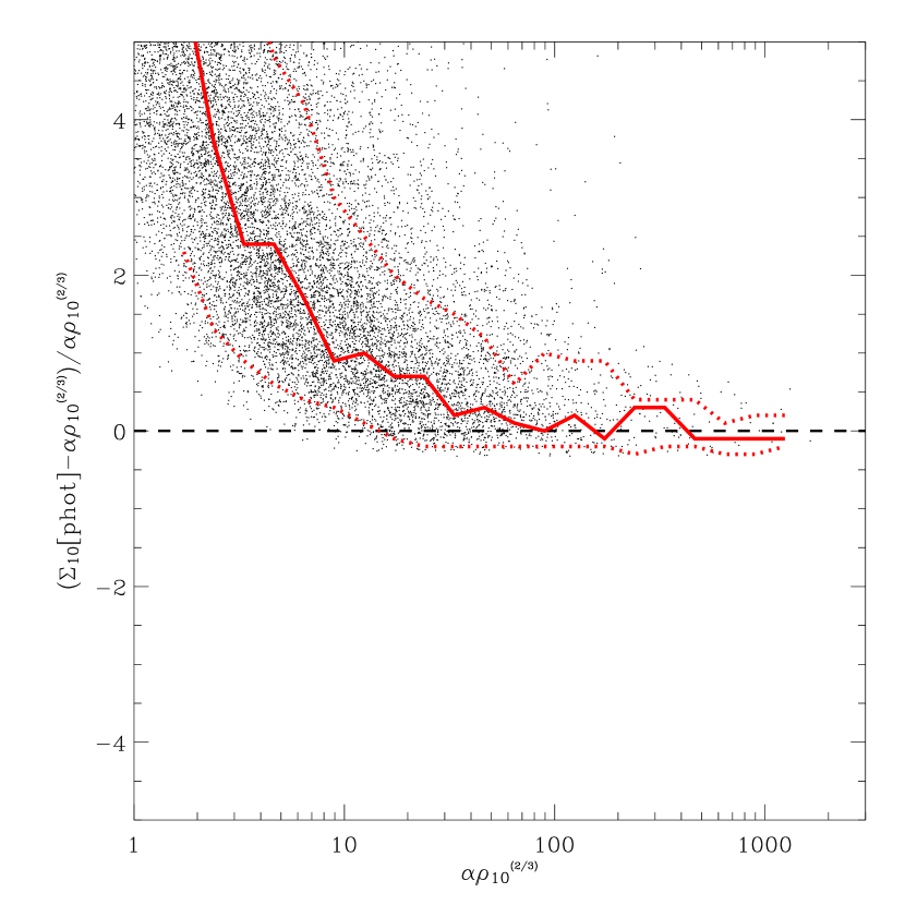
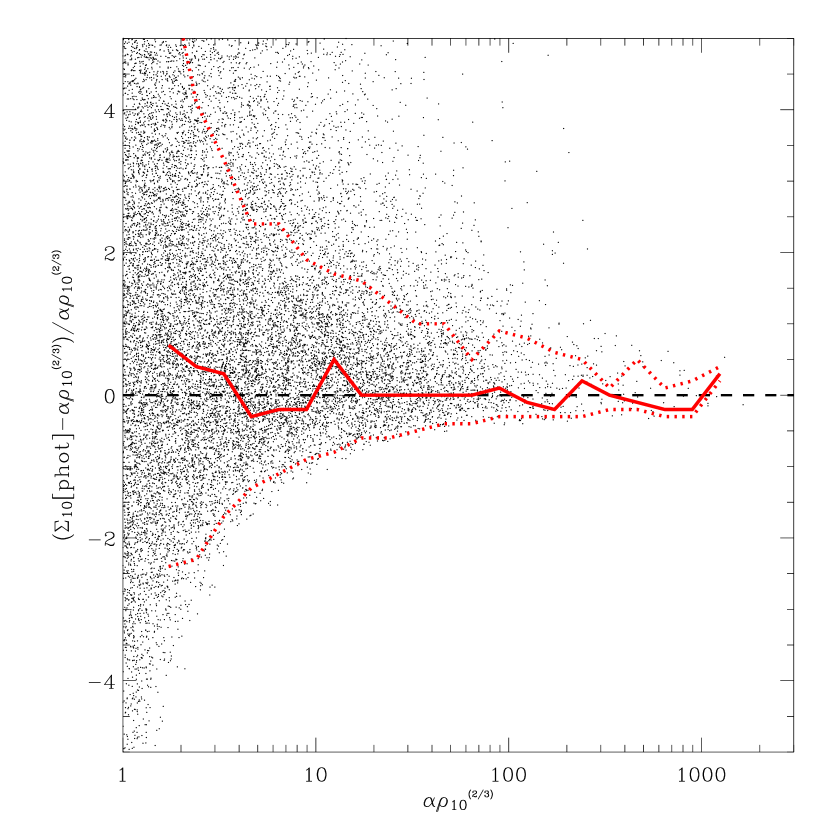
Figure 15.— Relative difference between projected densities $\Sigma_{10}$ estimated as discussed in § 3.1 from a “photometric-redshift” mock sample and the “true” densities one would measure with full knowledge of 3D galaxy positions in the same sample. The true density is converted into a projected density as indicated. The left panel shows the comparison without the background subtraction described in § 3.1, while the right panel shows the complete background-subtracted estimates, as done on the real data. The solid line gives the median values within bins of constant logarithmic size in true density, while the dotted lines enclose the 68.3% confidence interval around this value.

References

- (1) Andreon, S., 1998, ApJ, 501, 533
- (2) Bardelli, S., Zucca, E., Zamorani, G., et al., 1998, MNRAS, 296, 599
- (3) Barnes, J., 1992, ApJ, 393, 484
- (4) Benitez, N., 2000, ApJ, 536, 571
- (5) Benson, A. J., Frenk, C. S., Baugh, C.M., 2001, MNRAS, 327, 1041
- (6) Capak, P., et al., 2007, ApJS, submitted (this volume)
- (7) Capak, P., Abraham, R.G., Ellis, R.S.,et al., 2007, ApJS, submitted (this volume)
- (8) Cappelluti, N., Hasinger, G., Brusa, M., et al., 2007, ApJS, in press (this volume, also astro-ph/0701196)
- Cassata et al. (2005) Cassata, P., Cimatti, A., Franceschini, A., et al., 2005, MNRAS, 357, 903
- (10) Cassata, P. Guzzo, L., Franceschini, A., et al., 2007, ApJS, in press (this volume)
- (11) Clowe, D., et al. 2006, A&A, 451, 395
- (12) Conselice, C., 2003, ApJS, 147, 1
- (13) Cooper, M. C., Newman, J. A., Madgwick, D. S., et al. 2005, ApJ, 634, 833
- (14) Cortese, L., Gavazzi, G., Boselli, A., et al., 2006, A&A, 453, 847
- Dressler (1980) Dressler, A., 1980, ApJ, 236, 351
- Dressler et al. (1997) Dressler, A., 1997, ApJ, 490, 577
- (17) Ferrari, C., Benoist, C., Maurogordato, S., Cappi, A. & Slezak, E., 2005, A&A, 430, 19
- Finoguenov et al. (2001) Finoguenov, A., Reiprich, T. H., Böhringer, H. 2001, A&A, 368, 749
- (19) Finoguenov, A., Guzzo, L., Hasinger, G., et al., 2007, ApJ, in press (this volume, also astro-ph/0612360)
- (20) Gavazzi, G., Cortese, L., Boselli, A., et al., 2003, ApJ, 597, 210
- (21) Giovanelli, Haynes, M. P., & Chincarini, G. L., ApJ, 300, 77
- (22) Gunn, J.E., & Gott, J.R.I., 1972, ApJ, 176, 1
- (23) amana T., Takada M. & Yoshida N. 2004, MNRAS, 350, 893
- (24) Hasinger, G., Cappelluti, N., Brunner, H., et al., 2007, ApJ, in press (this volume, also astro-ph/0612311)
- (25) Heymans, C., et al., 2006,MNRAS, 368, 1323
- Kaifu et al. (2000) Kaifu, N., et al. 2000, PASJ, 52, 1
- (27) Kaiser N. & Squires G., 1993, ApJ, 404, 441
- (28) King L. & Schneider P., 2001, A&A, 369, 1
- (29) Kitzbichler, M.G. & White, S.D.M., 2006, MNRAS, submitted (astro-ph/0609636)
- Kotov & Vikhlinin (2005) Kotov, O., & Vikhlinin, A., 2005, ApJ, 633, 781
- (31) Kodama, T., Smail, I., Nakata, F., Okamura, S., Bower, R.G., 2001, ApJ, 562, L9
- Koekemoer et al., (2007) Koekemoer, A., et al., 2007, ApJS, submitted (this volume)
- (33) Larson, R.B., Tinsley, B.M, Caldwell, C.N., 1980, ApJ, 237, 692
- (34) Leauthaud A. et al. 2007, ApJS, submitted (this volume)
- (35) Lilly, S., Le Fevre, O., Renzini, A., et al. 2007, ApJS, in press (this volume, also astro-ph/0612291)
- (36) Massey R. et al. 2007b, MNRAS in press (astro-ph/0608643)
- (37) Massey R. et al. 2007, ApJS, submitted (this volume)
- Mobasher et al. (2007) Mobasher, B., Capak, P., et al., 2007, ApJS, in press (this volume, also astro-ph/0612344)
- (39) Moore, B., Katz, N., Lake, G., Dressler, A., Oemler, A., 1996, Nature, 379, 613
- (40) Navarro J.F., Frenk C.S. & White S.D.M., 1996, ApJ, 462 563
- (41) Navarro J.F., Frenk C.S. & White S.D.M., 1997, ApJ, 490 508
- (42) Postman, M., Franx, M., Cross, N. J. G., 2005, ApJ, 623, 721
- (43) Quilis, V., Moore, B., Bower, R., 2000, Science, 288, 1617
- (44) Rhodes J., Refregier A., Groth E., 2000, ApJ, 536, 79
- (45) Rhodes, J. et al., 2007, ApJS, submitted (this volume)
- (46) Sakai, S., Kennicutt, R.C., van der Hulst, J.M., & Moss, C., 2002, ApJ, 578, 842
- Schneider et al. (1998) Schneider, P., van Waerbeke, L., Jain, B., & Kruse, G. 1998, MNRAS, 296, 873
- (48) Scoville, N.Z., Aussel, H., Brusa, M., et al., 2007, ApJS, in press (this volume, also astro-ph/0612305)
- (49) Scoville, N.Z., Benson, A., Blain, A.W., et al., 2007, ApJS, in press (this volume, also astro-ph/0612306)
- (50) Scoville, N.Z., Aussel, H., Benson, A., et al., 2007, ApJS, in press (this volume, also astro-ph/0612384)
- (51) Smith, G.P., Treu, T., Ellis, R.S., Moran, S.M., Dressler, A., 2005, ApJ, 620, 78
- (52) Treu, T., Ellis, R.S., Kneib, J.-P., et al., 2003, ApJ, 591, 53
- Taniguchi, Y. et al. (2007) Taniguchi, Y., Scoville, N., Murayama, T., et al., 2007, ApJ, in press (this volume, also astro-ph/0612295)
- Vikhlinin et al. (2005) Vikhlinin, A., Kravtsov, A., Forman, W., Jones, C., Markevitch, M., Murray, S. S., & Van Speybroeck, L., 2006, ApJ, submitted, astro-ph/0507092
- (55) Zucca, E., Ilbert, O., Bardelli, S., et al. (VVDS Team), 2006, A&A, 455, 879