A minimal model of parallel electric field generation in a transversely inhomogeneous plasma

Abstract

We study the generation of parallel electric fields by virtue of propagation of ion cyclotron waves (with frequency 0.3 $\omega_{ci}$) in the plasma with a transverse density inhomogeneity. Using two-fluid, cold plasma linearised equations, we show for the first time that $E_{\parallel}$ generation can be understood by an analytic equation that couples $E_{\parallel}$ to the transverse electric field of the driving ion cyclotron wave. We prove that the minimal model required to reproduce previous kinetic results on $E_{\parallel}$ generation is the two-fluid, cold plasma approximation in the linear regime. In this simplified model, the generated $E_{\parallel}$ amplitude e.g. for plausible solar coronal parameters attains values of $\approx 90$ Vm^-1 for the mass ratio $m_{i}/m_{e}=262$, within a time corresponding to 3 periods of the driving ion cyclotron wave. By considering the numerical solutions we also show that the cause of $E_{\parallel}$ generation is electron and ion flow separation (which is not the same as electrostatic charge separation) induced by the transverse density inhomogeneity. The model also correctly reproduces the previous kinetic results in that only electrons are accelerated (along the background magnetic field), while ions do not accelerate substantially. We also investigate how $E_{\parallel}$ generation is affected by the mass ratio and found that amplitude attained by $E_{\parallel}$ decreases linearly as inverse of the mass ratio $m_{i}/m_{e}$, i.e. $E_{\parallel}\propto 1/m_{i}$. This result contradicts to the earlier suggestion by Génot et al (1999, 2004) that the cause of $E_{\parallel}$ generation is the polarisation drift of the driving wave, which scales as $\propto m_{i}$. Also, for realistic mass ratio of $m_{i}/m_{e}=1836$ our empirical scaling law is producing $E_{\parallel}=14$ Vm^-1 (for solar coronal parameters). Increase in mass ratio does not have any effect on final parallel (magnetic field aligned) speed attained by electrons. However, parallel ion velocity decreases linearly with inverse of the mass ratio $m_{i}/m_{e}$, i.e. parallel velocity ratio of electrons and ions scales directly as $m_{i}/m_{e}$. These results can be interpreted as following: (i) ion dynamics plays no role in the $E_{\parallel}$ generation; (ii) decrease in the generated parallel electric field amplitude with the increase of the mass ratio $m_{i}/m_{e}$ is caused by the fact that $\omega_{d}=0.3\omega_{ci}\propto 1/m_{i}$ is decreasing, and hence the electron fluid can effectively ”short-circuit” (recombine with) the slowly oscillating ions, hence producing smaller $E_{\parallel}$ which also scales exactly as $1/m_{i}$.

I Introduction and Motivation

The generation of parallel electric fields in inhomogeneous plasmas is a generic topic, which is of interest in a variety of plasma phenomena such as particle acceleration in Solar and stellar flares Fletcher (2005), auroral acceleration region and current sheets in the Earth magnetosphere (see refs. in Song and Lysak (2006)), laboratory plasma reconnection experiments Yamada et al. (1997); Matthaeus et al. (2005) and many more. In situ and remote observations of accelerated particles often show parallel electric fields in localised double layers, charge holes or U-shaped voltage drops.

In many astrophysical plasmas, an adequate form of description of large-scale, bulk dynamics is provided by Magnetohydrodynamics (MHD). However, MHD cannot provide proper description of some fundamental questions such as dissipation (which necessarily occurs at small-scales) and particle acceleration, unless the concept of somewhat uncertain from the fundamental point of view anomalous resistivity is invoked. The particle acceleration is of a considerable importance e.g. for Solar flares where the accelerated particles gain 50-80% of the energy released during this process. On one hand, observable dynamics e.g. (i) MHD waves in the case Solar plasmas; (ii) jets and accretion disks, in the case of stellar or compact objects or centres of Galaxies; and (iii) MHD waves in Tokamak spectroscopic studies; are well described by MHD theory. On the other hand, small-scale processes such as dissipation and particle acceleration are not observable directly. This creates controversy around issues such as the coronal heating problem (as to why the Solar corona is 200 times hotter than underlying photosphere); anomalous resistivity which manifests itself in an unusually fast damping of kink oscillations of solar coronal loops; or anomalous viscosity (problem of getting rid of angular momentum) in accretion disks. This dichotomy is schematically sketched in Fig. 1. Here energy cascade from the large scales to small scales is depicted as either $1/f=k^{-1}$ the white noise spectrum (in the case of waves) or some form of turbulence spectrum (with some power law of $k^{-\alpha}$ dependent on a particular turbulence model).

When MHD is used for the description of plasmas, the electric field is totally eliminated from the consideration. On one hand, this has a good justification due to the condition:

$$\frac{1}{c}\frac{\partial\vec{E}}{\partial t}/\left(\nabla\times\vec{B}\right)\approx\frac{1}{c}\frac{E}{T}\frac{L}{B}=\frac{1}{c}\frac{VB}{cT}\frac{L}{B}=\left(\frac{V}{c}\right)^{2}\ll 1,$$ (1)

i.e. for non-relativistic $(V\ll c)$ plasmas the ratio of the displacement and $(\nabla\times\vec{B})$ currents is much smaller than unity. Note that in the Eq.(1) spatial and time derivatives were approximated by: $\partial/\partial x\approx 1/L$ and $\partial/\partial t\approx 1/T$, where $L$ and $T$ are typical spatial and temporal scales of the system; and the ideal MHD limit ($\vec{E}=-\vec{V}\times\vec{B}/c$) was used. Thus, by neglecting the displacement current the electric field is totally excluded from the consideration. On one hand, this assumption may well be valid for the large scales. On the other hand, when the small scales are considered, the electric field, which appears (as we will show below) because of the electron and ion flow separation (which is impossible to treat correctly in single fluid MHD) starts to play far more important role than previously thought.

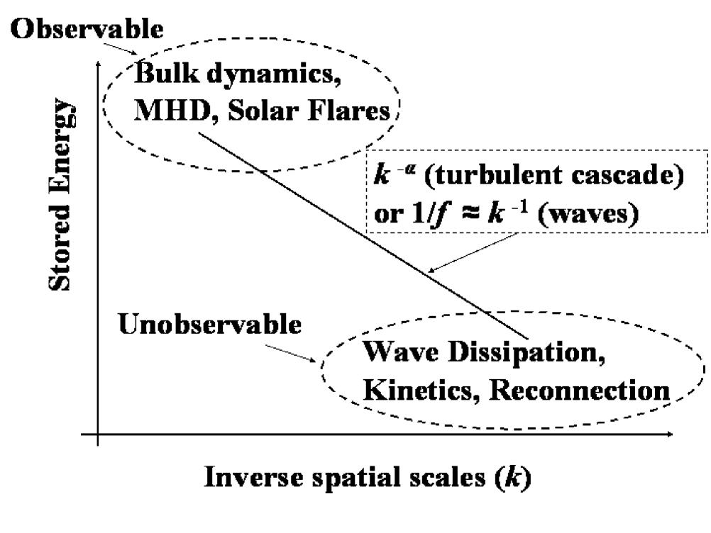
Figure 1: The sketch of typical power law spectrum of fluctuations along with their observability criteria.

Authors of Ref. Song and Lysak (2006) pointed out that previous studies of the $E_{\parallel}$ generation, based on the balance of the different terms in the generalised Ohm’s law, were not properly addressing the issue. In essence their main argument was that in such approach the generalised Ohm’s law merely states the Newton’s second law $F=ma$, whilst obscuring the true source of the parallel electric field generation. It was suggested that the source of $E_{\parallel}$ is the parallel displacement current. As stated above, this term is usually ignored, however in the regions of low density, for a certain $(\nabla\times\vec{B})_{\parallel}$, the plasma is too dilute to carry significant $J_{\parallel}$ and thus $(1/c)\partial E_{\parallel}/\partial t$ becomes important Song and Lysak (2006). One of the main conclusions that immediately follows is that the signatures of the generated $E_{\parallel}$ in space plasmas should be correlated with low plasma density.

Yet another series of works exist, which investigate the generation of parallel electric fields by virtue of propagation of Alfvén waves (or more precisely ion-cyclotron waves, see below) in the plasma with a transverse density inhomogeneity Génot et al. (1999, 2004); Tsiklauri et al. (2005a, b); Mottez et al. (2006); Tsiklauri (2006a, b). To this day the true cause of the generation of $E_{\parallel}$ in these studies eluded determination. Authors of Ref. Génot et al. (1999) considered the case of both transverse and longitudinal density inhomogeneity, applicable to the stratified Earth magnetosphere. They demonstrated that $E_{\parallel}$ is generated in the regions of transverse density gradients, and presented an analytical model in which the $E_{\parallel}$ and $E_{\perp}$ are coupled via longitudinal density gradient (see Eq.(6) from Ref. Génot et al. (1999)). Subsequently, detailed numerical study of long term evolution of the system was presented, including the generation of $E_{\parallel}$ Génot et al. (2004). However, in Ref.Génot et al. (2004) only the case of transverse density inhomogeneity was considered, while theoretical explanation was still based on Ref. Génot et al. (1999). This seems incorrect because the latter reference attributes $E_{\parallel}$ and $E_{\perp}$ coupling to the longitudinal inhomogeneity, which is absent in Ref. Génot et al. (2004). In brief, these two works suggest that the Alfvén wave propagation on sharp density gradients leads to the formation of a significant parallel electric field. It results from an electric charge separation generated on the density gradients by the polarisation drift associated with the time varying Alfvén wave electric field Génot et al. (2004). Their approach involved substituting ion polarisation drift current (electron one was omitted because of its proportionality to the particle mass) $j_{\perp}=(m_{i}n_{i}/B^{2})\partial E_{\perp}/\partial t$ into the Maxwell equations, which with the aid of the conservation laws yielded the equation for $E_{\parallel}$ and $E_{\perp}$ coupling Génot et al. (1999). Unaware of these works authors of Refs. Tsiklauri et al. (2005a, b) considered similar physical system with the increased density in the middle of the domain (mimicking) solar coronal loop, as opposed to Earth magnetospheric density cavity case studied in Refs. Génot et al. (1999, 2004). Similar effect of $E_{\parallel}$ generation was found because of the existence of density gradients in the system. Later a comment paper was published Mottez et al. (2006), which detailed similarities and differences of the two series of works.

It should be noted in passing that at that time we came to the realisation that electron acceleration seen in both series of works Génot et al. (1999, 2004); Tsiklauri et al. (2005a, b) is a non-resonant wave-particle interaction effect. In Refs. Tsiklauri et al. (2005a, b) the electron thermal speed was $v_{th,e}=0.1c$ while the Alfvén speed in the strongest density gradient regions was $v_{A}=0.16c$; this unfortunate coincidence led us to the conclusion that the electron acceleration by parallel electric fields was affected by the Landau resonance with the phase-mixed Alfvén wave. In Refs. Génot et al. (1999, 2004) the electron thermal speed was $v_{th,e}=0.1c$ while the Alfvén speed was $v_{A}=0.4c$ because they considered a more strongly magnetised plasma applicable to Earth magnetospheric conditions. Based on this observation, Refs. Tsiklauri (2006a, b) explored the possibility of $E_{\parallel}$ generation in the MHD description in the solar coronal heating problem context. Although, in the latter approach, the heating aspect seems certain (because the fast magnetosonic waves, which are generated by the interaction of weakly non-linear Alfvén wave with the transverse density inhomogeneity, dissipate on the bulk Braginkii resistivity), the issue whether such $E_{\parallel}$ can accelerate particles is less clear Tsiklauri (2006b).

II The model and results

The above discussion demonstrates that the issue of true cause of $E_{\parallel}$ generation when an Alfvén wave moves in the transversely inhomogeneous plasma eluded identification. In this work we present a minimal model which can explain $E_{\parallel}$ generation in mathematically and physically rigorous manner. We start from two-fluid, cold (ignoring thermal pressure) plasma linearised equations Krall and Trivelpiece (1973):

$$\partial_{t}\vec{V}_{e}=-(e/m_{e})\left(\vec{E}+\vec{V}_{e}\times\vec{B}_{0}/c\right),\\$$ (2)

$$\partial_{t}\vec{V}_{i}=+(e/m_{i})\left(\vec{E}+\vec{V}_{i}\times\vec{B}_{0}/c\right),$$ (3)

$$\partial_{t}\vec{B}=-c\nabla\times\vec{E},$$ (4)

$$\partial_{t}\vec{E}=c\nabla\times\vec{B}-4\pi ne(\vec{V}_{i}-\vec{V}_{e}).$$ (5)

Hereafter subscripts under $\partial$ denote partial derivative with respect to that subscript. Uniform, background magnetic field, $B_{0}$ is in $z$-direction. Density profile is specified as a ramp, $n(x)=n_{0}\left(1+3\exp\left[-[(x-100\delta)/(20\delta)]^{6}\right]\right)$ in which the central region (along $x$-direction, i.e. across $z$), is smoothly enhanced by a factor of 4, and there are the strongest density gradients having a width of about $20\delta$ around the points $x=81\delta$ and $x=119\delta$. Here $\delta=c/\omega_{pe}$ is the (electron) skin depth, which is a unit of grid in our numerical simulation. We use 2.5D description meaning that we keep all three, $x,y,z$ components of all vectors, however spatial derivatives $\partial/\partial y\equiv 0$. The above normalised plasma number density and Alfvén speed profiles are shown in Fig.(2).

In order to derive the equation that describes $E_{\parallel}=E_{z}$ generation, we write Eqs.(2)-(5) in $x,y,z$ component form. Omitting details of the calculation we present the final result:

$$\left(\partial^{2}_{tt}-c^{2}\partial_{xx}^{2}+\omega_{pi}^{2}+\omega_{pe}^{2}\right)E_{\parallel}=-c^{2}\partial^{2}_{zx}E_{x}.$$ (6)

Also, a similar calculation enables us to obtain the equation describing the dynamics of driving transverse electric field $E_{x}$ of an ion cyclotron wave:

$$\left(\partial^{2}_{tt}-c^{2}\partial_{zz}^{2}+\omega_{pi}^{2}+\omega_{pe}^{2}\right)E_{x}=$$

$$-c^{2}\partial^{2}_{zx}E_{\parallel}-\omega_{pi}^{2}(m_{i}/e)\omega_{ci}V_{iy}-\omega_{pe}^{2}(m_{e}/e)\omega_{ce}V_{ey}.$$ (7)

In the considered problem $E_{x}$ and $B_{y}$ are both components of Alfvén (ion cyclotron) wave, so these can be used interchangeably. Note that Eq.(7) also describes the feedback of the generated $E_{\parallel}$ on the driving transverse electric field $E_{x}$ (see the first term on the right-hand-side). Here the notation is standard: $\omega_{pe}=\sqrt{4\pi n_{0}e^{2}/m_{e}}$ and $\omega_{pi}=\sqrt{4\pi n_{0}e^{2}/m_{i}}$ are electron and ion plasma frequencies; $\omega_{c(e,i)}=eB_{0}/(m_{(e,i)}c)$ are respective cyclotron frequencies.

It is interesting to note that Eqs.(6) and (7) can be also obtained from the dielectric permeability tensor of cold, magnetised plasma (e.g. chapter 4.9 in Ref.Krall and Trivelpiece (1973)). For example, Eq.(6) can be directly obtained from the classical equation for the electric field perturbation, $\vec{E}_{1}$, in the case of $\vec{E}_{0}=0$ and $\vec{B}_{0}=B_{0}\hat{z}$

$$\nabla\times\nabla\times\vec{E}_{1}=(\omega^{2}/c^{2})\breve{\varepsilon}\vec{E}_{1},$$ (8)

where $\breve{\varepsilon}$ is the dielectric permeability tensor of cold, magnetised plasma. In effect, Eq.(6) can be obtained from the $z$-component of Eq.(8) and putting in $\varepsilon_{zz}=1-\omega_{pe}^{2}/\omega^{2}-\omega_{pi}^{2}/\omega^{2}$.

Figure 2: Dimensionless number density, open squares, and Alfvén speed, solid line, profiles across the uniform unperturbed magnetic field (i.e. along $x$-coordinate) which is used as an equilibrium configuration in our model of a footpoint of a solar coronal loop or a polar region plume.

In order to solve Eqs.(2)-(5) numerically we use the following normalisation: $t=\tilde{t}\omega_{pe}^{-1}$, $V_{x,y,z}=\tilde{V}_{x,y,z}c$, $E_{x,y,z}=\tilde{E}_{x,y,z}(m_{e}c\omega_{pe}/e)=\tilde{E}_{x,y,z}E_{0}$, $B_{x,y,z}=\tilde{B}_{x,y,z}B_{0}$, and $(x,y,z)=c/\omega_{pe}(\tilde{x},\tilde{y},\tilde{z})$. In what follows we omit tilde on the dimensionless quantities. The $(x,z)$ simulation 2D box size is $200\delta\times 2500\delta$. Since we fix background plasma number density at $10^{9}$ cm^-3 (typical value for the solar corona), $\omega_{pe}$ is then $1.784\times 10^{9}$ rad s^-1 and the simulation box size is $33.6$ m in $x$- and $420.5$ m in $z$-direction. $B_{0}$ was fixed at 101.5 Gauss (typical value for the solar corona), which gives $\omega_{ce}/\omega_{pe}=1$. $m_{i}/m_{e}$ ratio was varied as: 45.9, 91.8, 183.6, 262.286 (realistic one is 1836). These values correspond to $1/40,\;1/20,\;1/10$ and $1/7$-th of the realistic value respectively. This yields respectively: $\omega_{ci}/\omega_{pi}=B_{0}/(c\sqrt{4\pi n_{i}m_{i}})=V_{A}/c=1/\sqrt{m_{i}/m_{e}}=0.148,\;0.104,\;0.074$ and $0.062$ for $x\leq 70$ and $x\geq 130$ (realistic $\omega_{ci}/\omega_{pi}=V_{A}/c$ is 0.023). Here parameters are similar to e.g. Refs.Tsiklauri et al. (2005a, b), except for far more realistic mass ratios. Note that the simulation parameters are still somewhat artificial. Full kinetic, Particle-In-Cell (PIC) simulations employed in Refs.Tsiklauri et al. (2005a, b) or in gyro-kinetic approach which uses guiding centre approximation for electrons, whilst retaining ion particle-like dynamics Génot et al. (1999, 2004) are computationally challenging. Thus, in those studies rather modest mass ratios e.g. 16 were used. Note also, that since here we do not need to resolve electron thermal motions as we are only studying electromagnetic part of the problem ($E_{\parallel}$ generation) our unit of spatial grid size is $\delta=c/\omega_{pe}$, the (electron) skin depth. While in full kinetic, PIC simulation Tsiklauri et al. (2005a, b) the unit of grid has to be $\Delta=v_{th,e}/\omega_{pe}$. Since in a PIC simulation typically $v_{th,e}/c=0.1$, in the present, two-fluid approach an equivalent to PIC numerical simulation requires $(\delta/\Delta)^{2}=(c/v_{th,e})^{2}=10^{2}$ less grid points, thus it can be 100 times faster. For comparison a single run for mass ration 16 in Refs.Tsiklauri et al. (2005a, b) takes about 8 days on parallel, 32 dual-core 2.4 GHz Xeon processors, similar run with mass ratio of 262 would have taken 4 months. The numerical run presented here for the mass ratio of 262 takes 4 days with only one processor.

We solve relativistic version of Eqs.(2)-(5) numerically with a specially developed and tested FORTRAN 90 code which uses 4-th order centred spatial derivatives and 4-th order Runge-Kutta time marching. Although Alfvén speeds considered are at most $\approx 15$ % of the speed of light for $m_{i}/m_{e}=45.9$, relativistic effects were included. The simplest option becomes available in the linear regime. In ref. Krall and Trivelpiece (1973), appendix I, paragraph 5, it was shown that the relativistic equation of motion of a particle with charge $q$ and the rest mass $m_{0}$ can be written as

$$\frac{d}{dt}\vec{V}=\frac{q}{\gamma m_{0}}\left[\vec{E}+\frac{\vec{V}\times\vec{B}}{c}-\frac{\vec{V}(\vec{V}\cdot\vec{E})}{c^{2}}\right],$$ (9)

where $\gamma=(1-V^{2}/c^{2})^{-1/2}$. As can be seen from the latter equation, in the linear regime, it coincides with either Eq.(2) or (3) after substituting $m_{e,i}\to\gamma_{e,i}m_{e,i}$, where $\gamma_{e,i}=(1-V_{e,i}^{2}/c^{2})^{-1/2}$. Naturally, such simplified approach is only valid when there are no flows in the unperturbed state $V_{0}=0$. As can be seen below, largest attained velocities in the simulation are those of electrons, and these do not exceed 3 % of speed of light. Thus, relativistic corrections play only a minor role. It should be noted, however we still retain the displacement current in Eq.(5). Note, also that the gradients in the code are resolved numerically to an appropriate precision (20 grid points (open squares) across each gradient in Fig.(2)).

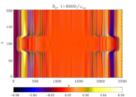
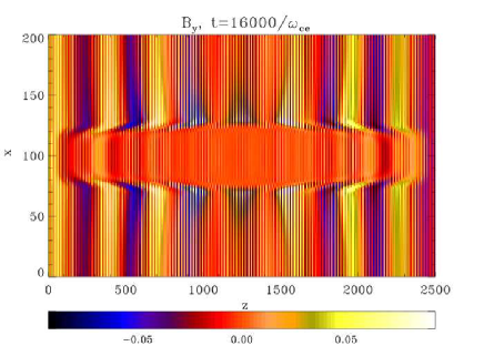
Figure 3: Contour (intensity) plots of phase-mixed transverse magnetic field $B_{y}$ at times $t=8000/\omega_{ce}$ (left) and $t=16000/\omega_{ce}$ (right).

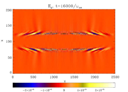
Figure 4: Contour (intensity) plots of $E_{z}=E_{\parallel}$ at times $t=8000/\omega_{ce}$ (left) and $t=16000/\omega_{ce}$ (right).

Initially all perturbations are set to zero, and we start driving the $z=1$ cell with the transverse magnetic fields of the form $B_{y}=-0.05\sin(\omega_{d}t)\left(1.0-\exp[-(t/(3.125\omega^{-1}_{ci}))^{2}]\right)$ and $B_{x}=-0.05\cos(\omega_{d}t)\left(1.0-\exp[-(t/(3.125\omega^{-1}_{ci}))^{2}]\right)$. As in Refs.Tsiklauri et al. (2005a, b), we fixed $\omega_{d}$ at 0.3 $\omega_{ci}$ (to avoid ion-cyclotron damping playing any role). $\left(1.0-\exp[-(t/(3.125\omega^{-1}_{ci}))^{2}]\right)$ factor ensures that these driving $B_{\perp}$ fields ramp up to their maximal values in time $t=3.125\omega_{ci}^{-1}$. Such driving with $B_{\perp}$ of 5% of the background $B_{0}$ excites circularly polarised ion-cyclotron (IC) waves, these waves are often misquoted as Alfvén waves Génot et al. (1999, 2004); Tsiklauri et al. (2005a, b). For parallel to $\vec{B}_{0}$ propagation, and assuming plasma quasi-neutrality, the relevant dispersion relation reads as Krall and Trivelpiece (1973):

$$k^{2}_{R,L}=\frac{\omega^{2}}{c^{2}}\left[1-\frac{\omega^{2}_{pe}+\omega^{2}_{pi}}{(\omega\mp\omega_{ce})(\omega\pm\omega_{ci})}\right],$$ (10)

where subscripts $R,L$ refer to the waves with right and left circular polarisation, and so are the upper and lower signs in the plus and minus. In the frequency range $\omega\ll\omega_{ci}$ both left and right polarised waves tend to an Alfvén wave branch, which satisfies the following dispersion relation Krall and Trivelpiece (1973):

$$k^{2}_{R,L}=\frac{\omega^{2}}{c^{2}}\left[1+\frac{4\pi n(m_{e}+m_{i})c^{2}}{B^{2}}\right],$$ (11)

which is the same as

$$\frac{\omega}{k}=V_{A}/\sqrt{1+V^{2}_{A}/c^{2}}.$$ (12)

Note, that the root in the denominator appears only because of the displacement current is kept. At frequencies $\omega\simeq 0.3\omega_{ci}$ however, the correct term ion-cyclotron wave instead of Alfvén wave should be used.

Note that in differ to Refs.Tsiklauri et al. (2005a, b) we now directly drive transverse magnetic fields ($B_{x},B_{y}$) (which in turn are coupled to transverse electric fields ($E_{x},E_{y}$)). Conventionally, Alfvénic and IC waves are more associated with magnetic field oscillation. However, in the kinetic, Particle-In-Cell simulation usually variation of electric field is used for driving waves, because particles respond to electric, rather than magnetic fields (both are naturally coupled, such as $E_{x}$ and $B_{y}$ represent single Alfvén wave). In the two-fluid numerical code like the one used here, it is possible to use transverse magnetic fields for driving of IC wave.

II.1 case of $m_{i}/m_{e}=262$

In this subsection we consider case of $m_{i}/m_{e}=262.268\approx 262$, which is the largest value considered in this study. As can be seen in Fig.(3), the generated at the left edge ($z=1$) IC waves propagate both in the directions of positive and negative $z$’s. However, because of the periodic boundary conditions used (applied on all physical quantities) IC wave that travels to the direction of negative $z$’s (to the left) re-appears on the right edge of the figure. As in all previous phase-mixing simulations Alfvén velocity is a function of the transverse (to the background magnetic field) coordinate, $x$, i.e. $V_{A}=V_{A}(x)\propto 1/\sqrt{n(x)}$ (see Fig.(2)). Thus as can be seen in Fig.(3) the IC wave middle portion travels slower than the parts close to the simulation box edge. This creates progressively strong transverse gradients and hence smaller spatial scales. If resistive effects are included (these are absent here), such configuration usually produces greatly enhanced dissipation and IC wave amplitude decays in space as $\propto\exp(-z^{3})$ Tsiklauri et al. (2005a, b). The $E_{\parallel}=E_{z}$ field dynamics is shown in Fig.(4).

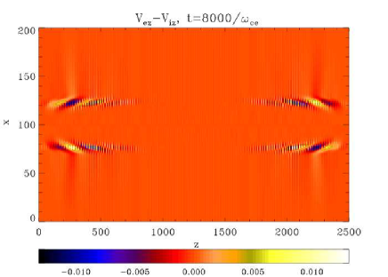
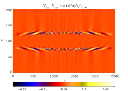
Figure 5: Contour (intensity) plots of $(V_{ez}-V_{iz})\propto j_{z}$ at times $t=8000/\omega_{ce}$ (left) and $t=16000/\omega_{ce}$ (right).

We gather that $E_{\parallel}$ is generated only in the regions of density gradients i.e. along $x=81$ and $x=119$ lines. This can be explained by analysing right-hand-side (RHS) of Eq.(6). $E_{\parallel}=0$ at $t=0$ everywhere, however it can only be generated in the regions where $\partial_{x}E_{x}\not=0$. The latter is true only in the density gradient regions where $E_{x}$ becomes progressively oblique propagating. Thus, Eq.(6), derived here for the first time, correctly explains the simulated process of $E_{\parallel}$ generation by IC waves. It should be also noted that this equation contains $\partial_{xx}^{2}$, which correctly accounts for the transverse (along $x$) propagation of the generated $E_{\parallel}$. $E_{\parallel}$’s longitudinal (along $z$) propagation due to the motion of IC wave along $z$-axis is indeed corroborated both by Fig.(3) and Eq.(7) - note $\partial_{zz}^{2}$ term. Also, note that $E_{\parallel}$ amplitude at time $t=16000\omega_{ce}^{-1}$ attains value of $3\times 10^{-5}$. This is somewhat smaller value than the one obtained in the full kinetic (PIC) simulation Tsiklauri et al. (2005a, b). This is due to the different mass ratios: in the the kinetic (PIC) simulation $m_{i}/m_{e}=16$, but here it is 262. In dimensional units this $E_{\parallel}$ corresponds to about 0.003 statvolt cm^-1 or 90 V m^-1, i.e. in such electric field electrons would be accelerated to the energy of $\approx 10$ keV over the distance of 100 m. Note, however, that the generated $E_{\parallel}$ is oscillatory in space and time.

In Fig.(5) we present $(V_{ez}-V_{iz})$ which is proportional to $j_{z}$, the parallel (electron and ion flow separation) current. It can be seen from this figure that $(V_{ez}-V_{iz})$ attains moderate values of $\approx 0.03c$. Authors of Ref.Génot et al. (2004) stated the importance of charge separation before. However the cause of $E_{\parallel}$ generation is actually electron and ion flow separation (see below). The latter is quite different from the electrostatic effect of charge separation, which is inherently a plasma kinetic effect. Electron and ion flow separation is a fluid-like (non-kinetic) effect, because their distribution functions remain Maxwellian at all times.

II.2 parametric study for different $m_{i}/m_{e}$’s

In this subsection we perform parametric study with different mass ratios $m_{i}/m_{e}$. This is particularly useful for understanding the physics of parallel electric field generation. This is needed because performing realistic mass ratio numerical simulation, $m_{i}/m_{e}=1836$, is computationally challenging.

Numerically challenging issues arise from the increase in mass ratio are the following:

(i) because our intention was to use a driving IC wave with $\omega_{d}=0.3\omega_{ci}$, when changing mass ratio, $w_{d}\propto 1/m_{i}$. Thus increasing mass of the ion leads to decrease in driving frequency. Since in all our numerical simulations we intended to have final simulation time of 3 driving IC wave periods, i.e. $t_{final}=3\times(2\pi/\omega_{d})\propto m_{i}$. Thus, in turn, increase in ion mass leads to increase in final simulation time. E.g. for the cases $m_{i}/m_{e}=$ 45.9, 91.8, 183.6, 262.286 considered here, the final simulation times were 2884, 5768, 11536 and 16000 $\omega^{-1}_{pe}$ respectively, i.e. $t_{final}\propto m_{i}$.

(ii) Increase in simulation time leads to the compulsory increase in the simulation domain size, $L$, in the direction along the magnetic field (direction of IC wave travel), i.e. $L=2\times(V_{A}/c)\times(3t_{final})\propto(1/\sqrt{m_{i}})\times m_{i}\propto\sqrt{m_{i}}$

Thus, as far as the slowdown of the numerical code is concerned, the combined slowdown effect of the above two factors is $m_{i}\sqrt{m_{i}}$.

In Fig.(6) we present time evolution of the amplitude of the generated parallel electric field, which we define as $\max(|E_{z}(x,z,t)|)$, i.e. at every time step we choose one point over whole simulation domain at which modulus of parallel electric field is the largest. This is, as it was shown above, along the strongest gradient lines $x=81\delta$ and $x=119\delta$. It can be seen from the graph that: (i) level attained by parallel electric field amplitude decreases with the increase in the mass ratio; (ii) rate at which the final amplitude is reached (the averaged slope, essentially) also decreases with the increase in the mass ratio.

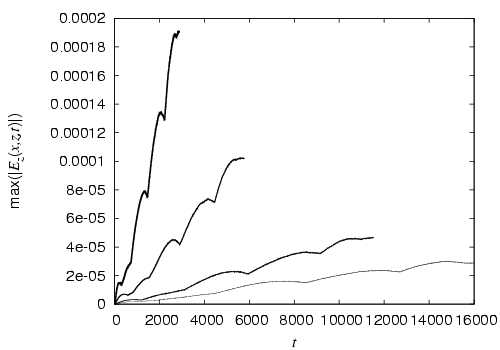
Figure 6: Time evolution of the amplitude of the generated parallel electric field, defined as $\max(|E_{z}(x,z,t)|)$. The thickest (upper left) line corresponds to $m_{i}/m_{e}=$ 45.9; while lines with decreasing thickness correspond to 91.8, 183.6, 262.286 respectively.

Exact behaviour of the final attained parallel electric field amplitude (within 3 periods of the driving ion cyclotron wave) as a function of mass ratio is shown in Fig. (7). Essentially this is a plot of the last data points (which are four) in the previous Fig. (6) as a function of $m_{i}/m_{e}$, i.e. $E^{*}=\max(|E_{z}(x,z,t_{final})|)$ vs. $m_{i}/m_{e}$. The dashed line corresponds to the fit $0.0085/(m_{i}/m_{e})$. Plotting such graph is very useful to establish the trend. Interestingly we see that that amplitude attained by $E_{\parallel}$ decreases linearly with inverse of the mass ratio $m_{i}/m_{e}$. The $x$-range in Fig.(7) is $m_{i}/m_{e}=30-1836$, so that rightmost point of the dashed line enables us to grasp $E_{\parallel}$ for the case of realistic mass ratio (i.e. 1836). We thus gather that $E_{\parallel}=0.0085/1836=4.630\times 10^{-6}$ which is $4.630\times 10^{-6}\times E_{0}=4.7\times 10^{-4}$ statvolt cm^-1 or 14 Vm^-1.

Figure 7: The final attained parallel electric field amplitude (generated within 3 periods of the driving ion cyclotron wave) as a function of mass ratio. Data points correspond to the last 4 data points in the previous Fig. (6). The dashed line corresponds to the fit $0.0085/(m_{i}/m_{e})$. This is a log-log plot.

In Figs. (8) and (9) we plot the amplitudes of the generated parallel flows of electron and ion fluids which we define as $\max(|V_{ez}(x,z,t)|)$ and $\max(|V_{iz}(x,z,t)|)$ respectively, i.e. at every time step we choose one point over whole simulation domain at which moduli of parallel flows of electrons and ions are the largest. Again, this occurs somewhere along the strongest gradient lines $x=81\delta$ and $x=119\delta$, because parallel electron and ion flows are confined to the strongest density gradient regions. Four different lies in each figure show the cases $m_{i}/m_{e}=$ 45.9, 91.8, 183.6, 262.286 considered. We gather from Figs. (8) and (9) that an increase in mass ratio does not have any effect on final parallel (magnetic field aligned) speed attained by electrons. However, parallel ion velocity decreases linearly with inverse of the mass ratio $m_{i}/m_{e}$. To investigate this more quantitatively, in Fig. (10) we plot the ratio of final attained electron and ion flow amplitudes (within 3 periods of the driving ion cyclotron wave) as a function of mass ratio. Essentially this is a plot of the ratio of last data points (which are four) in the Figs. (8) and (9) as a function of $m_{i}/m_{e}$, i.e. $V_{ratio}=\max(|V_{ez}(x,z,t_{final})|)/\max(|V_{iz}(x,z,t_{final})|)$ vs. $m_{i}/m_{e}$. The dashed line corresponds to the fit which is $(m_{i}/m_{e})$ with a slope of 1. i.e. parallel velocity ratio of electrons and ions scales directly as $m_{i}/m_{e}$.

Figure 8: Time evolution of the amplitudes of the generated parallel flows of electron fluid, defined as $\max(|V_{ez}(x,z,t)|)$. The thickest (upper left) line corresponds to $m_{i}/m_{e}=$ 45.9; while lines with decreasing thickness correspond to 91.8, 183.6, 262.286 respectively.

Figure 9: The same as in Fig. (8), but for ions.

III discussion

The conclusions that follow from the collective analysis of Figs.(6)–(10) initially may seem counterintuitive. On one hand maximal attained $E_{\parallel}$ amplitudes drop off as $1/m_{i}$ (Figs.(6)–(7)). On the other hand, electron flow maximal attained amplitudes do not depend on $m_{i}$ (they all are circa $0.03c$, see Fig.(8)), while ion flow maximal attained amplitudes drop off as $1/m_{i}$ (Figs. (9)–(10)). Thus one might expect that more massive ions should produce a bigger $E_{\parallel}$ (since separation of electron and ion fluids is the source of $E_{\parallel}$ and that separation is expected to be largest in the case of more massive ions, as they are slower). In fact, this is what would be expected if the polarisation drift produced by the driving IC wave is the cause of parallel electric field generation Génot et al. (1999, 2004). The latter two references use the following polarisation drift current:

$$j_{\perp}=\frac{m_{i}n_{i}}{B^{2}}\frac{\partial E_{\perp}}{\partial t},$$ (13)

where symbols have their usual meaning. The latter equation implies that $E_{\parallel}$ then should increase with $\propto m_{i}$. However, in Figs.(6)–(7) we see completely opposite $E_{\parallel}\propto 1/m_{i}$ scaling. These results can be interpreted (reconciled) as following: (i) ion dynamics plays no role in the $E_{\parallel}$ generation, i.e. polarisation drift has no effect in contrary to the claims of Refs. Génot et al. (1999, 2004); (ii) decrease in the generated parallel electric field amplitude with the increase of the mass ratio $m_{i}/m_{e}$ is caused by the fact that $\omega_{d}=0.3\omega_{ci}\propto 1/m_{i}$ is decreasing, and hence the electron fluid can effectively ”short-circuit” (recombine with) the slowly oscillating ions, hence producing smaller $E_{\parallel}$ which also scales exactly as $1/m_{i}$.

In summary, indeed, electron and ion fluid separation is causing $E_{\parallel}$ generation, but polarisation drift current produced by the driving IC wave plays no role.

Interestingly, by comparing Figs. (8) and (9) we gather that electron fluid is efficiently accelerated by the generated $E_{\parallel}$ to the velocities of up to $0.03c$, while ion fluid due to its larger inertia is much less mobile ($0.0001c-0.0007c$). This confirms yet another conclusion that was made in Refs.Tsiklauri et al. (2005a, b) which employed full kinetic simulation.

It should be noted that since here we use two-fluid approach the generated $E_{\parallel}$ cannot change the distribution function, which obviously remains Maxwellian, while in the previous kinetic simulation of a similar system it produced bumps in the distribution function as the electrons residing on the magnetic field lines with the density gradients get efficiently accelerated (see e.g. Fig.(4) in Ref.Tsiklauri et al. (2005b)).

Figure 10: The ratio of the final attained electron and ion flow amplitudes (within 3 periods of the driving ion cyclotron wave) as a function of mass ratio, i.e. $V_{ratio}=\max(|V_{ez}(x,z,t_{final})|)/\max(|V_{iz}(x,z,t_{final})|)$ vs. $m_{i}/m_{e}$. The dashed line corresponds to the fit which has a slope of 1 (note the direct correlation). This is a log-log plot.

IV Summary

We studied the generation of parallel electric fields by means of propagation of IC waves in the plasma with the transverse density inhomogeneity. By using simpler, than kinetic Génot et al. (1999, 2004); Tsiklauri et al. (2005a, b), two-fluid, cold plasma linearised equations, we show for the first time that $E_{\parallel}$ generation can be understood by an analytic equation that couples $E_{\parallel}$ to the transverse electric field. It should be noted that the generation of $E_{\parallel}$ is a generic feature of plasmas with the transverse density inhomogeneity and in a different context this was known for decades in the laboratory plasmas Cross and Miljak (1993); Ross et al. (1982). We prove that the minimal model required to reproduce the previous kinetic results of $E_{\parallel}$ generation is the two-fluid, cold plasma approximation in the linear regime. In the latter, the generated $E_{\parallel}$ amplitude attains values of $14$ Vm^-1 for plausible solar coronal parameters and realistic mass ratio of $m_{i}/m_{e}=1836$. By considering the numerical solutions for $(V_{ez}-V_{iz})$, we have shown that the cause of $E_{\parallel}$ appearance is the electron and ion flow separation (which is not the same as electrostatic charge separation) induced by the transverse density inhomogeneity.

We also investigate how $E_{\parallel}$ generation is affected by the mass ratio and found that amplitude attained by $E_{\parallel}$ (within 3 periods of the driving ion cyclotron wave) decreases linearly as $\propto 1/m_{i}$. This result contradicts to the earlier suggestion by Génot et al (1999, 2004) that the cause of $E_{\parallel}$ generation is the polarisation drift of the driving wave, which would suggest $E_{\parallel}\propto m_{i}$ scaling. Increase in mass ratio does not affect the final parallel (magnetic field aligned) speed attained by electron fluid. However, parallel ion velocity decreases linearly as $1/m_{i}$, this means that the parallel velocity ratio of electrons and ions scales directly as $m_{i}$.

It should be noted that when plasma density is homogeneous, no $E_{\parallel}$ generation takes place; and this is corroborated both by numerical simulations (not presented here) and agrees with the Eq.(6) (when $n=const$, the RHS of Eq.(6) is zero at all times as $E_{x}$ and $B_{y}$ do not propagate obliquely). Our model also correctly reproduces the previous kinetic results Génot et al. (1999, 2004); Tsiklauri et al. (2005a, b) that only electrons are accelerated (along the background magnetic field), while ions practically show no acceleration.

V appendix

Animations 1, 2, and 3 show movies corresponding to Figs.(3), (4) and (5) respectively. Note that horizontal axis indicates 500 grids, while the real simulation value is 2500. This is simply to reduce movie size, i.e. every 5-th point along the field was included in these movies.