Current sheet formation and non-ideal behaviour at three-dimensional magnetic null points

Abstract

The nature of the evolution of the magnetic field, and of current sheet formation, at three-dimensional (3D) magnetic null points is investigated. A kinematic example is presented which demonstrates that for certain evolutions of a 3D null (specifically those for which the ratios of the null point eigenvalues are time-dependent) there is no possible choice of boundary conditions which renders the evolution of the field at the null ideal. Resistive MHD simulations are described which demonstrate that such evolutions are generic. A 3D null is subjected to boundary driving by shearing motions, and it is shown that a current sheet localised at the null is formed. The qualitative and quantitative properties of the current sheet are discussed. Accompanying the sheet development is the growth of a localised parallel electric field, one of the signatures of magnetic reconnection. Finally, the relevance of the results to a recent theory of turbulent reconnection is discussed.

I Introduction

The three-dimensional topological structure of many astrophysical plasmas, such as the solar corona, is known to be highly complex. In order to diagnose likely sites of energy release and dynamic phenomena in such plasmas, where the magnetic Reynolds numbers are typically very large, it is crucial to understand at which locations strong current concentrations will form. These locations may be sites where singular currents are present under an ideal magnetohydrodynamic (MHD) evolution. In ideal MHD, the magnetic field is ‘frozen into’ the plasma, and plasma elements may move along field lines, but may not move across them. An equivalent statement of ideal evolution is that the magnetic flux through any material loop of plasma elements is conserved.

Three-dimensional (3D) null points and separators (magnetic field lines which join two such nulls) might be sites of preferential current growth, in both the solar corona Longcope (1996); Priest et al. (2005) and the Earth’s magnetosphere, see Refs. [Priest and Forbes, 2000; Siscoe, 1988] for reviews. 3D null points are thought to be present in abundance in the solar corona. A myriad of magnetic flux concentrations penetrate the solar surface, and it is predicted that for every 100 photospheric flux concentrations, there should be present between approximately 7 and 15 coronal null points Schrijver and Title (2002); Longcope et al. (2003); Close et al. (2005). Furthermore, there is observational evidence that reconnection involving a 3D null point may be at work in some solar flares (Fletcher et al., 2001) and solar eruptions Aulanier et al. (2000); Ugarte-Urra et al. (2007). Closer to home, there has been a recent in situ observation (Xiao et al., 2006) by the Cluster spacecraft of a 3D magnetic null, which is proposed to play an important role in the observed signatures of reconnection within the Earth’s magnetotail. In addition, current growth at 3D nulls has been observed in the laboratory Bogdanov et al. (1994).

While the relationship between reconnection at a separator (defined by a null-null line) and reconnection at a single 3D null point is not well understood, it is clear that the two should be linked in some way. Kinematic models anticipate that null points and separators are both locations where current singularities may form in ideal MHD Lau and Finn (1990); Priest and Titov (1996). Moreover, it is also expected that 3D nulls Bulanov and Olshanetsky (1984); Pontin and Craig (2005) and separators Longcope and Cowley (1996) may each collapse to singularity in response to external motions.

The linear field topology in the vicinity of a 3D magnetic null point may be examined by considering a Taylor expansion of ${\bf B}$ about the null;

$${\bf B}={\cal M}\cdot{\bf r},$$

where the matrix ${\cal M}$ is the Jacobian of ${\bf B}$ evaluated at the null Fukao et al. (1975); Parnell et al. (1996). The eigenvalues of ${\cal M}$ sum to zero since $\nabla\cdot{\bf B}=0$. The two eigenvectors corresponding to the eigenvalues with like-sign real parts define the fan (or $\Sigma$-) surface of the null, in which field lines approach (recede from) the null. The third eigenvector defines the orientation of the spine (or $\gamma$-) line, along which a single pair of field lines recede from (approach) the null [see Fig. 2(a)].

In Section II we discuss the nature of the evolution of the magnetic field in the vicinity of a 3D null, and provide an example which demonstrates that certain evolutions of the null are prohibited in ideal MHD. In Sections III and IV we present results of numerical simulations of a 3D null which is driven from the boundaries, and describe the qualitative and quantitative properties of the resulting current sheet. In Section V we observe that our models may point towards 3D nulls as a possible site where turbluent reconnection might take place. Finally in Section VI we give a summary.

II Non-ideal evolution around 3D nulls

II.1 Ideal and non-ideal evolution

The evolution of a magnetic field is said to be ideal if ${\bf B}$ can be viewed as being frozen into some ideal flow, i.e. there exists some ${\bf w}$ which satisfies

$${\bf E}+{\bf w}\times{\bf B}=-\nabla\Phi,$$ (1)

or equivalently

$$\frac{\partial{\bf B}}{\partial t}=\nabla\times\left({\bf w}\times{\bf B}\right)$$ (2)

everywhere. In order for the evolution to be ideal, ${\bf w}$ should be continuous and smooth, such that it is equivalent to a real plasma flow. Examining the component of Eq. (1) parallel to ${\bf B}$, it is clear that in configurations containing closed field lines, the constraint that $\oint{\bf E}\cdot{\bf dl}=0$ must be satisfied in order to satisfy Eq. (1), so that $\Phi$ is single-valued. However, even when no closed field lines are present, there are still configurations in which it may not be possible to find a smooth velocity ${\bf w}$ satisfying Eq. (1). These configurations may contain isolated null points, or pairs of null points connected by separators Lau and Finn (1990); Priest and Titov (1996); Longcope and Cowley (1996). We will concentrate in what follows on the case where isolated null points are present.

Even when non-ideal terms are present in Ohm’s law, it may still not be possible to find a smooth unique velocity ${\bf w}$ satisfying Eq. (2) if the non-ideal region is embedded in an ideal region (i.e. is spatially localised in all three dimensions), as this imposes a ‘boundary condition’ on $\Phi$ within the (non-ideal) domain. If field lines link different points (say ${\bf x}_{1}$ and ${\bf x}_{2}$) on the boundary between the ideal and non-ideal region, then this imposes a constraint on allowable solutions for $\Phi$ within the non-ideal region, since they must be consistent with $\Phi({\bf x}_{1})=\Phi({\bf x}_{2})$ Hornig and Priest (2003); Priest et al. (2003).

It has recently been claimed by Boozer Boozer (2002) that the evolution of the magnetic field in the vicinity of an isolated 3D null point can always be viewed as ideal. However, we will demonstrate in the following section that in fact certain evolutions of a 3D null are prohibited under ideal MHD, and must therefore be facilitated by non-ideal processes. Furthermore, in subsequent sections we will show that such evolutions are a natural consequence of typical perturbations of a 3D null.

The argument has been proposed (Boozer, 2002) that for generic 3D nulls

$$\nabla\times\left({\bf w}^{\prime}\times{\bf B}\right)\equiv{\bf w}^{\prime}\cdot\nabla{\bf B}=-\left(\frac{\partial{\bf B}}{\partial t}\right)_{{\bf x}_{0}}$$ (3)

at the null point, where ${\bf x}_{0}$ is the position of the null, which can always be solved for ${\bf w}^{\prime}$ so long as the matrix $\nabla{\bf B}$ is invertible. For a ‘generic’ 3D null with ${\rm det}(\nabla{\bf B})\neq 0$ this is always possible. However, Eq. (3) is only valid at the null itself, with solution ${\bf w}^{\prime}=d{\bf x}_{0}/dt$. In general, $\nabla\times\left({\bf w}^{\prime}\times{\bf B}\right)\neq{\bf w}^{\prime}\cdot\nabla{\bf B}$ in the vicinity of a given point. That is, it is not valid to discard the terms ${\bf B}(\nabla\cdot{\bf w}^{\prime})$ and $({\bf B}\cdot\nabla){\bf w}^{\prime}$ from the right-hand side of Eq. (2) (when expanded using the appropriate identity) when considering the behaviour of the flow around the null. In order to describe the evolution of the field around the null, we must consider the evolution in some finite (possibly infinitesimal) volume about the null. Under the assumption (3), the vicinity of the null moves like a ‘solid body’—which seems to preclude any field evolution. Thus, the equation simply states that the field null remains, supposing no bifurcations occur—it shows that the null point cannot disappear, but does not describe the flux velocity in any finite volume around the null. This argument—that the velocity of the null and the value of the flux-transporting velocity at the null need not necessarily be the same—has been made regarding 2D X-points by Greene Greene (1993).

Furthermore, in order to show that the velocity ${\bf w}^{\prime}$ is non-singular at the null, the assumption is made in Ref. [Boozer, 2002] that $\Phi$ can be uniquely defined at the null, and that it may be approximated by a Taylor expansion about the null, which clearly presumes that $\Phi$ is a well-behaved function. As will be shown in what follows, in certain situations, it is not possible to find a function $\Phi$ which is (or in particular whose gradient $\nabla\Phi$ is) well-behaved at the null point (smooth and continuous). This is demonstrated below by analysing the properties of the function $\Phi$ with respect to any arbitrary boundary conditions away from the null point itself. By beginning at the null point and extrapolating $\Phi$ outwards, it may indeed be possible to choose $\Phi$ to be well-behaved at the null, but this $\Phi$ must not be consistent with any physical (i.e. smooth) boundary conditions on physical quantities such as the plasma flow.

In fact, it has been proven by Hornig and Schindler Hornig and Schindler (1996) that no smooth ‘flux velocity’ or velocity of ‘ideal evolution’ exists satisfying Eq. (2) if the ratios of the null point eigenvalues change in time. They have shown that under an ideal evolution, the eigenvectors (${\bf q}_{\alpha}$) and eigenvalues ($\alpha$) of the null evolve according to

$$\frac{d{\bf q}_{\alpha}}{dt}={\bf q}_{\alpha}\cdot\nabla{\bf w},\qquad\frac{d\alpha}{dt}=C\alpha,$$ (4)

where $C=-\nabla\cdot{\bf w}|_{{\bf x}_{0}}$ is a constant. From the second equation it is straightforward to show that the ratio of any two of the eigenvalues must be constant in time.

Note finally that the assumption that ${\rm det}(\nabla{\bf B})\neq 0$ rules out the possibility of bifurcation of null points. While it is non-generic for ${\rm det}(\nabla{\bf B})=0$ to persist for a finite period of time, when multiple null points are created or annihilated in a bifurcation process, a higher order null point is present right at the point of bifurcation, and ${\rm det}(\nabla{\bf B})$ passes through zero. Such bifurcation processes are naturally occurring, and clearly require a reconnection-like process to take place.

II.2 Example

We can gain significant insight by considering the kinematic problem. We consider an ideal situation, so that Ohm’s law takes the form of Eq. (1). Uncurling Faraday’s law gives ${\bf E}=-\nabla\Phi^{\prime}-\frac{\partial{\bf A}}{\partial t}$, where ${\bf B}=\nabla\times{\bf A}$, and combining the two equations we have that

$$\nabla\widetilde{\Phi}+{\bf w}\times{\bf B}=\frac{\partial{\bf A}}{\partial t},$$ (5)

where $\widetilde{\Phi}=\Phi-\Phi^{\prime}$. We proceed as follows. We consider a given time-dependent magnetic field, and calculate the corresponding functions $\widetilde{\Phi}$ and ${\bf w}_{\perp}$. The component of ${\bf w}$ parallel to ${\bf B}$ is arbitrary with respect to the evolution of the magnetic flux. We choose the magnetic field such that we have an analytical parameterisation of the field lines, obtained by solving $\frac{d{\bf X}}{ds}={\bf B}({\bf X}(s))$, where the parameter $s$ runs along the field lines. Then taking the component of Eq. (5) parallel to ${\bf B}$ we have

$$\begin{array}[]{rcl}\nabla\widetilde{\Phi}\cdot{\bf B}&=&\frac{\partial{\bf A}}{\partial t}\cdot{\bf B}\\ \widetilde{\Phi}&=&\int\frac{\partial{\bf A}}{\partial t}\cdot{\bf B}\>ds,\end{array}$$ (6)

where the spatial distance $dl=|{\bf B}|ds$. Expressing ${\bf B}$ and $\frac{\partial{\bf A}}{\partial t}$ as functions of $({\bf X}_{0},s)$ allows us to perform the integration. This defines $\nabla_{\parallel}\widetilde{\Phi}$, while the constant of this integration, $\widetilde{\Phi}_{0}({\bf X}_{0})$, allows for different $\nabla_{\perp}\widetilde{\Phi}$. We now substitute in the inverse of the field line equations ${\bf X}_{0}({\bf X})$ to find $\widetilde{\Phi}({\bf X})$. Finally,

$${\bf w}_{\perp}=-\frac{(\frac{\partial{\bf A}}{\partial t}-\nabla\widetilde{\Phi})\times{\bf B}}{B^{2}}.$$ (7)

Consider now a null point, the ratios of whose eigenvalues change in time. Take the magnetic field to be

$${\bf B}=\left(-2x-yf(t),y+xf(t),z\right).$$ (8)

A suitable choice for $\frac{\partial{\bf A}}{\partial t}$ is $\frac{\partial{\bf A}}{\partial t}=-f^{\prime}/2\>(0,0,x^{2}+y^{2})$ (other appropriate choices lead to the same conclusions as below). The eigenvalues of the null point are

$$\lambda_{1}=1\qquad,\qquad\lambda_{\pm}=\frac{-1\pm\sqrt{9-4f^{2}}}{2},$$ (9)

with corresponding eigenvectors

$${\bf q}_{1} = (0,0,1)$$

$${\bf q}_{+} = \left(\frac{\lambda_{+}-1}{f},1,0\right)$$

$${\bf q}_{-} = \left(1,\frac{f}{\lambda_{-}-1},0\right).$$

From the above it is clear that the spine (defined by $(1,0,0)$ when $f=0$) is given by

$$z=0\quad,\quad(1-\lambda_{-})y+fx=0.$$

In addition, the equation of the fan plane (which lies at $x=0$ when $f=0$) can be found by solving ${\hat{\bf n}}\cdot{\bf r}=0$, $\hat{{\bf n}}={\bf q}_{1}\times{\bf q}_{+}$ to give

$$\frac{(1-\lambda_{+})}{f}\>y+x=0.$$

Thus the spine and fan of the null close up on one another in time (being perpendicular when $f(t)=0$), see Fig. 1(b). Note that we require $|f|<3/2$ to preserve the nature of the null point, otherwise is collapses to a non-generic null; we may take for example $f={\rm tanh}(t)$. In order to simplify what follows, we define two new functions $M$ and $P$ which describe the locations of the spine and fan of the null:

$$M(x,y,t) = \frac{(1-\lambda_{-})y+fx}{fx_{1}},$$ (10)

$$P(x,y,t) = \frac{(1-\lambda_{+})y+fx}{fx_{1}}.$$ (11)

II.2.1 Analytical field line equations

Now, the first step in solving the equations is to find a representation of the field lines. Solving $\frac{d{\bf X}}{ds}={\bf B}({\bf X}(s))$ gives

$$x = (\lambda_{+}-1)C_{1}e^{\lambda_{+}s}+(\lambda_{-}-1)C_{2}e^{\lambda_{-}s}.$$

$$y = fC_{1}e^{\lambda_{+}s}+fC_{2}e^{\lambda_{-}s}$$ (12)

$$z = z_{0}e^{s}$$

where $C_{1}$ and $C_{2}$ are constants. Clearly the equation for $z$ is simple, but the other two are coupled in a more complicated way. In order to render the field line equations invertible, we choose to set $s=0$ on surfaces which move in time, tilting as the null point does. This is allowable since there is no linking between the integration of the field lines and the time derivative, that is, $t$ (or $f$) is just a constant in the integration. We choose to set $s=0$ on surfaces defined by

$$x=x_{1}-\frac{1-\lambda_{+}}{f}y\quad,\quad y=y_{0}-\frac{x_{1}f}{\lambda_{+}-\lambda_{-}}$$ (13)

where $x_{1}$ is a constant and $y_{0}=y_{0}(x,y,t)$ is the starting position of the field line footpoint on the tilting surface. Then

$$C_{1}=\frac{y_{0}}{f}\quad,\quad C_{2}=\frac{-x_{1}}{\lambda_{+}-\lambda_{-}}.$$ (14)

We can see by comparison of equations (13) and (14) that our ‘boundaries’ lie parallel to the fan plane, but with a shift of $\pm x_{1}$.

With $C_{1}$ and $C_{2}$ now defined by Eq. (14), Eqs. (12) may be inverted to give

$$y_{0} = \frac{fx_{1}}{\lambda_{+}-\lambda_{-}}MP^{\lambda_{+}/\lambda_{-}},$$

$$z_{0} = zP^{-1/\lambda_{-}},$$ (15)

$$s = \frac{1}{\lambda_{-}}{\rm ln}P.$$

II.2.2 Solving for $\widetilde{\Phi}$ and physical quantities

The first step in determining the solution is to solve for $\widetilde{\Phi}$, which is given by

$$\widetilde{\Phi}=\int_{0}^{s}z(x^{2}+y^{2})\>ds$$ (16)

where $x$, $y$, $z$ are functions of $(y_{0},z_{0},s)$. Upon substitution of (12), it is straightforward to carry out the integration in a symbolic computation package (such as Maple or Mathematica), since the integrand is simply a combination of exponentials in $s$. We then substitute (II.2.1) into the result to obtain $\widetilde{\Phi}(x,y,z)$.

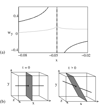
Figure 1: (a) Plots of $w_{y}$ against $x$ for $\widetilde{\Phi}_{0}=0$ (black line) and for the case where $\widetilde{\Phi}_{0}$ is defined by Eq. (17) (grey line). The dashed line indicates the location of the fan plane, and we take $f=0.2,x_{1}=1,y=0.7,z=0.5$. (b) Orientation of the null spine and fan for $t=0$ (left) and $t>0$ (right).

For any general choice of the function $\widetilde{\Phi}_{0}$ (i.e. choice of initial conditions for the integration, which may be viewed as playing the role of boundary conditions), we find that $\widetilde{\Phi}$ is non-smooth at the fan plane, and therefore $\nabla\widetilde{\Phi}$ tends to infinity there. Thus the electric field ${\bf E}$ and flux velocity ${\bf w}$ will tend to infinity at the fan plane (see Fig. 1(a)). Examining the expression for $\widetilde{\Phi}$, it is apparent that the problematic terms are those in $P^{-1/\lambda_{-}}$ (since $-1/\lambda_{-}<-1/2$ for $-1\leq f\leq 1$). In order to cancel out all of these terms, we must take (by inspection)

$$\widetilde{\Phi}_{0}=-x_{1}^{2}\>\frac{f^{2}+(1-\lambda_{-})^{2}}{(\lambda_{+}-\lambda_{-})^{2}(1+2\lambda_{-})}\>z_{0}.$$ (17)

With this choice, $\widetilde{\Phi}$ is smooth and continuous everywhere. However, $\nabla\widetilde{\Phi}$ is still non-smooth in the fan plane. Again examining $\widetilde{\Phi}$, we see that this results from terms in $P^{\mu_{1}}{\rm ln}P$ ($\mu_{1}$ constant). These take the form (after simplification)

$$\widetilde{\Phi} = ......-4fx_{1}y_{0}z_{0}s$$ (18)

$$= ......-\frac{4f^{2}x_{1}^{2}}{\lambda_{+}-\lambda_{-}}\>zP^{-1/\lambda_{-}}\>MP^{-\lambda_{+}/\lambda_{-}}\>{\rm ln}P^{-1/\lambda_{-}}.$$

Now, due to the form of $y_{0}(x,y,z,t)$ and $z_{0}(x,y,z,t)$ (Eq. II.2.1), it is impossible to remove the term in $P^{\mu_{1}}{\rm ln}P$ through addition of any $\widetilde{\Phi}_{0}(y_{0},z_{0})$ without inserting some term in either $z^{\mu_{2}}{\rm ln}z$ or $M^{\mu_{3}}{\rm ln}M$ ($\mu_{i}$ constant). This is simply equivalent to transferring the non-smoothness to the vicinity of the spine instead of the fan. Thus, there is no choice of boundary conditions which can possibly render the evolution ‘ideal’.

The example discussed above demonstrates that in an ideal plasma, it is not possible for a 3D null point to evolve in the way described, with the spine and fan opening/closing towards one another. Therefore, if such an evolution is to occur, non-ideal processes must become important.

III Resistive MHD simulations

We now perform numerical simulations in the 3D resistive MHD model. The setup of the simulations is very similar to that described by Pontin and Galsgaard Pontin and Galsgaard (2007). More details of the numerical scheme may be found in Refs. [Galsgaard and Nordlund, 1997; Archontis et al., 2004]. We consider an isolated 3D null point within our computational volume, which is driven from the boundary. We focus on the case where the null point is driven from its spine footpoints. The driving takes the form of a shear. We begin initially with a potential null point; ${\bf B}=B_{0}(-2x,y,z)$, and with the density $\rho=1$, and the internal energy $e=5\beta/2$ within the domain, so that we initially have an equilibrium. Here $\beta$ is a constant which determines the plasma-$\beta$, which is infinite at the null itself, but decreases away from it. We assume an ideal gas, with $\gamma=5/3$, and take $B_{0}=1$ and $\beta=0.05$ in each of the simulations. A stretched numerical grid is used to give higher resolution near the null (origin). Time units in the simulations are equivalent to the Alfvén travel time across a unit length in a plasma of density $\rho=1$ and uniform magnetic field of modulus 1. The resistivity is taken to be uniform, with its value being based upon the dimensions of the domain. Note that at $t=0$, ${\bf B}$ is scale-free as it is linear, and thus, the actual value of $\eta$ is somewhat arbitrary until we fix a physical length scale to associate with the size of our domain.

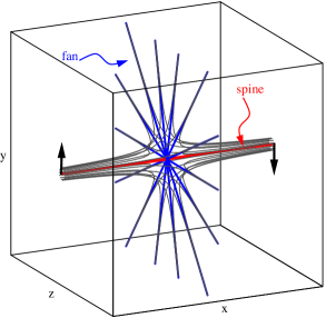
(a) (b)

Figure 2: (a) (Colour online) Schematic of the 3D null point in the computational domain. The black arrows indicate the direction of the boundary driving. (b) Boundary driving flow at $x=-X_{L}$, the lower $x$-boundary, for $Y_{l}=Z_{l}=3$ and $A_{d}=80$.

At $t=0$, the spine of the null point is coincident with the $x$-axis, and the fan plane with the $x=0$ plane [see Fig. 2(a)]. A driving velocity is then imposed on the (line-tied) $x$-boundaries, which advects the spine footpoints in opposite directions on the opposite boundaries (chosen to be in the $y$-direction without loss of generality). We choose an incompressible (divergence-free) velocity field, defined by the stream function

$$\psi=V_{0}(t)\cos^{2}\left(\frac{\pi y_{1}}{2}\right)\sin\left(\pi z_{1}\right)e^{-A_{d}(y_{1}^{2}+z_{1}^{2})},$$ (19)

where $y_{1}=y/Y_{l}$ and $z_{1}=z/Z_{l}$, the numerical domain has dimensions $[\pm X_{l},\pm Y_{l},\pm Z_{l}]$, and $A_{d}$ describes the localisation of the driving patch. This drives the spine footpoints in the $\pm{\hat{\bf y}}$ direction, but has return flows at larger radius (see Fig. 2(b)). Note however that the field lines in the return flow regions never pass close to the fan (only field lines very close to the spine do). We have checked that there are no major differences for the evolution from the case of uni-directional driving (${\bf v}=v_{y}{\hat{\bf y}}$).

Two types of temporal variation for the driving are considered. In the first, the spine is driven until the resulting disturbance reaches the null, forming a current sheet (see below), then the driving switches off. It is smoothly ramped up and down to reduce sharp wavefront generation. In the other case, the driving is ramped up to a constant value and then held there (for as long as numerical artefacts allow). Specifically, we take either

$$V_{0}(t)=v_{0}\left(\left(\frac{t-\tau}{\tau}\right)^{4}-1\right)^{2}\qquad,\qquad 0\leq t\leq\tau,$$ (20)

or

$$V_{0}(t)=v_{0}\tanh^{2}(t/\tau),$$ (21)

where $v_{0}$ and $\tau$ are constant. We begin by discussing the results of runs with the transient driving profile, as described by Eqs. (19) and (20).

III.1 Current evolution and plasma flow

Unless otherwise stated, the following sections describe results of a simulation run with the transient driving time-dependence, and with parameters $X_{l}=0.5$, $Y_{l}=Z_{l}=3$, $A_{d}=80$, $v_{0}=0.01$, $\tau=1.8$ and $\eta=10^{-4}$. The resolution is $128^{3}$, and the grid spacing at the null is $\delta x\sim 0.005$ and $\delta y,\delta z\sim 0.025$ (the results have been checked at $256^{3}$ resolution).

As the boundary driving begins, current naturally develops near the driving regions. This disturbance propagates inwards towards the null at the local value of the Alfvén speed. It concentrates at the null point itself, with the maximum of $J=|{\bf J}|$ growing sharply once the disturbance has reached the null, where the Alfvén velocity vanishes. Figure 3 shows isosurfaces of $J$ (at 50$\%$ of maximum).

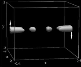
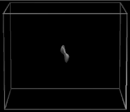
(a) (b) (c) (d)

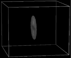
Figure 3: Isosurfaces of $J$, at 50$\%$ of the maximum at that time, for times marked by diamonds in Fig. 4 ($t=1,2,3,5$)

It is fruitful to examine the current evolution in a plane of constant $z$ (plane of the shear). In such a plane, the current forms an ‘S’-shape, and is suggestive of a collapse from an X-type configuration (spine and fan orthogonal) to a Y-type configuration in the shear plane (Fig. 5). Note that once the driving switches off, the current begins to weaken again and spreads out in the fan plane, and the spine and fan relax back towards their initial perpendicular configuration (see Figs. 3(d), 5(d)).

That we find a current concentration forming which is aligned not to the (global directions of the) fan or spine of the null (in contrast with simplified analytical self-similar Bulanov and Olshanetsky (1984) and incompressible Craig and Fabling (1996) solutions), but at some intermediate orientation, is entirely consistent with the laboratory observations of Bogdanov et al. Bogdanov et al. (1994). In fact the angle that our sheet makes in the $z=0$ plane (with, say, the $y$-axis) is dependent on the strength of the driving (strength of the current), as well as the field structure of the ‘background’ null (as found in Ref. [Bogdanov et al., 1994]) and the plasma parameters. We should point out that we consider the case where in the notation of Bogdanov et al. $\gamma<1$. They consider a magnetic field ${\bf B}=\left((h+h_{r})x,-(h-h_{r})y,-2h_{r}z\right)$, and define $\gamma=h_{r}/h$. Thus, for $\gamma>1$ they have current parallel to the spine, which we expect to be resultant from rotational motions, and have very different current sheet and flow structures Pontin and Galsgaard (2007); Pontin et al. (2004).

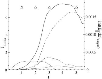
Figure 4: Evolution of the maximum value of each component of ${\bf J}$ ($J_{x}$ dotted, $J_{y}$ dot-dashed, $J_{z}$ solid), as well as the integral of $E_{\|}$ along the $z$-axis (dashed), and the time-variation of the boundary driving (triple-dot-dashed). The diamonds ($\bigtriangleup$) mark the times at which the isosurfaces of $J$ in Fig. 3 are plotted.

Now examine the temporal evolution of the maximum value of each component of the current (see Fig. 4). It is clear that the current component that is enhanced significantly during the evolution is $J_{z}$. This is the component which is parallel to the fan plane, and perpendicular to the plane of the shear (consistent with Ref. [Pontin and Galsgaard, 2007], and also with a collapse of the null’s spine and fan towards each other (see, e.g. Ref. [Parnell et al., 1996])).

Examining the plasma flow in the plane perpendicular to the shear, ($z$ constant) we find that it develops a stagnation-point structure, which acts to close up the spine and fan (see Fig. 5). It is worth noting that the Lorentz force acts to accelerate the plasma in this way, while the plasma pressure force acts against the acceleration of this flow (opposing the collapse). In the early stages after the current sheet has formed, the stagnation flow is still clearly in evidence, with plasma entering the current concentration along its ‘long sides’ and exiting at the short sides—looking very much like the standard 2D reconnection picture in this plane [Fig. 5(b)]. As time goes on, the driving flow in the $y$-direction begins to dominate.

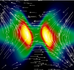
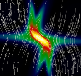
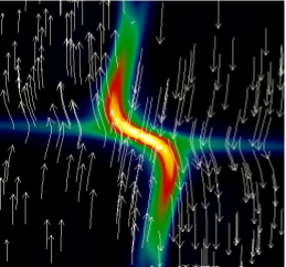
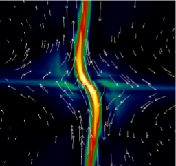
Figure 5: (Colour online) Arrows show plasma flow, while shading shows $|J|$ (scaled to the maximum in each individual frame). Viewed in the $z=0$ plane, inner 1/4 of domain: $[x,y]=[-0.12..0.12,-0.7..0.7]$ (y vertical). Images are at $t=1.6,2.4,3.0,5.0$.

III.2 Magnetic structure

As the evolution proceeds and the current becomes strongly concentrated at the null, this is naturally where the magnetic field becomes stressed and distorted. Firstly, plotting representative field lines which thread the sheet and pass very close to the null, we see that in fact the topological nature of the null is preserved [Fig. 6(a)]. That is, underlying the Y-type structure of the current sheet there is still only a single null point present, with the angle between the spine and the fan drastically reduced (see below).

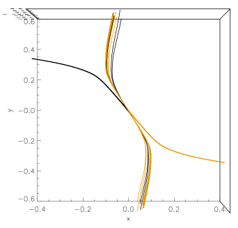
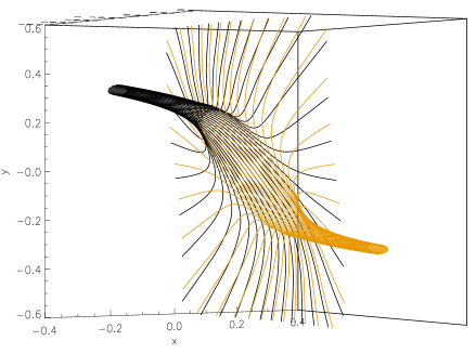
(a) (b)
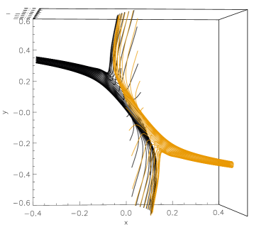
(c) (d)

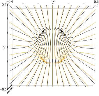
Figure 6: (Colour online) (a) Field lines traced from very close to the spine (black for negative $x$, grey (orange online) for positive). (b-d) The same, but for field lines traced from rings of larger radius around the spine and which graze the surface of the current sheet, viewed at different angles of rotation about the $y$-axis; (b) $\pi/36$, (c) $\pi/6$, (d) $\pi/2$. This simulation run uses continuous driving, with parameters $X_{l}=0.5$, $Y_{l}=Z_{l}=6$, $A_{d}=160$, $v_{0}=0.04$, $\tau=0.5$ and $\eta=5\times 10^{-4}$. Time of the images is $t=6$.

It is interesting to consider the 3D structure of the current sheet, that is the nature of the quasi-discontinuity of the magnetic field at the current sheet. This is important since the common conception of a ‘current sheet’ is a 2D Green-Syrovatskii sheet with anti-parallel field on either side of a cut in the plane (see Refs. [Green, 1965; Syrovatskii, 1971]). Here, however, a current sheet localised in all three dimensions is present.

In order to determine the structure of this 3D current sheet, we would like to know the nature of the jump ($\Delta{\bf B}$) in the magnetic field vector ${\bf B}$ across it, and how this varies throughout the sheet. Of course, because $\eta\neq 0$, there is no true discontinuity in ${\bf B}$, though the jump $\Delta{\bf B}$ would occur over a shorter and shorter distance if $\eta$ were decreased (in an external domain of fixed size). This mismatching in ${\bf B}$ may be visualised by plotting field lines which define approximately the boundaries of the current sheet, see Fig. 6(b-d). Along $z=0$ between the two ends of the current sheet, the black and grey (orange online) field lines (on opposite sides of the current concentration) are exactly anti-parallel [see Fig. 6(d)]. Thus in this plane (only) we have something similar to the 2D picture (due to symmetry). However, for $z\neq 0$, the magnetic field vectors on either side of the current sheet are not exactly anti-parallel, and the black and grey (orange online) field lines cross at a finite angle (for small $|y|$). This angle decreases as $|z|$ increases (and as $|y|$ increases for $z\neq 0$), and thus the current modulus—proportional to $\Delta{\bf B}$ across the sheet—falls off in $y$ and $z$ [see Fig. 6(d)], and is localised in all three dimensions [compare Fig. 3(c) and Fig. 6(c)].

III.3 Eigenvectors and eigenvalues

Examining the evolution of the eigenvalues and eigenvectors of the null point in time provides an insight into the changing structure of the null. In order to simplify the discussion, we refer to the eigenvectors which lie along the $x$, $y$, and $z$ axes at $t=0$ as the $x$-, $y$- and $z$-eigenvectors, respectively, and similarly for the eigenvalues. Consider first the eigenvectors. The orientation of the $z$-eigenvector is essentially unchanged, due to the symmetry of the driving. However, the $x$- and $y$-eigenvectors do change their orientations in time. In Fig. 7(a) the angle ($\theta$) between these two eigenvectors, or equivalently between the spine and fan, is plotted in time. In the case of continuous driving, the initial angle of $\pi/2$ quickly closes up to a basically constant value once the sheet forms. With the transient driving, the pattern is the same, except that the angle starts to grow again once the driving switches off (note that the minimum angle is smaller for the continually driven run plotted, since the driving $v_{0}$ is 4 times larger).

The change in time of the eigenvalues [see Fig. 7(b)], and their ratios, is linked to that of the eigenvectors. The eigenvalues stay constant in time during the early evolution, but then begin to change, although they each follow the same pattern (i.e. they maintain their ratios, between approximately $t=1$ and $t=2$). By contrast, once the null point begins to collapse, there is a significant time dependence to the eigenvalues ($t>2$), and evidently also to their ratios. This is clear evidence of non-ideal behaviour at the null, as described in Sec. II, and demonstrates that the evolution modelled by the kinematic example given there is in fact a natural one. That is, the evolution prohibited under the restriction of ideal conditions is precisely that which occurs when the null point experiences a typical perturbation.

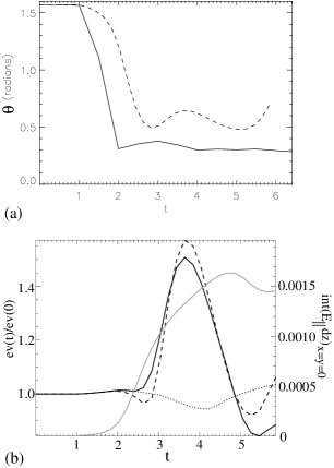
Figure 7: (a) Evolution of the angle ($\theta$) between the spine and fan (eigenvectors), for continual driving with parameters as in Fig. 6 (solid line) and the transient driving run (dashed). (b) Evolution of the null point eigenvalues ($x$-eigenvalue solid line, $y$ dashed, $z$ dotted), and the integrated parallel electric field along the $z$-axis (grey) for the transient driving run. The eigenvalues are normalised to their values at $t=0$, for clarity.

III.4 Parallel electric field and reconnection

Further indications that non-ideal processes are important at the null are given by the presence of a component of ${\bf E}$ parallel to ${\bf B}$ ($E_{\|}$) which develops there. The presence of a current sheet at the null, together with a parallel electric field, is a strong indication that reconnection is taking place in the vicinity of the null (we actually expect that field lines change their connectivity everywhere within the volume defined by the current sheet (the ‘diffusion region’), not only at the null itself Priest et al. (2003); Pontin et al. (2005), which is special only in that the footpoint mapping is discontinuous there).

It can be shown (Pontin et al., 2005) that $\Psi=\displaystyle\int_{x=y=0}E_{\|}\>dz$ provides a measure of the reconnection rate at the null. This quantity gives an exact measure of the rate of flux transfer across the fan surface when the non-ideal region is localised around the null point. The spatial distribution of $E_{\|}$ within the domain when it reaches its temporal maximum is closely focused around the $z$-axis (see Fig. 8). This is because ${\bf J}\|{\bf B}$ there by symmetry (note also that $E_{\|}$ is discontinuous at the plane $z=0$ by symmetry, since $B_{z}$ changes sign through this plane but $J_{z}$ (and thus $E_{z}$) is uni-directional—however, $\displaystyle\int E_{\|}\>ds$ is non-zero since $ds$ also changes sign through $z=0$). The field line which is coincident with the $z$-axis (by symmetry) thus provides the maximum value for $\displaystyle\int E_{\|}\>ds$ of any field line threading the current sheet—another reason to associate this quantity with the reconnection rate.

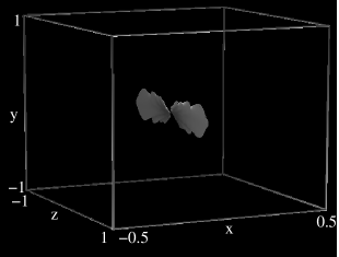
Figure 8: Isosurface of $E_{\|}$ at $t=4.75$ (time of its maximum), at $65\%$ of maximum, transient driving run.

The nature of the field line reconnection can be studied by integrating field lines threading ‘trace particles’, which move in the ideal flow far from the current sheet, and which initially define coincident sets of field lines (see Fig. 9). Once the current sheet forms, field lines traced from particles far out along the spine and far out along the fan are no longer coincident (i.e. they have been ‘reconnected’, near the null). Field lines traced from around the spine flip around the spine, while there is also clearly advection of magnetic flux across the fan surface. However, it seems that this occurs in the main part during the collapse of the null, while later in the simulations reconnection around/through the spine is dominant, since the boundary driving is across the spine.

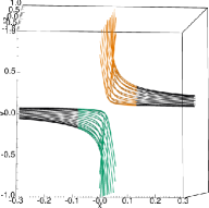
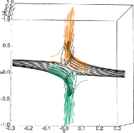
(a) (b) (c)

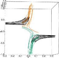
Figure 9: (Colour online) Field lines integrated from ideal trace particles, located initially far out along the spine (black) and the fan (grey, green and orange online). Images for (a) $t=0$, (b) $t=3$, (c) $t=6$, and for continual driving with parameters as in Fig. 6, but $v_{0}=0.03$.

IV Quantitative current sheet properties

In order to understand the nature of the current sheet that forms at the null point, its quantitative properties should be analysed. We focus here on two main aspects, firstly the scaling of the current sheet with the driving velocity, and secondly its behaviour at large times under continual driving. Crucial in this is whether the behaviour tends towards that of a Sweet-Parker-type current sheet, that is whether the sheet’s length increases eventually to system-size, and whether the peak reconnection rate scales as a negative power of $\eta$, thus providing only slow reconnection for small $\eta$. While the computational cost of a scaling study of $J_{max}$ with $\eta$ for a fully 3D simulation such as ours is prohibitive, the investigations which we do perform provide an indication of the nature of the sheet.

IV.1 Scaling with $v_{0}$

Firstly we consider the scaling of the current sheet with the magnitude of the boundary driving velocity. In particular, we look at the maximum current density which is attained (which invariably occurs at the null), the maximum reconnection rate (calculated as the integrated parallel electric field along the fan field line coincident with the $z$-axis, as described previously), and also the current sheet dimensions $L_{x}$, $L_{y}$ and $L_{z}$ (taken to be the full width at half maximum in each coordinate direction). This is done for the case of transient driving, with $\tau$ fixed at a value of $1.8$.

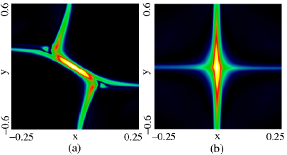
Figure 10: (Colour online) Current modulus in the $z=0$ plane at time of current maximum, for (a) $v_{0}=0.04$, (b) $v_{0}=0.001$, scaled in each case to the individual maximum (20.4 in (a) and 0.44 in (b)).

One point which should be taken into account when considering the measurements of the dimensions of the current sheet (particularly in the $x$- and $y$-directions), is that the measurements do not necessarily mean exactly the same thing in the different simulation runs, in the sense that the current sheet morphology is not always qualitatively the same. Observe the difference between the current structures in Fig. 10, which shows cases with different driving strengths. When the driving in stronger, the current sheet is more strongly focused, and we measure a straight current sheet, which spans the spine and fan [Fig. 10(a)]. However, when the driving is weaker, the region of high (above one half maximum) current density spreads along the fan plane, in an ‘S’ shape in and $xy$-plane [Fig. 5(c)]. Finally, when $v_{0}$ is decreased further still, we again have an approximately planar current sheet, but this time lying in the fan plane [Fig. 10(b)]. Note that this changing morphology is also affected by the parameters $\eta$, $\beta$ and $\gamma$, which we will discuss in a future paper, but which are held fixed here.

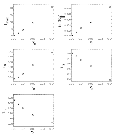
Figure 11: Scaling with the modulus of the driving velocity ($v_{0}$) of the peak current ($J_{max}$), the peak reconnection rate ($\int E_{\|}$), and the full width at half maximum of the current sheet in each coordinate direction ($L_{x},L_{y},L_{z}$).

We repeat the simulations with transient driving, varying $v_{0}$, but fixing $X_{l}=0.5$, $Y_{l}=Z_{l}=3$, $A_{d}=80$, $\tau=1.8$ and $\eta=5\times 10^{-4}$. The results are shown in Fig. 11. First, we see that the peak current and peak reconnection rate both scale linearly with $v_{0}$. The extent of the current sheet in $x$ ($L_{x}$) increases linearly with $v_{0}$, which is a signature of the increased collapse of the null. By contrast, $L_{y}$ decreases with increased driving velocity. This is rather curious and seems counter-intuitive. It appears that the current sheet is more intense and more strongly focused at the null for stronger driving. In addition though, it is a result of the fact that an increasing amount of the current is able to be taken up in a straight spine-fan spanning current sheet, rather than spreading in the fan plane. Likewise the scaling of $L_{z}$ is also curious—the current sheet is more intense and strongly focused at the null for stronger driving.

The above scaling analysis has also been performed for the case where the spine is displaced by the same amount each time, but at different rates. That is, as $v_{0}$ is increased, $\tau$ is decreased to compensate. In fact the scaling results are very similar to those above, but just with a slightly weaker dependence on $v_{0}$.

IV.2 Long-time growth under continual driving

Now consider the case where, rather than imposing the boundary driving for only a limited time, the driving velocity is ramped up and then held constant. We take parameters as in Sec. III.1, but with $Y_{l}=Z_{l}=6$ and run resolution $128\times 192\times 192$, giving minimum $\delta x\sim 0.005$ and $\delta y,\delta z\sim 0.025$ again at the null. We focus on whether the current sheet continues to grow when it is continually driven, or whether it reaches a fixed length due to some self-limiting mechanism. As before, one of the major issues we run into between different simulation runs which use different parameters is in the geometry of the current sheet. For simplicity here we consider a case with sufficiently strong driving that the current sheet is approximately straight, spanning the spine and fan, as in Fig. 10(a).

There are many problems which make it hard to determine the time evolution of the current sheet length. During the initial stage of the sheet formation, it actually shrinks, as it intensifies, in the $xy$-plane (measuring the length as $\sqrt{L_{x}^{2}+L_{y}^{2}}$, see Fig. 12(a)). After this has occurred, the sheet then grows very slowly—differences over an Alfvén time are on the order of the gridscale. There is no sign though of any evidence which points to a halting of this growth. Similarly, examining the evolution of $L_{z}$, it seems to continue increasing for as long as we can run the simulations. Neither of the above is controlled by the dimensions of the numerical domain (see Fig. 12(b)).

(a) (b) (c)

Figure 12: Growth of the sheet in time, in (a) the $xy$-direction ($\sqrt{L_{x}^{2}+L_{y}^{2}}$) and (b) the $z$-direction for three runs with different domain sizes ($Y_{l}=Z_{l}=6$ solid line, $Y_{l}=Z_{l}=3$ dashed, $Y_{l}=Z_{l}=1.5$ dot-dashed). (c) Time evolution of the maximum value of each current component ($J_{x}$ solid line, $J_{y}$ dotted, $J_{z}$ dashed.)

As to the value of the peak current, and the reconnection rate at the null, though the growth of these slows significantly as time progresses (see Fig. 12(c)), there is again no sign of them reaching a saturated value. The slowing of the current sheet growth (dimensions and modulus) is undoubtedly down to the diffusion and reconnection which occurs in the current sheet.

In summary, it is difficult to be definitive that the current sheet will grow to system-size under continuous driving, due to the computational difficulties of running for a long time. However, there is no indication that the dimensions of the current sheet are limited by any self-regulating process. Rather, the dimensions are determined by the boundary conditions (i.e. the degree of shear imposed from the driving boundaries at a given time). Thus, if it were computationally possible to continue the shearing indefinitely, it appears that the sheet would continue to grow in size and intensity. If the system size is large and the resistivity is low, it is possible that the extended current sheet may break up into secondary islands, which lie beyond the scope of the present simulations.

V Possibility of turbulent reconnection

A crucial aspect of any reconnection model which hopes to explain fast energy release is the scaling of the reconnection rate with the dissipation parameter. Mechanisms for turbulent reconnection have been put forward which predict reconnection rates which are completely independent of the resistivity Lazarian and Vishniac (1999). Recent work by Eyink and Aluie Eyink and Aluie (2006), who obtain conditions under which Alfvén’s “frozen flux” theorem may be violated in ideal plasmas, has placed rigourous constraints on models of turbulent reconnection. The breakdown of Alfvén’s theorem occurs over some length scale defined by the turbulence, which may be much larger than typical dissipative length scales. Eyink and Aluie demonstrate that in such a turbulent plasma, a necessary condition for such a breakdown to occur is that current and vortex sheets intersect one another . This is a rather strong condition on the nonlinear dynamics underlying a turbulent MHD plasma. (Note that in order to correspond to any type of reconnection geometry, more than two current/vortex sheets should intersect, or equivalently they should each have multiple ‘branches’, as in Fig. 13, say along the separatrices. This ensures a non-zero electric field at the intersection point, unlike in the simplified example of Eyink and Aluie.)

One possible viewpoint of how such a situation might occur is that these current sheets and vortex sheets are generated by the turbulent mechanism itself. Alternatively, one might imagine another situation in which the result might be applicable is in a configuration where macro-scale current sheets and vortex sheets are present in the laminar solution, which may then be modulated by the presence of turbulence. The results discussed in the previous sections point towards 3D null points as sites where this might occur.

Firstly, examining the vorticity (${\bf\omega}$) profile in the simulations, we find that in fact a highly localised region of strong vorticity is indeed present. Furthermore, this region intersects with the region of high current density (see Fig. 13) and is focused at the null (and possibly spread along the fan surface as described above, depending on the choice of parameters).

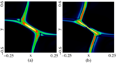
Figure 13: (Colour online) (a) Current and (b) vorticity profiles in the $z=0$ plane through the null, at the time of peak current, for parameters as in Sec. IV.1, with $v_{0}=0.04$.

It also appears from the figure that in fact the vorticity profile forms in narrower layers than the current (in the $xy$-plane), one focused along the spine, with a much stronger layer in the fan (while the current sheet spans the spine and fan), so that rather than being completely coincident, the ${\bf J}$ and ${\bf\omega}$ sheets really do ‘intersect’. The rates at which ${\bf J}$ and ${\bf\omega}$ fall off in $z$ away from the null are also very similar.

Moreover, we have seen in Sec. II.2 that in order for a null point to evolve in certain ways, non-ideal processes are required. When the ideal system is supposed to evolve in such a way, a non-smooth velocity profile results, which typically shows up along either the spine or fan of the null, or both, depending on the boundary conditions. This non-smooth velocity corresponds to a singular vortex sheet.

Finally, it is worth noting that in non-laminar magnetic fields, 3D nulls are expected to cluster together, creating ‘bunches’ of nulls Albright (1999), thus providing the possibility that multiple coincident current and vortex sheets might be closely concentrated.

VI Summary

We have investigated the nature of the MHD evolution, and current sheet formation, at 3D magnetic nulls. In complex 3D fields, isolated nulls are often considered less important sites of energetic phenomena than separator lines, due to the viewpoint that ideal MHD singularities in kinematic analyses are a result of the choice of boundary conditions. However, as demonstrated here (and proven in Ref. [Hornig and Schindler, 1996]), certain evolutions of a 3D null are prohibited under ideal MHD, specifically those which correspond to a time dependence in the eigenvalue ratios of the null. We presented a particular example which demonstrates this, for the case where the angle between the spine and fan changes in time. The flow which advects the magnetic flux in the chosen example is shown to be non-smooth at the spine and/or fan for any choice of external boundary conditions. For typical boundary conditions (as required by say a line-tied boundary such as the solar photosphere, or at another null in the system) the flow will be singular. Thus non-ideal processes are always required to facilitate such an evolution. We presented the results of resistive MHD simulations which demonstrated that this evolution is a generic one.

We went on to investigate the process of current sheet formation at such a 3D null in the simulations. The null was driven by shearing motions at the spine boundary, and a strong current concentration was found to result, focused at the null. The spine and fan of the null close up on one another, from their initial orthogonal configuration. Depending on the strength of the driving, the current sheet may be either spread along the fan of the null, or almost entirely contained in a spine-fan spanning sheet (for stronger driving). The structure of the sheet is of exactly anti-parallel field lines in the shear plane at the null, with the intensity of ${\bf J}$ falling off in the perpendicular direction due to the linearly increasing field component in that direction, which is continuous across the current sheet. Repeating our simulations but driving at the fan footpoints instead of the spine, a very similar evolution is observed. The current is still inclined to spread along the fan rather than the spine for weaker driving, consistent with relaxation simulation results Pontin and Craig (2005). This is natural due to the shear driving, and the disparity in the structures of the spine and fan. The spine is a single line to which field lines converge, and the natural way to form a current sheet there is to have those field lines spiral tightly around the spine line. This field structure however is synonymous with a current directed parallel to the spine, and is known to be induced by rotational motions, rather than shearing ones Pontin and Galsgaard (2007).

In addition to the current sheet at the null, indications that non-ideal processes and reconnection should take place there are given by the presence of a localised parallel electric field. The maxima of this parallel electric field occur along the axis perpendicular to the shear ($z$). The integral of $E_{\|}$ along the field line which is coincident with this axis (by symmetry) gives the reconnection rate Pontin et al. (2005), which grows to a peak value in time before falling off after the driving is switched off. Field lines are reconnected both across the fan and around the spine as the null collapses.

As to the quantitative properties of the current sheet, its intensity and dimensions are linearly dependent on the modulus of the boundary driving. In addition, under continual driving, we find no indications which suggest that the sheet does not continue to grow (in intensity and length) in time. That is, its length does not appear to be controlled by any self-regulating mechanism. Rather, its dimensions at a given time are dependent on the boundary conditions (the degree of shearing).

Finally, with respect to a recent theorem of Eyink and Aluie Eyink and Aluie (2006), our results suggest 3D nulls as a possible site of turbulent reconnection. Their theorem states that turbulent reconnection may occur at a rate independent of the resistivity only where current sheets and vortex sheets intersect one another. We find that strong vorticity concentrations are in fact present in our simulations, and are localised at the null and clearly intersect the current sheet. Moreover, in the ideal limit, our kinematic model demonstrates that as the spine and fan collapse towards one another, the vorticity at the fan (or spine, or both) must be singular (due to the non-smooth transport velocity).

VII Acknowledgements

The authors wish to acknowledge fruitful discussions with G. Hornig and C-. S. Ng. This work was supported by the Department of Energy, Grant No. DE-FG02-05ER54832, by the National Science Foundation, Grant Nos. ATM-0422764 and ATM-0543202 and by NASA Grant No. NNX06AC19G. K. G. was supported by the Carlsberg Foundation in the form of a fellowship. Computations were performed on the Zaphod Beowulf cluster which was in part funded by the Major Research Instrumentation program of the National Science Foundation, grant ATM-0424905.

References

- Longcope (1996) D. W. Longcope, Solar Phys. 169, 91 (1996).
- Priest et al. (2005) E. R. Priest, D. W. Longcope, and J. F. Heyvaerts, Astrophys. J. 624, 1057 (2005).
- Priest and Forbes (2000) E. R. Priest and T. G. Forbes, Magnetic reconnection: MHD theory and applications (Cambridge University Press, Cambridge, 2000).
- Siscoe (1988) G. L. Siscoe, Physics of Space Plasmas (Sci. Publ. Cambridge, MA, 1988), pp. 3–78.
- Schrijver and Title (2002) C. J. Schrijver and A. M. Title, Solar Phys. 207, 223 (2002).
- Longcope et al. (2003) D. W. Longcope, D. S. Brown, and E. R. Priest, Phys. Plasmas 10, 3321 (2003).
- Close et al. (2005) R. M. Close, C. E. Parnell, and E. R. Priest, Solar Phys. 225, 21 (2005).
- Fletcher et al. (2001) L. Fletcher, T. R. Metcalf, D. Alexander, D. S. Brown, and L. A. Ryder, Astrophys. J. 554, 451 (2001).
- Aulanier et al. (2000) G. Aulanier, E. E. DeLuca, S. K. Antiochos, R. A. McMullen, and L. Golub, Astrophys. J. 540, 1126 (2000).
- Ugarte-Urra et al. (2007) I. Ugarte-Urra, H. P. Warren, and A. R. Winebarger (2007), the magnetic topology of coronal mass ejection sources, Astrophys. J., in press.
- Xiao et al. (2006) C. J. Xiao, X. G. Wang, Z. Y. Pu, H. Zhao, J. X. Wang, Z. W. Ma, S. Y. Fu, M. G. Kivelson, Z. X. Liu, Q. G. Zong, et al., Nature Physics 2, 478 (2006).
- Bogdanov et al. (1994) S. Y. Bogdanov, V. B. Burilina, V. S. Markov, and A. G. Frank, JETP Lett. 59, 537 (1994).
- Lau and Finn (1990) Y. T. Lau and J. M. Finn, Astrophys. J. 350, 672 (1990).
- Priest and Titov (1996) E. R. Priest and V. S. Titov, Phil. Trans. R. Soc. Lond. A 354, 2951 (1996).
- Bulanov and Olshanetsky (1984) S. V. Bulanov and M. A. Olshanetsky, Phys. Lett. 100, 35 (1984).
- Pontin and Craig (2005) D. I. Pontin and I. J. D. Craig, Phys. Plasmas 12, 072112 (2005).
- Longcope and Cowley (1996) D. W. Longcope and S. C. Cowley, Phys. Plasmas 3, 2885 (1996).
- Fukao et al. (1975) S. Fukao, M. Ugai, and T. Tsuda, Rep. Ion. Sp. Res. Japan 29, 133 (1975).
- Parnell et al. (1996) C. E. Parnell, J. M. Smith, T. Neukirch, and E. R. Priest, Phys. Plasmas 3, 759 (1996).
- Hornig and Priest (2003) G. Hornig and E. R. Priest, Phys. Plasmas 10, 2712 (2003).
- Priest et al. (2003) E. R. Priest, G. Hornig, and D. I. Pontin, J. Geophys. Res. 108, SSH6 (2003).
- Boozer (2002) A. H. Boozer, Phys. Rev. Lett. 88, 215005 (2002).
- Greene (1993) J. M. Greene, Phys. Fluids B 5, 2355 (1993).
- Hornig and Schindler (1996) G. Hornig and K. Schindler, Phys. Plasmas 3, 781 (1996).
- Pontin and Galsgaard (2007) D. I. Pontin and K. Galsgaard, J. Geophys. Res. 112, A03103 (2007).
- Galsgaard and Nordlund (1997) K. Galsgaard and A. Nordlund, J. Geophys. Res. 102, 231 (1997).
- Archontis et al. (2004) V. Archontis, F. Moreno-Insertis, K. Galsgaard, A. Hood, and E. O’Shea, Astron. Astrophys. 426, 1074 (2004).
- Craig and Fabling (1996) I. J. D. Craig and R. B. Fabling, Astrophys. J. 462, 969 (1996).
- Pontin et al. (2004) D. I. Pontin, G. Hornig, and E. R. Priest, Geophys. Astrophys. Fluid Dynamics 98, 407 (2004).
- Green (1965) R. M. Green, in IAU Symp. 22: Stellar and Solar Magnetic Fields (Amsterdam: North-Holland, 1965), p. 398.
- Syrovatskii (1971) S. I. Syrovatskii, Sov. Phys. JETP 33, 933 (1971).
- Pontin et al. (2005) D. I. Pontin, G. Hornig, and E. R. Priest, Geophys. Astrophys. Fluid Dynamics 99, 77 (2005).
- Lazarian and Vishniac (1999) A. Lazarian and E. T. Vishniac, Astrophys. J. 517, 700 (1999).
- Eyink and Aluie (2006) G. L. Eyink and H. Aluie, Physica D 223, 82 (2006).
- Albright (1999) B. J. Albright, Phys. Plasmas 6, 4222 (1999).