Destabilisation of hydrodynamically stable rotation laws by azimuthal magnetic fields

Abstract

We consider the effect of toroidal magnetic fields on hydrodynamically stable Taylor-Couette differential rotation flows. For current-free magnetic fields a nonaxisymmetric $m=1$ magnetorotational instability arises when the magnetic Reynolds number exceeds $O(100)$. We then consider how this ‘azimuthal magnetorotational instability’ (AMRI) is modified if the magnetic field is not current-free, but also has an associated electric current throughout the fluid. This gives rise to current-driven Tayler instabilities (TI) that exist even without any differential rotation at all. The interaction of the AMRI and the TI is then considered when both electric currents and differential rotation are present simultaneously. The magnetic Prandtl number Pm turns out to be crucial in this case. Large Pm have a destabilizing influence, and lead to a smooth transition between the AMRI and the TI. In contrast, small Pm have a stabilizing influence, with a broad stable zone separating the AMRI and the TI. In this region the differential rotation is acting to stabilize the Tayler instabilities, with possible astrophysical applications (Ap stars). The growth rates of both the AMRI and the TI are largely independent of Pm, with the TI acting on the timescale of a single rotation period, and the AMRI slightly slower, but still on the basic rotational timescale. The azimuthal drift timescale is $\sim 20$ rotations, and may thus be a (flip-flop) timescale of stellar activity between the rotation period and the diffusion time.

1 Introduction

We consider the problem of how linear hydrodynamic and magnetohydrodynamic instabilities interact in a simple rotating shear flow, the familiar Taylor-Couette flow between concentric cylinders. In the purely hydrodynamic problem, the Rayleigh criterion states that an ideal flow is stable against axisymmetric perturbations when the specific angular momentum increases outwards

$$\frac{\rm d}{{\rm d}R}(R^{2}\Omega)^{2}>0,$$ (1)

where $\Omega$ is the angular velocity, and cylindrical coordinates ($R$, $\phi$, $z$) are used. Viscosity has a stabilizing effect, so that a Taylor-Couette flow that violates (1) becomes unstable only if the angular velocity of the inner cylinder (that is, its Reynolds number) exceeds some critical value.

If a uniform axial magnetic field is included, a new type of instability arises, the magnetorotational instability (MRI). The Rayleigh criterion is then replaced by

$$\frac{\rm d}{{\rm d}R}\Omega^{2}>0.$$ (2)

That is, the requirement for stability is that the angular velocity itself increases outward, rather than the angular momentum. This is more stringent than (1), so a flow may be hydrodynamically stable, but magnetohydrodynamically unstable. And again, viscosity and/or magnetic diffusivity have a stabilizing effect; for small magnetic Prandtl numbers it is the magnetic Reynolds number that must exceed a critical value for instability to occur (Rüdiger, Schultz & Shalybkov 2003). Hollerbach & Rüdiger (2005) considered how the magnetorotational instability is modified if an azimuthal field $B_{\phi}\propto R^{-1}$ is added, and found that the relevant parameter is then the ordinary Reynolds number $\rm Re$, rather than the magnetic Reynolds number $\rm Rm$.

In this work we will consider instabilities of purely azimuthal magnetic fields, without any axial field being present. We begin by showing that even $B_{\phi}\propto R^{-1}$ by itself supports a magnetorotational instability. This new type of MRI is nonaxisymmetric, having azimuthal wavenumber $m=1$, but otherwise shares all the characteristics of the classical, axisymmetric MRI in an axial field. These results are presented in section 3.

We then extend the choice of imposed field to be of the form $B_{\phi}=a_{B}R+b_{B}R^{-1}$. The part $b_{B}R^{-1}$ corresponds to an axial current only within the inner cylinder $R<R_{\rm{in}}$, so current-free within the fluid, but the part $a_{B}R$ corresponds to a uniform axial current density $J_{z}=2a_{B}$ everywhere within $R<R_{\rm{out}}$. Taking $B_{\phi}=a_{B}R+b_{B}R^{-1}$ instead of just $B_{\phi}=b_{B}R^{-1}$ has profound implications, well beyond simply having a somewhat different radial profile. In particular, if there are no electric currents flowing within the fluid ($a_{B}=0$), the only source of energy to drive instabilities is the differential rotation; the magnetic field merely acts as a catalyst, not as a source of energy. For $\rm Re=0$ no instabilities are thus possible, regardless of how strong the magnetic field is.

In contrast, if there are electric currents flowing within the fluid ($a_{B}\neq 0$), this yields a new source of energy to drive purely magnetic instabilities, that may exist even at $\rm Re=0$. Michael (1954) and Velikhov (1959) considered axisymmetric magnetic instabilities and derived the stability criterion

$$\frac{\rm d}{{\rm d}R}\left(\frac{B_{\phi}}{R}\right)^{2}<0.$$ (3)

Tayler (1973) included nonaxisymmetric disturbances and showed that for an ideal fluid the necessary and sufficient condition for stability is

$$\frac{\rm d}{{\rm d}R}(RB_{\phi}^{2})<0.$$ (4)

A uniform field would therefore be axisymmetrically stable, but nonaxisymmetrically unstable, with $m=1$ being the most unstable mode. (The profile $B_{\phi}\propto R^{-1}$ is stable according to both (3) and (4), in agreement with the discussion above, that for such a current-free profile there is simply no source of energy to drive purely magnetic instabilities.)

In section 4 we then choose $a_{B}$ and $b_{B}$ such that $B_{\phi}$ is as uniform as possible, with the same values at $R_{\rm in}$ and $R_{\rm out}$. We consider how the resulting Tayler instabilities (TI) interact with the azimuthal magnetorotational instabilities (AMRI) presented in section 3. We find that the magnetic Prandtl number plays a key role: if $\rm Pm\lower 1.72218pt\hbox{$\;\buildrel>\over{\scriptstyle\sim}\;$}10$ the AMRI and the TI are smoothly connected to one another, but if $\rm Pm\lower 1.72218pt\hbox{$\;\buildrel<\over{\scriptstyle\sim}\;$}1$ they are disconnected, with a region of stability separating them.

The results presented here have important astrophysical implications, since the simultaneous existence of differential rotation and toroidal magnetic fields is characteristic of almost all celestial bodies. Prominent examples of differentially rotating objects with large magnetic Prandtl number are protogalaxies (without supernova explosions) and protoneutron stars (PNS). Even rather weak toroidal fields should be unstable in these objects. In contrast, the radiative zones of stars have $\rm Pm<10^{-2}$. In this case we will see that the toroidal field is stabilized, as long as it is not too strong. Finally, in the limit of no differential rotation, the pure Tayler instability is independent of $\rm Pm$.

2 Basic equations

We consider a viscous, electrically conducting, incompressible fluid between two rotating infinite cylinders, in the presence of an azimuthal magnetic field. The equations of the problem are

$$\frac{\partial\mbox{\boldmath$U$}}{\partial t}+(\mbox{\boldmath$U$}\cdot\nabla)\mbox{\boldmath$U$}=-\frac{1}{\rho}\nabla P+\nu\Delta\mbox{\boldmath$U$}+\frac{1}{\mu_{0}\rho}{\mathop{\rm rot}\nolimits\mbox{\boldmath$B$}}\times\mbox{\boldmath$B$},$$

$$\frac{\partial\mbox{\boldmath$B$}}{\partial t}={\mathop{\rm rot}\nolimits}\ (\mbox{\boldmath$U$}\times\mbox{\boldmath$B$})+\eta\Delta\mbox{\boldmath$B$},$$ (5)

and

$${\mathop{\rm div}\nolimits}\ \mbox{\boldmath$U$}={\mathop{\rm div}\nolimits}\ \mbox{\boldmath$B$}=0,$$ (6)

where $U$ is the velocity, $B$ the magnetic field, $P$ the pressure, $\nu$ the kinematic viscosity, and $\eta$ the magnetic diffusivity. Equations (5) yield the basic state solution

$$U_{R}=U_{z}=B_{R}=B_{z}=0,$$ (7)

and

$$U_{\phi}=R\Omega=a_{\Omega}R+\frac{b_{\Omega}}{R},\qquad B_{\phi}=a_{B}R+\frac{b_{B}}{R}.$$ (8)

$a_{\Omega}$ and $b_{\Omega}$ are given by

$$a_{\Omega}=\Omega_{\rm{in}}\frac{\hat{\mu}_{\Omega}-{\hat{\eta}}^{2}}{1-{\hat{\eta}}^{2}},\qquad b_{\Omega}=\Omega_{\rm{in}}R_{\rm{in}}^{2}\frac{1-\hat{\mu}_{\Omega}}{1-{\hat{\eta}}^{2}},$$ (9)

where

$$\hat{\eta}=\frac{R_{\rm{in}}}{R_{\rm{out}}},\qquad\hat{\mu}_{\Omega}=\frac{\Omega_{\rm{out}}}{\Omega_{\rm{in}}}.$$ (10)

$\Omega_{\rm in}$ and $\Omega_{\rm out}$ are the imposed rotation rates of the inner and outer cylinders, with radii $R_{\rm in}$ and $R_{\rm out}$.

In contrast to $U_{\phi}$, where $a_{\Omega}$ and $b_{\Omega}$ are merely derived quantities ($\Omega_{\rm in}$ and $\Omega_{\rm out}$ being the fundamental quantities), for $B_{\phi}$, $a_{B}$ and $b_{B}$ themselves are the fundamental quantities; as previously noted, $a_{B}R$ corresponds to a uniform axial current everywhere within $R<R_{\rm out}$, and $b_{B}R^{-1}$ corresponds to an additional current only within $R<R_{\rm in}$. In analogy with $\hat{\mu}_{\Omega}$, it is useful though to define the quantity

$$\hat{\mu}_{B}=\frac{B_{\rm{out}}}{B_{\rm{in}}}=\frac{a_{B}R_{\rm out}+b_{B}R_{\rm out}^{-1}}{a_{B}R_{\rm in}+b_{B}R_{\rm in}^{-1}},$$ (11)

measuring the variation in $B_{\phi}$ across the gap.

In section 3 we consider the field $B_{\phi}\propto R^{-1}$, so $a_{B}=0$ and $b_{B}=1$. In contrast, in section 4 we include nonzero $a_{B}$, and adjust it so that $\hat{\mu}_{B}=1$, so the toroidal field profile is as uniform as possible (see also Cally 2003). Taking $R_{\rm in}=1$ and $R_{\rm out}=2$, this corresponds to setting $a_{B}=1/3$ and $b_{B}=2/3$; $B_{\phi}$ then varies by less than 6% across the gap.

We are interested in the linear stability of the solution (8). The perturbed state of the flow is described by

$$u_{R},\;R\Omega+u_{\phi},\;u_{z},\;b_{R},\;B_{\phi}+b_{\phi},\;b_{z}.$$ (12)

Developing the disturbances into normal modes, solutions of the linearized equations are considered in the form

$$F=F(R){\rm{exp}}\bigl{[}{\rm{i}}(kz+m\phi+\omega t)\bigr{]},$$ (13)

where $F$ is any of the perturbation quantities.

The magnetic Prandtl number (Pm), the Hartmann number (Ha) and the Reynolds number (Re) are the dimensionless numbers of the problem,

$${\rm{Pm}}=\frac{\nu}{\eta},\qquad\ {\rm{Ha}}=\frac{B_{\rm{in}}R_{0}}{\sqrt{\mu_{0}\rho\nu\eta}},\qquad\ {\rm{Re}}=\frac{\Omega_{\rm{in}}R_{0}^{2}}{\nu},$$ (14)

where $R_{0}=(R_{\rm{in}}(R_{\rm{out}}-R_{\rm{in}}))^{1/2}$ is taken as the unit of length. We have used $R_{0}^{-1}$ as the unit of the wave number, $\eta/R_{0}$ as the unit of the velocity fluctuations, $\Omega_{\rm{in}}$ as the unit of frequencies, and $B_{\rm{in}}$ as the unit of the magnetic field fluctuations. Where appropriate, we will also use the magnetic Reynolds number

$$\rm Rm=Pm\cdot Re$$ (15)

and the Lundquist number

$$\rm S=\sqrt{Pm}\cdot Ha.$$ (16)

A set of ten boundary conditions is needed to solve the equations, namely no-slip

$$u_{R}=u_{\phi}=u_{z}=0$$ (17)

for the flow, and perfectly conducting

$${\rm d}b_{\phi}/{\rm d}R+b_{\phi}/R=b_{R}=0$$ (18)

for the field, both sets being applied at both $R_{\rm{in}}$ and $R_{\rm{out}}$. If the exterior regions were taken to be insulators, the boundary conditions on the field would be different (e.g. Rüdiger, Schultz & Shalybkov 2003; Shalybkov 2006), but here we will consider only conducting boundary conditions.

The system of linearized equations and associated boundary conditions then constitutes a one-dimensional linear eigenvalue problem, solved by finite-differencing in radius as in Rüdiger et al. (2005). Typically around 100 grid points were used, and all results were checked to ensure that they were fully resolved.

3 The azimuthal magnetorotational instability (AMRI)

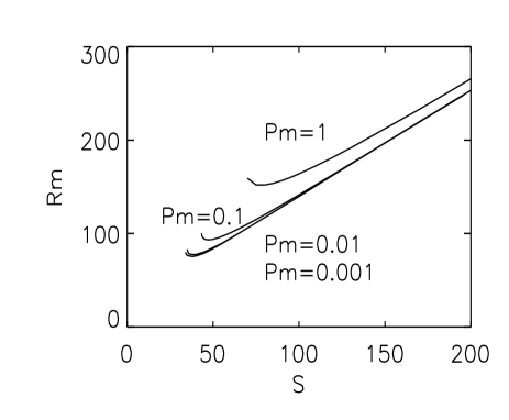
Figure 1: The marginal stability domains for the $m=1$ azimuthal magnetorotational instability (AMRI) with $\hat{\eta}=0.5$ conducting cylinders. The outer cylinder rotates with 50% of the rotation rate of the inner one, $\hat{\mu}_{\Omega}=0.5$; the magnetic field between the cylinders is current-free, $\hat{\mu}_{B}=0.5$. The curves are marked with their magnetic Prandtl numbers.

The rotation laws in stars and galaxies are hydrodynamically stable. Such rotation laws can be modeled by Taylor-Couette containers with rotating outer cylinder. More precisely, the rotation of the outer cylinder must fulfill the Rayleigh condition, $\hat{\mu}>\hat{\eta}^{2}$. The containers considered here have $\hat{\eta}=0.5$, so that a flow with $\hat{\mu}=0.5$ is clearly beyond the Rayleigh limit where the hydrodynamic instability disappears. Such a rotation law, however, can become unstable against nonaxisymmetric disturbances under the presence of a current-free toroidal field. Figure 1 shows stability curves for $m=1$, the only mode that appears to become unstable. We see how a magnetorotational instability exists that is remarkably similar to the classical MRI with a purely axial field. In particular, as ${\rm Pm}\to 0$, the relevant parameters are also $\rm Rm$ and $\rm S$, with the MRI arising if ${\rm Rm}\lower 1.72218pt\hbox{$\;\buildrel>\over{\scriptstyle\sim}\;$}80$, and ${\rm S}\approx 40$ yielding the lowest value of $\rm Rm_{c}$. The specific numbers are roughly an order of magnitude greater than for the axisymmetric MRI in the axial field (cf. Rüdiger, Schultz & Shalybkov 2003), but the basic scalings, and even the detailed shape of the instability curves, are identical.

Figure 2 shows the real and imaginary parts of ${\rm i}\omega$ in the unstable regime. Remembering that time has been scaled by $\Omega_{\rm in}^{-1}$, we see that we obtain growth rates as large as $0.05\Omega_{\rm in}$. So again, while the particular number 0.05 is about an order of magnitude smaller than for the axisymmetric MRI in the axial field, this nonaxisymmetric MRI is clearly also growing on the basic rotational timescale.

Figure 2: The growth rates (top) and azimuthal drift rates (bottom), as functions of $\rm S$, with $\rm Rm$ fixed at 200.

To understand why this nonaxisymmetric MRI exists even for a purely toroidal field ${\mbox{\boldmath$B$}}_{0}$, for which it is known that the axisymmetric MRI fails, we need to consider the $r$ and $\phi$ components of the induction equation,

$${\rm Rm}\,{\rm i}\omega b_{R}=\Delta b_{R}-R^{-2}b_{R}-2{\rm i}mR^{-2}b_{\phi}+$$ (19)

$$\qquad\quad+{\rm i}mR^{-2}u_{R}-{\rm Rm}\,{\rm i}m\Omega\,b_{R},$$

$${\rm Rm}\,{\rm i}\omega b_{\phi}=\Delta b_{\phi}-R^{-2}b_{\phi}+2{\rm i}mR^{-2}b_{R}+$$

$$\ \ \ +{\rm i}mR^{-2}u_{\phi}+2R^{-2}u_{R}-{\rm Rm}\,{\rm i}m\Omega\,b_{\phi}+{\rm Rm}\,R\frac{{\rm d}\Omega}{{\rm d}R}\,b_{R}.$$ (20)

In particular, note that for $m=0$, $b_{R}$ completely decouples from everything else, and inevitably decays away. Without $b_{R}$ though, the MRI cannot proceed, as it relies on the term $R({{\rm d}\Omega}/{{\rm d}R})b_{R}$. In contrast, for $m=1$, $b_{R}$ is coupled both to $b_{\phi}$, coming from $\Delta{\mbox{\boldmath$b$}}$, and to $u_{R}$, from $\mathop{\rm rot}\nolimits(\mbox{\boldmath$u$}\times\mbox{\boldmath$B$}_{0})$. And once $b_{R}$ is coupled to the rest of the problem, the term $R({{\rm d}\Omega}/{{\rm d}R})b_{R}$ then allows the MRI to develop. A detailed examination of the structure of the solutions shows that all three components of both $u$ and $b$ are indeed present.

We emphasize also that this indeed is a magnetorotational instability, and not a pinch, Tayler, or other current-driven instability. Once again, for a current-free field all current-driven instabilities are excluded a priori. What we have here is that a magnetic field, which by itself would be stable at any amplitude, acts as a catalyst and destabilizes a hydrodynamically stable differential rotation, just as in the classical MRI. We note though that there is no hope of realizing this AMRI in the laboratory; not only is the critical magnetic Reynolds number rather large, but beyond that, achieving a sufficiently strong toroidal field would require enormously large electric currents, beyond what could reasonably be imposed.

Figure 3: The marginal stability domains (hatched) for the $m=1$ TI and AMRI together, for $\hat{\eta}=0.5$ conducting cylinders. The outer cylinder rotates with 50% of the rotation rate of the inner one, $\hat{\mu}_{\Omega}=0.5$; the magnetic field between the cylinders is as uniform as possible, $\hat{\mu}_{B}=1$. The panels are marked with their magnetic Prandtl numbers.

4 The Tayler instability (TI)

Having demonstrated that the current-free field $B_{\phi}=R^{-1}$ yields this nonaxisymmetric azimuthal magnetorotational instability, we next wish to consider what effect including currents within the fluid ($a_{B}\neq 0$) has. There are two questions one might wish to address here. First, how robust is the AMRI in this case; does it continue to exist at all, and if so, are the growth and drift rates much the same? Second, as discussed in the introduction, if there are currents flowing within the fluid, then for sufficiently great Hartmann numbers Tayler instabilities exist (here $\rm Ha_{\rm Tayler}\simeq 150$), which also turn out to be $m=1$, and could thus be expected to interact in some significant way with the AMRI. In this section we therefore consider the nature of this interaction between the AMRI and the TI, and in particular how it depends on the magnetic Prandtl number Pm.

Generally, as one can read from Fig. 3 fast rotation is stabilizing and strong toroidal fields are stabilizing (Pitts & Tayler 1985). However, large magnetic Prandtl numbers also prove to be strongly destabilizing (Fig. 3, top). The right half of the AMRI branch, the one for strong magnetic fields, disappears completely. Instead, the critical Rm decreases monotonically with Ha until eventually $\rm Ha_{\rm Tayler}\simeq 150$ is reached. The transition from the AMRI to the TI is smooth, without any striking features.

However, for $\rm Pm\lower 1.72218pt\hbox{$\;\buildrel<\over{\scriptstyle\sim}\;$}1$ the stable right branch of the AMRI in Fig. 1 reappears. There is always a domain between the AMRI and the TI where the flow is stable, despite the large magnetic fields, $\rm Ha>Ha_{\rm Tayler}$), that is, in a regime where the field without a differential rotation would be unstable. Roughly speaking, according to the results in Fig. 3 (bottom), the TI exists for sufficiently strong magnetic field, i.e.

$${\rm S}\gg{\rm Rm}$$ (21)

and the AMRI exists for sufficiently weak magnetic field, i.e.

$${\rm S}\ll{\rm Rm}$$ (22)

(for $\rm Pm\lower 1.72218pt\hbox{$\;\buildrel<\over{\scriptstyle\sim}\;$}1$). With the magnetic velocity $v_{\rm A}=B_{\phi}/\sqrt{\mu_{0}\rho}$ and the linear rotation speed $U_{\phi}=R_{\rm in}\Omega_{\rm in}$ then

$$\frac{v_{\rm A}}{U_{\phi}}\gg\frac{\Delta R}{R}$$ (23)

for TI and

$$\frac{v_{\rm A}}{U_{\phi}}\ll\frac{\Delta R}{R}$$ (24)

for AMRI. Here $\Delta R/R$ is the fractional layer thickness which is of order unity in our model while for the solar tachocline its value is about 0.05. The AMRI and TI are separated by an extended stable domain where $v_{\rm A}/U_{\phi}\approx\Delta R/R$.

For small Pm and for sufficiently high Reynolds number a second (smaller) critical Hartmann number exists so that depending on the initial conditions two different stable solutions are possible. A solution with growing amplitude (e.g. dynamo-induced) becomes unstable already at $\rm Ha\simeq 50$ while a decaying magnetic field (e.g. after collapse) already becomes stable at $\rm Ha>150$.

For our special magnetic-field profile ($\hat{\mu}_{B}=1$) and for sufficiently large Reynolds numbers, the lower critical Hartmann number moves from 150 for small Pm to about 50 for large Pm (see Fig. 3). Large Pm are destabilizing, and small Pm are stabilizing (Kurzweg 1963). However, even for $\rm Pm>100$, we did not find smaller values than $\rm Ha\simeq 50$. This finding is important for objects with very high magnetic Prandtl number like PNS and protogalaxies. They can possess stable toroidal magnetic fields of finite value, up to $\rm Ha\simeq 50$.

Obviously, for very small magnetic Prandtl number the AMRI becomes less and less important. Magnetic fields with $\rm Ha<Ha_{\rm Tayler}$ are stable for almost all Re. For $\rm Ha>Ha_{\rm Tayler}$ this zone of stability separating the AMRI and TI branches plays an important role though. For a broad range of Reynolds numbers even strong magnetic fields are stabilized against the Tayler instability.

5 Growth rates

As we have demonstrated with Fig. 2 (top) the current-free AMRI shown in Fig. 1 has growth rates $\gamma=-\Im({\omega})$ of around $0.05\Omega_{\rm in}$, only very weakly dependent on Pm. To characterize the instabilities with weak currents we compute the complex frequency and the wave number in the instability domain shown in Fig. 3 for two values of Pm and for two particular, sufficiently large Reynolds numbers. On both the limiting magnetic fields, of course, the growth rate vanishes. Its maximal value between both the limits is (here) 0.004 (see Fig. 4). That there is a proportionality $\gamma\propto\rm Ha^{2}$ of the growth rate as suggested by Spruit (1999, his Eq. 37) cannot be confirmed.

Figure 4: The growth rate for the azimuthal magnetorotational instability with weak currents (see Fig. 3) for $\rm Pm=1$ (left, here $\rm Rm=125$) and for $\rm Pm=0.1$ (right, here $\rm Rm=82$).

The resulting growth rate of only 0.004 means that the instability grows with a characteristic time of about 40 rotation periods of the inner cylinder, i.e. for 20 rotation periods of the outer cylinder. It is a rather slow instability. However, the growth rates also depend on the Reynolds number. They are very small close to the marginal stability limit and they grow with growing Reynolds number. For slightly supercritical Reynolds numbers one finds for ${\rm Pm}=1$ the growth rate expression $\gamma\simeq(\rm Re-Re_{\rm crit})/1333$ with $\rm Re_{crit}=119$ (Fig. 5, left). The faster the rotation the faster the growth rate, but there is a saturation of the growth rates, which does not depend strongly on Pm (see Fig. 5, right). The saturation value for $\rm Pm=1$ is about 0.12 and for (the more realistic) $\rm Pm=0.1$ it is about 0.10. This maximum growth rate translates into about 1.5 rotation times of the inner cylinder. Note therefore that the AMRI is a fast instability for turbulent media with their typical value of $\rm Pm\leq 1$, but it may be slower for the laminar gas of radiative stellar cores ($\rm Pm\leq 10^{-{(2\dots 3)}}$).

Figure 5: The growth rate shown in Fig. 4 for growing magnetic Reynolds numbers Rm for $\rm Pm=1$ (left) and $\rm Pm=0.1$ (right). The curves are marked with the Lundquist numbers S for which the growth rates have a maximum.

The main sequence stars of spectral class A as a group are fast rotators with high Reynolds numbers. The magnetic Ap stars are the slower rotators in the group so that they should have smaller Reynolds numbers than the nonmagnetic A stars. Inspecting Fig. 3 (for small magnetic Prandtl number, bottom) one may speculate that the A stars as a group are located at the limit between AMRI and the stability branch. Then the Ap stars would lie in the slow-rotation stable regime while the nonmagnetic A stars would lie in the unstable AMRI regime. Toroidal fields induced by differential rotation of order $10^{7}$ Gauss would then be stable for the slow rotators (Ap) and unstable for the fast rotators (A). It is necessary, however, for this kind of theory of the Ap stars that in Fig. 3 (bottom) the differential-rotation-induced stable domain also exists for sufficiently high Reynolds numbers and Hartmann numbers, which is still unknown (cf. Braithwaite & Spruit 2004).

The TI seems to be faster than the AMRI. The growth rates show that only (say) one rotation time is enough to develop the instability.

Figure 6: The growth rates for $\rm Re=40$ in the TI corner of Fig. 3 (middle, $\rm Pm=1$). Note that the growth rates for TI are higher than for AMRI and that they vary linearly with the magnetic field.

The growth rate presented in Fig. 6 scales linearly with the magnetic field. This result clearly confirms the early finding of Goossens, Biront & Tayler (1981) who found for nonrotating stars with toroidal fields the relation

$$\gamma\lower 1.72218pt\hbox{$\;\buildrel>\over{\scriptstyle\sim}\;$}\frac{B_{\phi}}{\sqrt{\mu_{0}\rho}R}$$ (25)

for the growth rate. Translated to our notation this might mean

$$\frac{\gamma}{\Omega}\lower 1.72218pt\hbox{$\;\buildrel>\over{\scriptstyle\sim}\;$}\frac{\rm Ha}{\rm Re\sqrt{Pm}},$$ (26)

leading to values exceeding unity in accordance to their numerical results (their Table 1). For a typical A star Goossens & Veugelen (1978) find $50\dots 500$ days. The values in Fig. 6 which we obtained under the presence of rotation are of the same order, leading to growth times of one rotation period.

6 Azimuthal drift

For almost all nonaxisymmetric phenomena there is an azimuthal drift of the pattern $\dot{\phi}=-\Re(\omega)/m$. Negative (positive) real parts of the frequency $\omega$, therefore, means eastward (westward) migration. If the pattern is considered in the system corotating with the outer cylinder the value 0.5 must be added, which has already been done in Figs. 7 and 8. Then the resulting normalized drift is $-0.05$ in units of the outer rotation, or $-0.025$ in units of the inner rotation. The negative sign means that the nonaxisymmetric pattern rotates faster than the outer cylinder. For different Reynolds numbers we found very similar drift rates. For increasing Hartmann numbers, however, the effective drift rate is reduced and eventually changes its sign, but the maximal amplitude remains of the order of 0.05.

The characteristic time for one complete revolution of the pattern is then about 20 rotation times of the outer cylinder, or 1.35 yrs if we apply these ideas to the Sun. This time is well-known from various sorts of solar observations (Howe, Komm & Hill 2002; Krivova & Solanki 2002; Ternullo 2006). It is also true that sunspots rotate faster than the solar plasma by about 5%, in agreement with the characteristic timescale of 20 rotation periods. The timescale of 20 rotation periods seems to form the long-searched timescale governing the cycle time of the activity, intermediate between the basic timescale of one rotation period and the diffusion timescale.

Figure 7: The azimuthal drift for $\rm Pm=1$ (top, $\rm Rm=125$) and $\rm Pm=0.1$ (bottom, $\rm Rm=82$) hardly depends on the magnetic Prandtl number. $\hat{\mu}_{\Omega}=0.5$.

The azimuthal drift velocity of the $m=1$ pattern of the Tayler instability appears to be much faster. The value 0.3 given in Fig. 8 does not depend on the field amplitude. It means 4.0 rotation times of the inner cylinder or 2 rotation times of the outer cylinder. This is a strong effect which cannot be missed by the astrophysical observations. If the flip-flop phenomenon of the FK Coma stars is a result of the Tayler instability then the rotation rate of the magnetic pattern should strongly differ from that of the nonmagnetic stellar plasma.

Figure 8: The same as in Fig. 6 but for the drift rate.

7 Discussion

With a simple global model we have demonstrated how the interaction of differential rotation and a toroidal magnetic field works. Our main concern is the presentation of the large influence of the magnetic Prandtl number. The rotation law considered is stable in the hydrodynamic regime. We generally found that a large magnetic Prandtl number is destabilizing, while a small magnetic Prandtl number has a stabilizing influence, and even leads to a broad stable domain between the azimuthal magnetorotational instability (AMRI) and the Tayler instability (TI).

Indeed, for large Pm the instabilities dominate and stable fields can only exist for very low Reynolds numbers (Fig. 3, top). Almost always toroidal fields with $\rm Ha\simeq 50$ are unstable. For nonturbulent protoneutron stars (PNS) one finds critical magnetic fields of only 1 Gauss and for nonturbulent protogalaxies one finds critical values of only $10^{-18}$ Gauss. There is no possibility of the existence of stronger toroidal magnetic fields in nonturbulent PNS and nonturbulent protogalaxies.

Table 1: Characteristic values for the solar convection zone (SCZ) and for a turbulent galaxy.

	$\rho$ [g/cm3]	$\nu$ [cm2/s]	$\eta$ [cm2/s]	$B$ [Gauss]	$\Omega$ [1/s]	$R_{0}$ [cm]	Re	Rm	Ha	S
SCZ, top	10-3	$10^{13}$	$10^{12}$	$10^{3}$	$2\cdot 10^{-6}$	$5\cdot 10^{9}$	5	50	20	50
SCZ, bottom	10-1	$10^{13}$	$10^{13}$	$10^{4}$	$2\cdot 10^{-6}$	$10^{10}$	20	20	10	10
galaxy	10-24	$10^{26}$	$10^{26}$	$5\cdot 10^{-6}$	10-15	$10^{22}$	1000	1000	200	200

The opposite is true if turbulent values of the diffusivities are taken into account. Then the effective magnetic Prandtl number in cosmical turbulent fields should be between 0.1 and 1 (Yousef, Brandenburg & Rüdiger 2003). In Table 1 the numerical values are given for the solar convection zone and for a typical galaxy. Note that the Reynolds number for the galaxy basically exceeds the solar value. For galaxies, therefore, the AMRI should occur for Hartmann numbers of order 50 (see Fig. 3). A value of about 200 is derived from the galactic parameters used in Table 1 for a magnetic field of (say) 5 $\mu$Gauss, which represents the observed magnetic fields. Galaxies are thus suspected to exist nearby or within the azimuthal magnetorotational instability for nonaxisymmetric disturbances. The distinct nonaxisymmetric ($m=1$) magnetic geometry of M81 might easily be the result of the existence of the presented nonaxisymmetric instabilities of azimuthal fields.

For the turbulent solar convection zone the Reynolds numbers are so small that for $\rm Pm\leq 1$ only the Tayler instability limits the magnetic fields. The related Hartmann numbers are about 150. This limit is reached for $B_{\phi}$ of order 1 kGauss if the dynamo operates in the supergranulation layer (Brandenburg 2005) or for 100 kGauss if it is located in the bulk of the solar convection zone.

This number is even reduced to only 3 kGauss if – as it is necessary for the operation of advection-dominated solar dynamos – the magnetic diffusivity at the bottom of the convection zone was only $10^{10}$ cm²/s. In this case all azimuthal fields stronger than 3 kGauss become unstable against the nonaxisymmetric Tayler instability and cannot be amplified any more. Generally, for too small magnetic diffusivities (Dikpati & Gilman, 2006, are using values between $3\cdot 10^{10}$ cm²/s and $2\cdot 10^{11}$ cm²/s) the Hartman numbers easily grow beyond the critical value and the nonaxisymmetric instabilities – which do not appear in axisymmetric codes – basically limit the magnetic field amplitudes.

References

- [1] Braithwaite J., Spruit H.C., 2004, Nat, 431, 819
- [2] Brandenburg A., 2005, ApJ, 625, 539
- [3] Cally P.S., 2003, MNRAS, 339, 957
- [4] Dikpati M., Gilman P.A., 2006, ApJ, 649, 498
- [5] Goossens M., Veugelen R., 1978, A&A, 70, 277
- [6] Goossens M., Biront D., Tayler R.J., 1981, Ap&SS, 75, 521
- [7] Hollerbach R., Rüdiger G., 2005, Phys. Rev. Lett., 95, 124501
- [8] Howe R., Komm R.W., Hill F., 2002, ApJ, 580, 1172
- [9] Krivova N.A., Solanki S.K., 2002, A&A, 394, 701
- [10] Kurzweg U., 1963, JFM, 17, 52
- [11] Michael D., 1954, Mathematika, 1, 45
- [12] Pitts, E., Tayler, R.J., 1985, MNRAS, 216, 139
- [13] Rüdiger G., Schultz M., Shalybkov D., 2003, Phys. Rev. E, 67, 046312
- [14] Rüdiger G., Hollerbach R., Schultz M., Shalybkov D., 2005, AN, 326, 409
- [15] Shalybkov D., 2006, Phys. Rev. E, 73, 016302
- [16] Spruit H.C., 1999, A&A, 349, 189
- [17] Tayler R.J., 1973, MNRAS, 161, 365
- [18] Ternullo M., 2006, Sol. Phys., in press
- [19] Velikhov E.P., 1959, SJETP, 9, 995
- [20] Yousef T., Brandenburg A., Rüdiger G., 2003, A&A, 411, 321