Estimating Stellar Parameters from Spectra using a Hierarchical Bayesian Approach

Abstract

A method is developed for fitting theoretically predicted astronomical spectra to an observed spectrum. Using a hierarchical Bayesian principle, the method takes both systematic and statistical measurement errors into account, which has not been done before in the astronomical literature. The goal is to estimate fundamental stellar parameters and their associated uncertainties. The non-availability of a convenient deterministic relation between stellar parameters and the observed spectrum, combined with the computational complexities this entails, necessitate the curtailment of the continuous Bayesian model to a reduced model based on a grid of synthetic spectra. A criterion for model selection based on the so-called predictive squared error loss function is proposed, together with a measure for the goodness-of-fit between observed and synthetic spectra. The proposed method is applied to the infrared 2.38–2.60 $\mu$m ISO-SWS data (Infrared Space Observatory - Short Wavelength Spectrometer) of the star $\alpha$ Bootis, yielding estimates for the stellar parameters: effective temperature $\rm{T}_{\rm eff}$ = 4230 $\pm$ 83 K, gravity $\log$ g = 1.50 $\pm$ 0.15 dex, and metallicity [Fe/H] = $-0.30\pm 0.21$ dex.

1 Introduction

There are two general approaches to the observational study of stellar atmospheres: analysis and synthesis. Analysis entails measuring detailed features of the spectrum under investigation and hence deducing the parameters of the stellar atmosphere. Synthesis implies specifying atmospheric parameters and calculating the resulting spectrum: when the synthetic and observed spectra agree sufficiently closely and/or in an optimal way, the parameters associated with the synthetic spectrum are taken as estimates for the star under consideration. Current applications of the synthesis technique in the astronomical literature are, however, hampered by the lack of a suitable objective method for deciding which one out of a pool of candidate synthetic spectra matches the observed one best. Often, the observed spectrum is simply presented along with a “best” synthetic spectrum without any mention of the fit criteria employed. Oftentimes, visual comparison is used, which may be adequate if the spectral region used is relatively short and contains only a few spectral lines. Such an eye-fitting method is in danger of failing when the observational data cover a large wavelength range, in which many atomic and/or molecular transitions occur. Moreover, when one wants to account for measurement errors, the task of deciding upon the “best” synthetic spectrum is even more complicated.

Inferences for parameters of a stellar atmosphere using the synthesis approach consist of comparing the observed spectrum of the star with a collection of synthetic spectra. Let $\Omega=($$\rm{T}_{\rm eff}$, $\log$ g, [Fe/H]) be the most important parameters of the stellar atmosphere: temperature in Kelvin, gravity expressed on the log scale, and metallicity. Let $M$ refer to the number of synthetic spectra in the grid. A synthetic spectrum, $\theta^{(m)}$ ($m=1,\dots,M$) is identified by its value for $\Omega$, $\Omega^{(m)}$ say.

Previously employed frequentist parameter estimation and model selection for the spectrum are based on a goodness-of-fit statistic, $T(y,\theta^{(m)})$, measuring the discrepancy between observed and synthetic spectra. Kolmogorov-Smirnov test statistics and residual sum of squares are discussed in Decin et al. (2000); Decin et al. (2004). Both methods use the value of $\Omega^{(m)}$ minimising $T(y,\theta^{(m)})$ as an estimate for $\Omega$. However, two extra complexities render a paradigm shift a sensible approach, away from frequentist and towards Bayesian methods. Of course, this assertion does not imply the Bayesian paradigm should be deemed in any way superior over the likelihood and/or frequentist paradigms. First, the analysis presented in Sect. 7 reaches a very high level of agreement between observed and theoretical data sets. A proper inclusion of both systematic and statistical measurement errors in the model selection and parameter determination procedure is then in its place. Second, the computation of the theoretical data takes many CPU-hours, rendering the calculation of a huge grid of theoretical spectra unfeasible.

Here, we present an objective tool, based on hierarchical Bayesian ideas, for measuring the goodness-of-fit between observational and synthetic spectra, at the same time incorporating the statistical and systematic measurement errors. Precisely, the reason for choosing the Bayesian paradigm is the ability to combine the observed spectra with prior knowledge. Such prior knowledge, termed expert priors, originates from the theory of and empirical knowledge gathered about stellar atmospheres. The proposed method is suitable for estimating stellar parameters, other than the ones presented here. For readers not used to Bayesian statistics, the main principles are outlined in Sect. 2, supplemented with key references.

Sect. 3 introduces the data setting. A hierarchical Bayesian model is presented in Sect. 4, while the tasks of calculating the prior distribution and model selection issues are discussed in Sects 5 and 6, respectively. As in Decin et al. (2004), we apply our method to the case study of the 2.38–2.60 $\mu$m ISO-SWS spectrum of the K2IIIp star Alpha Bootis (Arcturus, HD 124897). Sect. 7 is devoted to the application. In Sect. 8, we compare the results as obtained from the Bayesian methodology with other studies.

2 Bayesian inference

2.1 Bayes’ theorem and marginalisation

To support understanding in this and subsequent sections, Table 1 presents the main symbols used.

Table 1: Symbols used in the proposed Bayesian method.

symbol	meaning
$y$	observed spectrum
$\theta$	synthetic spectrum
$\mu$	“true” spectrum
$\sigma^{2}_{M}$	SPARE-tag
$\sigma^{2}$	STDEV-tag
$\Omega$	triplet of stellar parameters
$P(y|\mu)$	likelihood function
$P(\mu|\theta,\sigma^{2}_{M})$	spectrum’s prior distribution
$P(\mu|y,\theta,\sigma^{2},\sigma^{2}_{M})$	spectrum’s posterior distribution
$T^{m}(y,\mu)$	goodness-of-fit score for model selection

Similar to the frequentist inferential approach, the Bayesian paradigm is based on observations, $y$, taken with uncertainty and assumed to be sampled from a population distributed according to a probability distribution function, $P(y|\pi)$. While within the frequentist framework a parameter $\pi$ is assumed to be an unknown constant, inference then being based on the sampling distribution of the data given the parameter, i.e., the likelihood function $P(y|\pi)$, the Bayesian approach entertains the idea that $\pi$ is a random variable with a so-called prior distribution, $P(\pi)$ and with inference proceeding based on the conditional distribution of the parameter given the data $P(\pi|y)$, the so-called posterior distribution. The latter follows from the prior distribution and likelihood function combined, using Bayes’ theorem (Eq. (1)) and the concept of marginalisation (Eq. (2)):

$$P(\pi|y)=\frac{P(y|\pi)\times P(\pi)}{P(y)}\,,$$ (1)

and

$$P(y)=\int\limits_{-\infty}^{+\infty}P(y|\pi)P(\pi)\,{\rm{d}}\pi\,.$$ (2)

The prior probability represents our state of knowledge about the distribution of the parameter before we analyse the data. This knowledge is modified by the experimental measurements through the likelihood function, producing the posterior distribution. When omitting $P(y)$ from Eq. (1), one writes $P(\pi|y)\propto P(y|\pi)\times P(\pi)$. This is fine for many statistical inferences, such as parameter and precision estimation. However, when model selection is envisaged, the term $P(y)$, often termed evidence, is vitally important.

2.2 Some examples

2.2.1 Example 1

Consider a single observation, $y$, from a normal distribution with mean $\theta$ and known variance $\sigma^{2}$. The likelihood in this case is

$$P(y|\theta)=\frac{1}{\sqrt{2\pi\sigma}}\exp\left(\frac{1}{2\sigma^{2}}(y-\theta)^{2}\right)\propto\exp\left(\frac{1}{2\sigma^{2}}(y-\theta)^{2}\right).$$

Assuming further that $\theta$ is normally distributed with mean $\mu$ and variance $\tau^{2}$, the prior model is

$$P(\theta|\mu,\tau)\propto\exp\left(\frac{1}{2\tau^{2}}(\theta-\mu)^{2}\right).$$

Gelman et al. (1995) derived the posterior distribution to be

$$P(\theta|y)\propto\exp\left(\frac{1}{2\delta^{2}}(\theta-\eta)^{2}\right),$$ (3)

which is a normal distribution with mean $\eta$ and variance $\delta^{2}$. We return to the parametric structure of $\eta$ and $\delta^{2}$ in Sect. 5.2.1.

2.2.2 Example 2

Consider a sequence of $n$ Bernoulli, i.e., 0/1, trials $y_{1},\dots,y_{n}$, with probability of observing 1 equal to $\theta$, and let $y=\Sigma_{i=1}^{n}y_{i}$. The resulting binomial likelihood is given by

$$P(y|\theta)\propto\theta^{y}(1-\theta)^{(n-y)},$$

and the (frequentist) maximum likelihood for the success probability $\theta$ is $\theta_{ML}=y/n$. Suppose we specify the prior distribution for the success probability to be Beta: $\theta\sim\mbox{Beta}(\alpha,\beta)$, then

$$P(\theta)\propto\theta^{\alpha-1}(1-\theta)^{\beta-1}.$$

Then, the prior mean for $\theta$ is $\alpha/(\alpha+\beta)$. The posterior distribution of $\theta$ then is:

$$P(\theta|y)\propto\theta^{(y+\alpha-1)}(1-\theta)^{(n-y+\beta-1)},$$

which is, again, a beta distribution, $\theta|y\sim\mbox{Beta}(\alpha+y,\beta+n-y)$, with posterior mean

$$E(\theta|y)=\frac{\alpha+y}{\alpha+\beta+n}.$$

To illustrate this model further, assume 6 successes were obtained out of 10 trials and suppose that we specify a non-informative prior $\theta\sim U(0,1)$ (hence, $\alpha=\beta=1$ since $\mbox{Beta}(1,1)$ is a uniform distribution over the interval $[0,1]$). In this case, the maximum likelihood estimate for $\theta$ is $\widehat{\theta}=0.6$ when using the classical frequentist methodology, while the Bayesian analysis results in a posterior mean of $\widehat{\theta}=7/12=0.583$. In other words, since the posterior mean is obtained by pulling the maximum likelihood value $0.6$ towards the prior mean of the $U(0,1)$, which equals 5. The larger the sample size, the less the importance of the prior distribution.

2.2.3 Hierarchical models

The above examples can be formulated as hierarchical models in which the likelihood and the prior are specified at the first and the second level of the model. At the third level of the model we specify the probability model for the hyperparameters $\tau^{2}$ and $\sigma^{2}$, $F_{\tau}$ and $F_{\sigma}$, which are called hyperprior distributions. Hence, we obtain e.g. for example 1:

$$\begin{array}[]{ll}y\sim N(\theta,\sigma^{2}),&\;\;\;\mbox{1st level},\\ \theta\sim N(\mu,\tau^{2}),&\;\;\;\mbox{2nd level},\\ \tau^{2}\sim F_{\tau}\;\mbox{and}\;\sigma^{2}\sim F_{\sigma},&\;\;\;\mbox{3rd level}.\\ \end{array}$$

2.3 Posterior inference

As was explained in Sect. 2.1, inference is based on the posterior distribution of the unknown parameters in the model given the data $P(\pi|y)$. This distribution can be derived analytically (as in the above example) or may have to be approximated using the so-called Markov Chain Monte Carlo (MCMC) algorithm. A single iteration of the MCMC algorithm (Gilks et al., 1996) consists of sampling the unknown parameters in the model from their full conditional distribution, given the current value of the other parameters in the model and the data. Assume that the distribution of interest is $P(\mu)$, where $\mu=(\mu_{1},\dots,\mu_{d})$. We denote the full conditional distribution of $\mu_{i}$ given all other parameters by $P(\mu_{i}|\mu_{-i})$.

One way to implement the MCMC algorithm is through the well-known Gibbs sampling algorithm (Gilks et al., 1996), the steps of which are as follows:

• Step 1:
  Initialize the iteration counter of the chain ($j=1$) and the initial values for the parameters $\mu^{(0)}=(\mu^{(0)}_{1},\dots,\mu^{(0)}_{d})$.

• Step 2:
  Draw a new value $\mu^{j}=(\mu^{(j)}_{1},\dots,\mu^{(j)}_{d})$ through successive sampling from the full conditional distributions:

  $$\begin{array}[]{ll}\mu_{1}^{(j)}\sim P(\mu_{1}|\mu_{2}^{(j-1)},\dots,\mu_{d}^{(j-1)}),\\ \mu_{2}^{(j)}\sim P(\mu_{2}|\mu_{1}^{(j)},\mu_{3}^{(j-1)}\dots,\mu_{d}^{(j-1)}),\\ .\\ \mu_{i}^{(j)}\sim P(\mu_{i}|\mu_{1}^{(j)},\dots,\mu_{i-1}^{(j)},\mu_{i+1}^{(j-1)}\dots,\mu_{d}^{(j-1)}),\\ .\\ \mu_{d}^{(j)}\sim P(\mu_{d}|\mu_{1}^{(j)},\dots,\mu_{d-1}^{(j)}).\\ \end{array}$$

• Repeat the second step until convergence.

Assuming that the sampling process is converged after $L$ iterations, the posterior mean of $\mu$ can be estimated by MCMC integration:

$$\bar{\mu}_{i}=\sum_{\ell=1}^{L}\frac{\mu_{i}^{(\ell)}}{L}.$$

Note that $\bar{\mu}_{i}$ is simply the sample mean of $\mu_{i}$ which is obtained after $L$ iterations of the Gibbs sampling. In our setting $\bar{\mu}_{i}$ is the posterior mean of the spectrum at wavelength $i$.

One of the quantities of interest will be $T^{(m)}(y,\mu^{\ell})$ (see Sect. 6.1). In practice, if we draw $L$ simulations from the posterior distribution of $\mu$ we can monitor the value of $T^{(m)}(y,\mu^{\ell})$ for each iteration, $\ell=1,2,\ldots,L$ and the posterior mean of $T^{(m)}(y,\mu^{\ell})$ is simply $1/L\sum_{\ell=1}^{L}T^{(m)}_{\ell}(y,\mu)$.

It is important to realise that the Bayesian method is typically based on fully specifying the likelihood function, together with a prior distribution. These, combined with the data, produce the posterior distribution and ultimately statistical inferences. When analytic computations are deemed too cumbersome, one may then elect MCMC computations instead. Such a switch does not change the parametric nature of the assumptions made and hence the MCMC implementation is fully parametric. Furthermore, in many instances, like the one considered here, opting for normal distributions greatly simplifies computations.

3 Observed and synthetic spectra

Let us discuss the observational data setting and the concept of synthetic spectra in turn.

3.1 Observational data y

The observational data for $\alpha$ Boo, also considered in Decin et al. (2004) consist of near-infrared (2.38–2.60 $\mu$m, band 1A) spectra, observed with the SWS (Short Wavelength Spectrometer, de Graauw et al., 1996) on board ISO (Infrared Space Observatory, Kessler et al., 1996). Prior to the statistical analysis, data reduction techniques are applied (Decin et al., 2004). Bands are combinations of detector array, aperture and grating orders such that for each band its detector array sees a unique order of light, and hence a unique wavelength $\lambda$. Band 1 (2.38–4.08 $\mu$m) is subdivided in 4 sub-bands: band 1A: 2.38–2.60 $\mu$m, band 1B: 2.60–3.02 $\mu$m, band 1D: 3.02–3.52 $\mu$m, and band 1E: 3.52–4.08 $\mu$m. The same resolution and factor shift for band 1A are used as in Table 1 of Decin et al. (2004). Let us turn to the uncertainties and errors in the data.

The error propagation of the SWS pipeline separates statistical errors from systematic ones. The so-called statistical ‘STDEV-tag’ $\sigma$ contains the standard deviation of the points in a given bin, and the systematic ‘SPARE-tag’ $\sigma_{M}$ captures the effect of the imperfect performance of the instrument. The ‘SPARE-tag’ of the ISO-SWS data corresponds to statistical accuracy, i.e., how well systematic errors can be controlled, closeness between the result of an experiment and the true value, while the ‘STDEV-tag’ corresponds to the precision, i.e., how well the random errors can be controlled. The errors $\sigma$ and $\sigma_{M}$ have the same order of magnitude (Fig. 1).

While the ‘SPARE-tags’ are almost the same for all observations of all target stars observed by the satellite, the ‘STDEV-tag’ discriminates between the quality of the data points. Assume a normally distributed model for the observed spectrum $y_{i}$ at wavelength $i$, $i=1,2,\dots,n$ with mean ${\rm{E}}(y_{i})=\mu_{i}$, representing the true spectrum of the target, possibly including systematic instrumental artifacts, and statistical measurement error variance $\sigma_{i}$, then a normal model

$$y_{i}=\mu_{i}+\varepsilon_{i},$$ (4)

where $\varepsilon_{i}\sim N(0,\sigma^{2}_{i})$ is assumed.

3.2 Synthetic data $\mn@boldsymbol{\theta}$

A synthetic stellar spectrum is computed from first-principle physics laws governing the stellar atmosphere. For a full description of this study’s synthetic spectra we refer to Decin et al. (2000); Decin et al. (2004). It is very important to note that the functions of interest are of a continuous nature, yet they will be treated in a discretized way, for reasons of numerical feasibility. Indeed, the synthetic spectra calculations require a model atmosphere as input, which is obtained through lengthy calculations, taking several hours, in order to obtain hydrostatic equilibrium and to fulfill the conservation law of radiative (and convective) energy. When this would not have been the case, i.e., when we could have written $\mu(\lambda)=h($$\rm{T}_{\rm eff}$$,\log{\rm{g}},{\rm{[Fe/H]}},\lambda)$, with $h$ representing a closed analytical function, then we could have estimated $\rm{T}_{\rm eff}$, $\log$ g and [Fe/H] directly from the observational spectrum. We circumvent the absence of a closed form for the spectrum by considering a dense grid of synthetic spectra $\theta$, with the goal of providing appropriate error estimates.

Subsequently, we rely on hierarchical Bayesian models for spectrum fitting, following the idea proposed by Laud & Ibrahim (1995) and Gelfand & Ghosh (1998), who suggested comparing the observed data ($y$) and hypothetical data, termed replicated data, sampled from the posterior predictive distribution, by minimising a predictive discrepancy measure (Sect. 6).

4 Hierarchical Bayesian model for the spectrum

Applying Bayes’ theorem produces the spectrum’s posterior distribution, as outlined in Sect. 2. Precisely, from our knowledge of $\theta$ and $y$, we predict $\mu$, i.e., we derive its posterior. For a “bad” synthetic spectrum $\theta$, the observational data $y$ and the predicted $\mu$ will differ by a relatively large amount.

Using (4), the likelihood of the model parameters given the data equals

$$P(y|\mu,\sigma^{2})=\prod_{i=1}^{n}\phi(y_{i}|\mu_{i},\sigma^{2}_{i})\,,$$ (5)

where $\phi$ is the density of the normal distribution with parameters $\mu$ and $\sigma^{2}$. Assume that the mean of the observational data at wavelength $i$, $\mu_{i}$, follows a normal distribution, i.e.,

$$\mu_{i}=\theta_{i}+u_{i},$$ (6)

with $u_{i}\sim N(0,\sigma^{2}_{M_{i}})$ and $\sigma_{M_{i}}$ the systematic observational error. Following (6), we assume that, owing to the systematic errors, the true spectrum is distributed around $\theta_{i}$ with variance $\sigma_{M_{i}}$. It follows from (6) that the prior distribution is given by

$$P(\mu|\theta,\sigma^{2}_{M})=\prod_{i=1}^{n}\phi(\mu|\theta_{i},\sigma^{2}_{M_{i}}).$$ (7)

Then, the spectrum’s posterior distribution is

$$P(\mu|y,\sigma^{2},\sigma_{M}^{2},\theta) \propto P(y|\mu,\sigma^{2})\cdot P(\mu|\theta,\sigma_{M}^{2})$$ (8)

$$= \prod_{i=1}^{n}\phi(y_{i}|\mu_{i},\sigma^{2}_{i})\cdot\prod_{i=1}^{n}\phi(\mu|\theta_{i},\sigma^{2}_{M_{i}}).$$

5 Posterior distribution for the spectrum

5.1 The full model

The above specifications are sufficient to define the posterior distribution of all model parameters jointly:

$$P(\mu,\theta,\sigma^{2},\sigma_{M}^{2},\Omega|y)$$ (9)

$$\stackrel{{\scriptstyle(\ref{bayes}),(\ref{marginalisation})}}{{\propto}} \underbrace{P(y|\mu,\sigma^{2})}_{\rm{likelihood,\ Eq.\ (\ref{like1})}}\times\underbrace{P(\mu|\theta,\sigma_{M}^{2})}_{\rm{prior,\ Eq.\ (\ref{prior1})}}$$

$$\times\underbrace{P(\theta|\Omega)}_{\rm{distribution\ of\ the\ prior\ mean\ }\theta}\times\underbrace{P(\Omega)}_{\rm{hyperprior}}.$$

We still need to specify the hyperpriors for $P(\hbox{$\rm{T}_{\rm eff}$})$, $P(\log g)$, and $P(\mbox{[Fe/H]})$. A literature study for the stellar atmosphere parameters of $\alpha$ Boo was presented in Decin et al. (2000), who found that $\rm{T}_{\rm eff}$ ranges from $4060$ K to $4628$ K, $\log$ g from $0.90$ to $2.60$ dex, and $[\mbox{Fe}/\mbox{H}]$ from $-0.77$ to $0.00$ dex, based on which we construct the hyperprior distributions. Further discussion on the choice of the grid parameters and the uncertainties thereon is relegated to Sect. 7.

After establishing $P(\Omega)$, $P(\theta|\Omega)$ is needed to complete the specification of the hierarchical model. Since there is no deterministic relationship between $\theta$ and $\Omega$, we cannot specify the mean of the prior distribution using standard methods, including linear, generalised linear, or non-linear models, for example. This implies the need to adopt a two-stage approach with calculation of a collection of models for the synthetic spectrum over a grid of discrete values in $\Omega$, $\Omega^{(1)},\dots,\Omega^{(M)}$, followed by usage of these models $\theta^{(m)}$ ($m=1,\dots,M$), as the prior mean of $\mu$ in (7). In this approach, the value of $\Omega$, given the data, is not estimated with the posterior means of the hyperprior distributions, but rather we select models from the collection calculated in the first stage. Thus, our two-stage approach implies a model selection procedure ought to be used to select the ‘best’ synthetic spectrum. This issue is discussed further in Sect. 6.

5.2 The reduced model

For the $m$th combination of $\Omega$, we calculate $\theta^{(m)}$ and consider a reduced posterior distribution

$$P(\mu,\theta^{(m)},\sigma^{2},\sigma_{M}^{2}|y) \propto P(y|\mu,\sigma^{2},\theta^{(m)})\cdot P(\mu|\theta^{(m)},\sigma^{2}_{M})$$ (10)

$$\propto P(\mu|y,\sigma^{2},\sigma^{2}_{M},\theta^{(m)}),$$

where $P(\mu|y,\sigma^{2},\sigma^{2}_{M},\theta^{(m)})$ is the posterior distribution of the spectrum $\mu$ given $\Omega^{(m)}$, and $\theta^{(m)}$ is the prior mean of $\mu$ as in (7). Since, for the $m$th combination $P(\theta^{(m)}|\Omega^{(m)},m)=P(\Omega^{(m)}|m)=1$, passing from (9) to (10) is straightforward.

5.2.1 Specification of the reduced model

We focus on the posterior distribution of the spectrum $\mu$ at wavelength $i$ given $y_{i}$, $\theta_{i}^{(m)}$, $\sigma_{i}$, and $\sigma_{M_{i}}$. For the remainder of this section we drop superscript $m$ and subscript $i$. Since the prior in (7) is conjugate to the normal likelihood in (5), the posterior distribution of the spectrum is normal as well. Formally, the likelihood and the prior can be expressed by

$$P(y|\mu,\sigma^{2})\propto\exp\left(\ -\frac{1}{2\sigma^{2}}(y-\mu)^{2}\right),$$ (11)

and

$$P(\mu|\theta,\sigma^{2}_{M})\propto\exp\left(\ -\frac{1}{2\sigma^{2}_{M}}(\mu-\theta)^{2}\right),$$ (12)

respectively. It follows from (11) and (12) that the posterior distribution of $\mu$ is

$$P(\mu|y,\theta,\sigma^{2},\sigma^{2}_{M})\propto\exp\left(\ -\frac{1}{2\delta^{2}}(\mu-\theta_{1})^{2}\right),$$ (13)

which is a normal distribution with mean $\theta_{1}$ and variance $\delta^{2}$ given by

$$\theta_{1}=\frac{\frac{1}{\sigma_{M}^{2}}\theta+\frac{1}{\sigma^{2}}y}{\frac{1}{\sigma_{M}^{2}}+\frac{1}{\sigma^{2}}}\;\;\;\;\mbox{and}\;\;\;\;\frac{1}{\delta^{2}}=\frac{1}{\sigma^{2}}+\frac{1}{\sigma_{M}^{2}}.$$ (14)

This model is discussed in detail by Gelman et al. (1995). The result in (14) means that the posterior mean of the spectrum $\theta_{1}$ in (13) is a weighted average of the synthetic spectrum and the observed spectrum. It can be shown that

$$\theta_{1}=\theta+(y-\theta)\cdot\frac{\sigma_{M}^{2}}{\sigma^{2}+\sigma_{M}^{2}},$$ (15)

where the second factor on the right hand side is a shrinkage factor. Hence, if the SPARE-tag $\sigma_{M_{i}}$, containing the systematic measurement error, is relatively large compared to the STDEV-tag, $\sigma_{i}$, containing the statistical measurement error, the posterior mean of the spectrum at wavelength $i$ shrinks towards the observed spectrum at wavelength $i$. In the reverse case, the posterior mean of the spectrum shrinks towards the synthetic spectrum.

5.2.2 Contracting the variance function

Clearly, the variance parameters $\sigma^{2}$ and $\sigma^{2}_{M_{i}}$ are unknown and need to be estimated. Fig. 1 displays the measurement errors in band 1A (on the log scale). The shrinkage ratio, $\sigma^{2}_{M}/(\sigma^{2}+\sigma^{2}_{M})$, is shown in panel c. Note that for wavelengths smaller than or equal to 2.4 $\mu$m the mean of the shrinkage ratio is 0.5 while for wavelengths greater than or equal to 2.58 $\mu$m the mean of the shrinkage ratio increases to 0.87. This means that at the beginning of band 1A the posterior mean is an average between the observed and synthetic spectrum, while the weight of the observed spectrum increases with the wavelength.

Figure 1: Measurement errors in band 1A. Panel a: statistical $\log$(STDEV-tag)² $(\log(\sigma^{2}))$. Panel b: systematic $\log$(SPARE-tag)² $(\log(\sigma_{M}^{2}))$. Panel c: the shrinkage ratio $\sigma^{2}_{M}/(\sigma^{2}+\sigma^{2}_{M})$.

To model the variance components, we consider an empirical Bayesian approach (Carlin & Louis, 1996). Using the estimates for the measurement error, we first specify a model for $\sigma^{2}$ and $\sigma^{2}_{M_{i}}$, estimate the parameters, and then plug in predicted values into the model. Specifically, we smooth the data using a hierarchical linear mixed model (Verbeke & Molenberghs, 2000), allowing to estimate a smooth function for the variance components in a flexible fashion. For $\sigma$, we assume

$$\log(\sigma_{i}^{2})\sim N(X_{i}\upsilon+Z_{i}u,\delta_{\sigma}^{2}),$$ (16)

where $X_{i}$ and $Z_{i}$ are known design matrices, $\upsilon$ are regression coefficients, and $u=(u_{1},\dots,u_{K})$ are random effects assumed to follow $u_{k}\sim N(0,\delta_{u}^{2})$ ($k=1,\dots,K$). A similar model was assumed for $\sigma_{M}$. Details can be found in Shkedy (2003). In this approach, we use the estimated smooth functions as variance components of the reduced model. Such a smooth function allows the data to dominate the posterior mean at the end of band 1A, where $\sigma$ is relatively small relative to $\sigma_{M}$. The application to $\alpha$ Boo is presented in Sect. 7.

6 Model selection

6.1 Measures for the goodness-of-fit

Using (10), we predict $\mu$ from our knowledge on $y$ and $\theta^{(m)}$. Following Gelman et al. (1995) and Carlin & Louis (1996), a weighted $\chi^{2}$ goodness-of-fit measure, given by

$$T^{(m)}(y,\mu)=\sum_{i=1}^{n}\frac{[y_{i}-E(y_{i}|\mu_{i},\theta^{(m)}]^{2}}{\mbox{var}(y_{i}|\mu_{i},\theta^{(m)})},$$ (17)

can be used. $T^{(m)}(y,\mu)$ measures the discrepancy between the observed data $y$ and the expected mean, relative to the variability in the model. Both $\sigma_{M}$ and $\sigma$ influence $T^{(m)}(y,\mu)$, since $\sigma^{2}=\mbox{var}(y|\mu)$, and because $\mu\sim N(\theta^{(m)},\sigma^{2}_{M})$, the denominator depends on both quantities.

In our application, we will compare the performance of $T^{(m)}(y,\mu)$ with the results in Decin et al. (2000), who used a frequentist version of (17) that is unable to take the observational errors into account. Note, however, that within the Bayesian framework $T^{(m)}(y,\mu)$ is not used as a criterion for model selection but rather as a measure for the model goodness-of-fit.

6.2 Posterior predictive distribution

Criteria for Bayesian model selection are discussed in Laud & Ibrahim (1995) and Gelfand & Ghosh (1998), all based on the posterior predictive distribution.

Let $y_{i}$ be the observed data at wavelength $i$ and $\mu_{i}^{\ell}$ the current value of $\mu_{i}$ at the $\ell$th MCMC iteration. Then, we simulate $n$ hypothetical replications from the data given the current value of $\mu_{i}^{\ell}$ and denote these values by $y^{rep}_{i}$ ($i=1,2,\dots,n$). From these $n$ replicates $P(y^{rep}|\mu,\theta,y)$ is constructed. Formally, the posterior predictive distribution is given by

$$P(y^{rep}|y) \stackrel{{\scriptstyle(\ref{marginalisation})}}{{=}} \int P(y^{rep},\mu,\theta)\,d\mu\,d\theta$$ (18)

$$= \int P(y^{rep}|\mu,\theta,y)P(\mu,\theta|y)\,d\mu\,d\theta.$$

For each replicated sample, obtained from (18), the observed data and the posterior predictive distribution are compared. If the $m$th synthetic spectrum is sufficiently accurate, the hypothetical replication and the observed data are considered sufficiently similar.

6.2.1 Predictive model selection under squared error loss

A good model for the synthetic spectrum, among the models under consideration, should render a prediction close to what has been observed. Thus, a synthetic spectrum model leading to a small discrepancy between the replication and the observed data is considered a viable description of the data. A measure for the discrepancy, based on squared error loss is proposed by Laud & Ibrahim (1995):

$$L_{m}^{2}=E[(y^{rep}-y)^{T}(y^{rep}-y)]=E\sum_{i=1}^{n}(y^{rep}_{i}-y_{i})^{2},$$ (19)

where a superscript $T$ refers to transpose. Laud & Ibrahim (1995) and Gelfand & Ghosh (1998) showed that $L_{m}^{2}$ can be expressed as a sum of two terms:

$$L_{m}^{2}=\sum_{i=1}^{n}[E(y^{rep}_{i}-y_{i})^{2}+\mbox{var}(y^{rep}_{i})]=G(m)+P(m).$$ (20)

Here, $G(m)$ measures the goodness-of-fit and $P(m)$ is a penalty measuring model complexity. The latter is the same for all synthetic spectra as they are calculated with the same number of parameters. $L_{m}^{2}$ can now be used for model selection. Laud & Ibrahim (1995) and Gelfand & Ghosh (1998) suggested selecting a model from a collection of $M$ candidates by minimising the expected squared error loss of the replicated data. Hence, the procedure proposed by Gelfand & Ghosh (1998) requires calculation of $L_{m}^{2}$ over the model collection:

$$L_{m}^{2}=\sum_{i=1}^{n}(\eta_{i}^{(m)}-y_{i})^{2}+\sum_{i=1}^{n}\sigma_{i}^{2(m)},$$ (21)

where $\sigma_{i}^{2(m)}=\mbox{var}(y^{rep}_{i}|y,m)$ and $\eta_{i}^{(m)}=E(y^{rep}_{i}|y,m)$. In our setting, $\eta_{i}^{(m)}=E(y^{rep}_{i}|y,\theta^{(m)})$. If we assume that both $\sigma_{i}$ and $\sigma_{M_{i}}$ are known, then the model minimising $G(m)$ is selected, otherwise the model that minimises $L_{m}^{2}$ is selected.

A schematic representation of the various model building and selection steps is presented in Figure 2.

Figure 2: Schematic representation of the model building and selection steps’ sequencing.

7 Application: The case study of $\mn@boldsymbol{\alpha}$ Boo

We apply the Bayesian method as developed above to the case study of the 2.38–2.60 $\mu$m ISO-SWS spectrum of the metal-deficient K2III peculiar giant $\alpha$ Boo and compare the newly obtained results with other frequentist studies, in particular with the results of Decin et al. (2004). The same set of synthetic spectra has been used by these authors, i.e., a grid over discrete values in $\Omega=($$\rm{T}_{\rm eff}$$,\log{\rm{g}},{\rm{[Fe/H]}})$, with parameter values (Decin et al., 2000):

$\rm{T}_{\rm eff}$	:	4160 K, 4230 K, 4300 K, 4370 K, 4440 K
$\log$ g	:	1.20, 1.35, 1.50, 1.65, 1.80
[Fe/H]	:	$0.00$, $-0.15$, $-0.30$, $-0.50$, $-0.70$.

As in Decin et al. (2004), other parameters needed to compute a proper spherically symmetric atmosphere model and synthetic spectrum were kept fixed: the abundance of carbon $\varepsilon$(C) = $7.96\pm 0.20$, nitrogen $\varepsilon$(N) = $7.61\pm 0.25$, and oxygen $\varepsilon$(O) = $8.68\pm 0.20$, and the microturbulent velocity $\xi_{t}$ = $1.7\pm 0.5$ km/s). Each synthetic spectrum is used as a prior mean in the hierarchical model of Sect. 5.2. There are 125 models in total, labelled by an (arbitrary) model number, as listed in Table 2. A proper angular diameter was calculated for each model in the grid using Eq. (1) in Decin et al. (2004). The derived values are listed in Table 2.

Table 2: Steller angular diameters (expressed in milli-arcseconds) and model numbers (in between brackets) associated with the different model parameters of the grid of synthetic spectra.

		$\rm{T}_{\rm eff}$ [K]
$\log$ g		4160		4230		4300		4370		4440
1.20		21.16	(1)	20.95	(26)	20.72	(51)	20.51	(76)	20.27	(101)
1.35		21.20	(6)	21.05	(31)	20.81	(56)	20.59	(81)	20.31	(106)
1.50		21.23	(11)	21.09	(36)	20.85	(61)	20.62	(86)	20.34	(111)		[Fe/H] = $-0.70$
1.65		21.26	(16)	21.11	(41)	20.87	(66)	20.64	(91)	20.36	(116)
1.80		21.28	(21)	21.06	(46)	20.98	(71)	20.60	(96)	20.38	(121)
1.20		21.16	(2)	20.96	(27)	20.73	(52)	20.51	(77)	20.28	(102)
1.35		21.20	(7)	21.03	(32)	20.80	(57)	20.57	(82)	20.32	(107)
1.50		21.23	(12)	21.06	(37)	20.82	(62)	20.60	(87)	20.34	(112)		[Fe/H] = $-0.50$
1.65		21.26	(17)	21.08	(42)	20.84	(67)	20.62	(92)	20.37	(117)
1.80		21.28	(22)	21.06	(47)	20.83	(72)	20.61	(97)	20.54	(122)
1.20		21.16	(3)	20.96	(28)	20.73	(53)	20.52	(78)	20.28	(103)
1.35		21.20	(8)	21.01	(33)	20.78	(58)	20.56	(83)	20.32	(108)
1.50		21.23	(13)	21.04	(38)	20.81	(63)	20.59	(88)	20.35	(113)		[Fe/H] = $-0.30$
1.65		21.26	(18)	21.06	(43)	20.83	(68)	20.61	(93)	20.37	(118)
1.80		21.27	(23)	21.06	(48)	20.83	(73)	20.78	(98)	20.40	(123)
1.20		21.16	(4)	20.96	(29)	20.74	(54)	20.52	(79)	20.29	(104)
1.35		21.20	(9)	21.00	(34)	20.77	(59)	20.55	(84)	20.32	(109)
1.50		21.23	(14)	21.02	(39)	20.79	(64)	20.57	(89)	20.35	(114)		[Fe/H] = $-0.15$
1.65		21.25	(19)	21.04	(44)	20.82	(69)	20.60	(94)	20.38	(119)
1.80		21.27	(24)	21.06	(49)	20.84	(74)	20.62	(99)	20.40	(124)
1.20		21.16	(5)	20.97	(30)	20.74	(55)	20.52	(80)	20.28	(105)
1.35		21.20	(10)	21.00	(35)	20.77	(60)	20.55	(85)	20.33	(110)
1.50		21.23	(15)	21.02	(40)	20.79	(65)	20.58	(90)	20.36	(115)		[Fe/H] = $0.00$
1.65		21.2	(20)	21.04	(45)	20.82	(70)	20.60	(95)	20.38	(120)
1.80		21.27	(25)	21.07	(50)	20.84	(75)	20.63	(100)	20.41	(125)

Decin et al. (2000) derived an initial value for $\Omega=$($\rm{T}_{\rm eff}$ = 4320 $\pm$ 140 K, $\log$ g = 1.50 $\pm$ 0.15 dex, and [Fe/H] = $-0.50\pm$ 0.20 dex), where the uncertainties on the derived parameters were guessed from (a) intrinsic uncertainties on the spectra (i.e., the ability to distinguish between different synthetic spectra at a specific resolution), (b) the quality of the data, (c) the values of the non-local Kolmogorov-Smirnov test statistic, and (d) the discrepancies between observational and synthetic spectra. As such, the estimated model parameters and their uncertainties in Decin et al. (2000) for the ISO-SWS data are model-dependent external values. We merely use these results to define the values for our grid parameters and for their spacing.

Let us now properly include both statistical and systematic observational errors using the Bayesian approach. This will enable definition of a parameter range for $\rm{T}_{\rm eff}$, $\log$ g, and [Fe/H], and selection of the optimal model within the model ensemble specified. The analysis will take points (a)–(d) into account in a mathematically principled way, providing us with model-dependent (error) estimates. How to calculate internal model-dependent error estimates is the subject of Sect. 7.3. In addition, the uncertainty about the model itself, reflected in the so-called between-model variability, is accounted for and combined with the internal, or model-dependent, variability, thus producing a measure of total variability. Simultaneously accounting for both sources properly reflects the true variability and hence produces standard errors wider than those obtained, for example, by Griffin & Lynas-Gray (1999). This is extremely important to avoid the risk of basing conclusions on noise rather than on signal.

For each model, an MCMC simulation (see Sect. 2.3) with 10,000 iterations, the first 5000 of which used as burn-in, was used to calculate the posterior mean of $\mu$ and $T^{(m)}(y,\theta)$. Indeed, when applying MCMC, one typically accounts for the fact that the sequence takes some time before converging to the true posterior distribution by discarding its initial portion (Gilks et al., 1996). When in doubt as to how many iterates should be chopped off, it is prudent to choose a relatively high number. The variance functions are smoothed with linear mixed models and predicted values used for analysis.

To facilitate comparison with the frequentist results of Decin et al. (2004), the ranks listed in subsequent tables and figures are in accordance with the rebinned band 1A data of $\alpha$ Boo, used by these authors.

7.1 Determination of stellar parameter ranges

Results for the best ten models, as well as for the models which ranked 15, 25, 50, 75, 100, and 125, are given in Table 3.

Table 3: Measures for the goodness-of-fit $T_{N}$ for some selected models. The model was estimated using the predicted value of the linear mixed model for the variance functions. The expected loss values $G(m)$ are given in units of $10^{6}$. The ranks are chosen for ease of reference to Decin et al. (2004).

						Expected
Rank	Model	$\rm{T}_{\rm eff}$	$\log$ g	[Fe/H]	$T_{N}$	loss $G(m)$
1	62	4300	1.50	$-0.50$	491.0	3.403
2	38	4230	1.50	$-0.30$	490.1	3.394
3	82	4370	1.35	$-0.50$	493.2	3.395
4	61	4300	1.50	$-0.70$	494.3	3.403
5	58	4300	1.35	$-0.30$	495.0	3.395
6	41	4230	1.65	$-0.70$	495.9	3.420
7	102	4440	1.20	$-0.50$	499.6	3.405
8	14	4160	1.50	$-0.15$	497.4	3.413
9	42	4230	1.65	$-0.50$	502.0	3.422
10	81	4370	1.35	$-0.70$	503.8	3.422
15	86	4370	1.50	$-0.70$	508.1	3.469
25	15	4160	1.50	$0.00$	515.1	3.487
50	9	4160	1.35	$-0.15$	566.4	3.607
75	11	4160	1.50	$-0.70$	684.8	3.970
100	117	4440	1.65	$-0.50$	937.4	4.995
125	125	4440	1.80	$0.00$	1144.0	5.728

Model 38 has lowest $T^{(m)}(y,\mu)$ value ($\rm{T}_{\rm eff}$ = 4230 K, $\log$ g = 1.50 dex, [Fe/H] = $-0.30$ dex) with $T^{(38)}(y,\mu)=490.1$. Model 125 ($\rm{T}_{\rm eff}$ = 4440 K, $\log$ g = 1.80 dex, [Fe/H] = $-0.00$ dex) has the highest value with $T^{(125)}(y,\mu)=1144.0$. Posterior means as calculated using (13) and $95\,\%$ credible intervals, the Bayesian analog to confidence intervals, are presented in Fig. 3. Fig. 4 shows the density estimate for the posterior distribution of $T^{(m)}(y,\mu)$. The density of $T^{(81)}(y,\mu)$, ranking 10th with $\rm{T}_{\rm eff}$ = 4370 K, $\log$ g = 1.35 dex, [Fe/H] = $-0.70$ dex, is located to the right, relative to the densities of the other top five models, underscoring a goodness-of-fit superior to that of model 81, even though the 95 % credible intervals do overlap. The model-dependent parameter ranges as estimated from the top 10 models in our Bayesian analysis range between 4160 and 4440 K for the effective temperature, between 1.20 and 1.65 dex for the logarithm of the gravity and between $-0.70$ and $-0.15$ dex for the metallicity. It will be shown in Sect. 7.3 that the variability reflected in such ranges can usefully be combined with the internal error to produce relevant measures of total variability, meaning that the variability which would follow if the true model were known is combined with variability resulting from uncertainty about the model itself. Note that, by using the frequentist approach of Decin et al. (2004), the same set of models was selected using the band 1A ISO-SWS data of $\alpha$ Boo, i.e., the inclusion of the systematic and statistical errors in the (Bayesian) analysis does not lead to different parameter ranges. This point is taken up in the Discussion.

Figure 3: Posterior means and $95\%$ credible intervals for $T(y,\mu)$ for 12 models in band 1A.

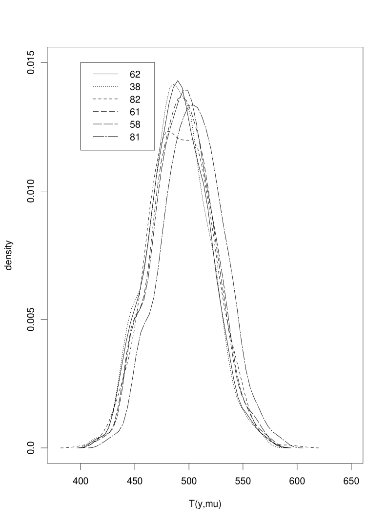
Figure 4: Kernel density estimate for the posterior distribution of $T^{(m)}(y,\mu)$.

7.2 Expected squared error loss

Figure 5: Model 38. Ratio of the posterior mean for the synthetic spectrum of model 38 to the observed spectrum of $\alpha$ Boo ($\rm{T}_{\rm eff}$ = 4230 K, $\log$ g = 1.50 dex, [Fe/H] = $-0.30$ dex) and posterior mean for the spectrum (full line) in band 1A.

Figure 6: Model 125. Ratio of the posterior mean for the synthetic spectrum of model 125 to the observed spectrum of $\alpha$ Boo ($\rm{T}_{\rm eff}$ = 4440 K, $\log$ g = 1.80 dex, [Fe/H] = 0.00 dex) and posterior mean for the spectrum (full line) in band 1A.

Model 38 ($\rm{T}_{\rm eff}$ = 4230 K, $\log g\,=\,1.50\,$ dex, [Fe/H] =  $-0.30$  dex) has the smallest value for $L_{38}^{2}$=$3.394\times 10^{6}$ while model 125 reaches the highest value, $L_{125}^{2}=5.7828\times 10^{6}$. Figs. 5 and 6 show the observed spectrum, the synthetic spectrum, and the posterior mean calculated from (13), for models 38 and 125. For model 38, the posterior mean and the observed spectrum closely agree along the entire wavelength range. The discrepancies are larger for model 125. Note how the posterior mean for the spectrum always lies between the observed and synthetic spectra. It is also clear for both models that the observed spectrum is more dominant at the end of band 1A. Especially for model 125 (Fig. 6), the posterior mean and the observed spectrum become closer when approaching the end of the band. Based on this model selection criterion, model 38 with stellar parameters $\rm{T}_{\rm eff}$ = 4230 K, $\log$ g = 1.50 dex and [Fe/H] = $-0.30$ dex is selected as providing the best representation of the band 1A ISO-SWS data of $\alpha$ Boo.

7.3 Determination of confidence intervals

Figure 7: Variance functions. The models were fitted by applying a linear mixed model for the data. Panel a: $\log$(STDEV-tag)² in band 1A with the estimated model and $95$ % credible intervals. Panel b: $\log$(SPARE-tag)² in band 1A with the estimated model and 95 % credible intervals. Panel c: shrinkage factor in band 1A with the estimated model and $95$ % credible intervals.

Fig. 7 shows the posterior means and the $95\%$ credible intervals for $\log(\sigma^{2})$ and $\log(\sigma^{2}_{M})$, as well as the shrinkage factor determined by a linear mixed model. The variance function for both $\sigma$ and $\sigma_{M}$ is substituted into the hierarchical model.

As was explained in Sects. 3.2 and 5, we had to restrict calculation of the synthetic spectra to a well-defined grid, with spacing determined by the analysis of Decin et al. (2000). However, as we only have the $L^{2}_{m}$ values for the predefined grid points, the accuracy of the derived parameter range for $\rm{T}_{\rm eff}$, $\log$ g, and [Fe/H] is bounded by the grid spacing. To estimate the confidence intervals around the stellar parameters and to test the sensitivity of the stellar parameters to 2.38–2.60 $\mu$m IR data of $\alpha$ Boo, we have constrained the choice of the stellar model and its descriptive parameters by investigating the behaviour of interpolated stellar models. This kind of procedure was also followed by Griffin & Lynas-Gray (1999), who have simulated a non-linear analytic function to the interpolated model flux for the purpose of a (frequentist) least-square analysis.

We chose not to interpolate between the synthetic spectra in the grid, but rather to calculate the stratification of a theoretical atmosphere model of intermediate mass, gravity or effective temperature by interpolating between theoretical models in the existing grid, and then to compute the corresponding synthetic spectrum. One may argue that for the type of medium-resolution spectra we are dealing with the difference between the two approaches, i.e., interpolation between the synthetic spectra of the existing grid versus computation of new synthetic spectra from interpolated theoretical model structures of intermediate $\Omega$, will be negligible. However, our purpose is to develop a general tool which, for example, may also be used for observed high-resolution spectra. Additionally, since spectral lines behave very non-linearly due to saturation, blending, complex dependency on the (molecular) opacities for cool-star atmospheres,… interpolating between synthetic spectra should be avoided. For the purpose of the interpolation between the models, the quantities as $T$ (temperature), $\log$ P_e (electron pressure), $\log$ P_g (gas pressure), $\log$ a_rad (radiative acceleration), and $\log\kappa$ (extinction coefficient) were interpolated linearly on $\log$ g or [Fe/H] (see e.g.  Plez, 1992). To interpolate in $\rm{T}_{\rm eff}$, the temperature distribution ${\rm{T_{new}}}(\tau)$ was scaled as ${\rm{T_{new}}(\tau)=(T_{eff}^{new}/T_{eff}^{old})*T_{old}(\tau)}$, followed by a pressure integration to calculate the proper P_e, P_g,…To judge upon the accuracy, we have interpolated between $\rm{T}_{\rm eff}$ = 4230 K and 4370 K to obtain $\rm{T}_{\rm eff}$ = 4300 K, between $\log$ g = 1.35 and 1.65 to obtain $\log$ g = 1.50, and between [Fe/H] = $-0.30$ and $-0.70$ to obtain [Fe/H] = $-0.50$ and have compared the interpolated model structures (and resulting synthetic spectra) with the existing models (and spectra) from the grid. The largest difference occurs for the model with the interpolated metallicity ([Fe/H] = $-0.50$) augmenting to 5 % for P_g at the outermost layer of the atmosphere model. This however only yields a discrepancy between the original theoretical spectrum and the one calculated from this interpolated model of maximum 0.1 % for a resolution of $~{}1500$ (while for a high-resolution spectrum of $\Delta\lambda=0.5$ Å, this augments to 0.55 %), proving the accuracy of our interpolation. Subsequently, we performed a 1-dimensional interpolation for the parameter values $\Omega$ of the selected top 10 models. The parameter spacing for the interpolated grid was $\Delta{\rm{T_{eff}}}$ = 5 K, $\Delta log$ g = 0.01 dex, and $\Delta$[Fe/H] = 0.01 dex. Synthetic spectra for these interpolated $\Omega$ were then computed.

Two comments are in place. First, the reduction of the number of models to the best 10 is not an intrinsic feature of the Bayesian method. Rather, having conducted the aforementioned frequentist analyses, such knowledge can be incorporated into the Bayesian analysis by way of expert priors. In addition, the choice for interpolation is not intrinsically linked to the Bayesian method neither, but rather should be viewed as one of the building blocks of our proposed method.

Confidence intervals for each of the three parameters were obtained by calculating the profile posterior likelihood for each of the interpolated models, by holding the two parameters fixed and using the interpolated grid over the third parameter. In total, 27 interpolated models for $\rm{T}_{\rm eff}$, 29 interpolated models for $\log$ g, and 39 interpolated models for [Fe/H] are constructed around one model. Let, for example, $G_{k}$, $k=1,\dots,27$, be the profile log-likelihood in temperature for the $k$th interpolated model. $G_{k}$ is conditioned upon the values of $\log$ g and [Fe/H]. The normalized profile log-likelihood is given by

$$R_{k}=\frac{G_{k}-\min(G_{k})}{\max(G_{k})-\min(G_{k})}.$$

The interval estimate for $\rm{T}_{\rm eff}$, $\log$ g or [Fe/H] is the set of all values of $\rm{T}_{\rm eff}$, $\log$ g or [Fe/H] for which the normalized profile likelihood exceeds 0.9. Table 4 and Fig. 8 exhibit a typical example for determining the confidence intervals (here, for model 62, having rank 1 when considering all evidence combined, both provided here and assembled from the literature). For all of the top 10 models, the range in the 90 % confidence intervals is $\sim 50$ K in temperature, $\sim 0.1$ dex in $\log$ g and $\sim 0.2$ dex in [Fe/H]. These values thus specify the precision by which the stellar parameters can be determined, including all sources of variability. As a consequence, the best set of stellar parameters with the associated model-dependent internal error estimates for $\alpha$ Boo consists of $\rm{T}_{\rm eff}$ = 4230 $\pm$ 25 K, $\log$ g = 1.50 $\pm$ 0.05 dex, and [Fe/H] = $-0.30\pm 0.10$ dex.

Our estimates assume that the model from which they are calculated is the correct one. Importantly though, this model itself is subject to uncertainty, illustrated by the fact that not a single model but, say, 10 models (Table 3) are reasonable candidates. Constructing ranges from such a collection of models is useful in its own right, but the information contained therein should ideally be translated into an additional variance term, to be added to the internal standard errors. This can formally be done by considering the total variability surrounding a parameter estimate $\hat{\beta}$:

$$\mbox{Var}(\hat{\beta})=E[\mbox{Var}(\hat{\beta})|{\cal M}]+\mbox{Var}[E(\hat{\beta})|{\cal M}],$$

where ${\cal M}$ represents ‘model’. The first term on the right hand side is the internal variance estimate, and is consistently estimated by the method outlined above. The second term stands for the variability across models. When choosing, for example, the best 10 models as a representative set, one merely needs to calculate the sample variance of the corresponding 10 estimates. For $\rm{T}_{\rm eff}$, one obtains 6312.2, added to $25^{2}$, yielding 6937.2 and producing an improved standard error: $\rm{T}_{\rm eff}$ = 4230 $\pm$ 83 K. For the other two quantities, the corresponding improved error estimates are: $\log$ g = 1.50 $\pm$ 0.15 dex, and [Fe/H] = $-0.30\pm 0.21$ dex. These error estimates are larger than those obtained by Griffin & Lynas-Gray (1999), who ignored the between-model variability.

Table 4: Posterior maximum profile likelihood and interval estimates for $\rm{T}_{\rm eff}$, $\log$ g and [Fe/H] for model 62.

Parameter	Maximum	(90 % C.I.)
$\rm{T}_{\rm eff}$	4295	(4273; 4323)
$\log$ g	1.47	(1.415; 1.52)
${\rm[Fe/H]}$	$-0.57$	($-0.67$; $-0.48$)

Figure 8: Profile likelihood for model 62. Panel (a): profile likelihood for $\rm{T}_{\rm eff}$, panel (b): profile likelihood for $\log$ g, and panel (c): profile likelihood for [Fe/H].

8 Discussion

8.1 Comparison with other statistical methods

The proposed Bayesian method can compete with other methods used nowadays for the evaluation of stellar spectra for deducing stellar parameters. To see this, we discuss in this section historical work in the same field and analyse sources of involved errors.

It would indeed be most convincing when we could compare our proposed Bayesian analysis with other (Bayesian) methods including both systematic and statistical observational error estimates consistently throughout the whole analysis of evaluating observational spectra with theoretical predicitons. However, as far as we are aware of, it is the first time that a statistical method including these specifications has been developed and used. Nowadays, state-of-the-art Bayesian computational techniques are more and more leaping into the astronomical field, however with the main purpose to detect a line in a spectral model or a source above background (Protassov et al., 2002, and references therein), to automatically classify stellar spectra (Cheeseman & Stutz, 1996), to analyze Poisson count data (Kraft et al., 1991), to analyze event arrival times of periodicity (Gregory & Loredo, 1992), to analyze helioseismology data (Morrow & Brown, 1988), to deconvolve astrophysical images (Gull, 1989). van Dyk et al. (1999) were the only ones who have employed Bayesian techniques to analyse low-count, high-resolution astrophysical spectral data. They however have modelled the source energy spectrum as a mixture of several Gaussian line profiles and a generalized linear model which accounts for the continuum, i.e., one assumes that a transformation (e.g., $\log$) of the model is linear in a set of independent variables, and they have not computed a full theoretical atmosphere model and corresponding synthetic spectrum.

The frequentist approach is the method most often used by astronomers. The basic approach for modelling data in both the Bayesian and the frequentist case is the same, the main difference being that a frequentist route often is more elaborate than its Bayesian counterpart: (i) one chooses or designs a figure-of-merit function yielding at the end best-fit parameters, (ii) one assesses the appropriateness of the estimated parameters from a goodness-of-fit analysis, and (iii) one finally tries to determine the likely errors, in an ad hoc fashion, for the best-fitting parameters. A few comments are in place: (1) many practitioners never proceed beyond item (i), (2) there are numerous instances of inappropriate use of frequentist methods since practitioners may fail to account for a method’s statistical limitations, calling substantive scientific results into question (as nicely illustrated by Protassov et al., 2002), and (3) many statistical methods, Bayesian and frequentist alike, are designed for use with closed-form expression. A few examples using this kind of frequentist approach include Katz et al. (1998); Griffin & Lynas-Gray (1999); Cami et al. (2000); de Bruyne et al. (2003); Decin et al. (2004). A nice example in which a linear regression method has been developed for the analysis of astronomical data with measurement errors and intrinsic scatter can be found in Akritas & Bershady (1996). As stated before, two important conditions made us shift away from frequentist methods: (1) the inclusion of both statistical and systematic measurement uncertainties, and (2) the non-availability of a closed analytic formula to represent the stellar spectrum.

8.2 On the application to the case-study of $\alpha$ Boo

Table 5 summarizes a comprehensive literature study on the estimated stellar parameters of our case-study $\alpha$ Boo. A more elaborate version of this table, listing additionally other parameters such as the luminosity, the mass, the ¹²C/¹³C-ratio, and a short description of the methods and/or data used by the various authors, can be found in the appendix of Decin et al. (2000). The table has been updated with the results of Krtička & Štefl (1999), Decin et al. (2004), and this study, the only ones using spectrum fitting to determine the stellar parameters for $\alpha$ Boo, during the past seven years. Provided that error estimates are given by the authors, they are listed in Table 5. It is clear that many authors do not provide estimates of precision. Second, those who do so typically do not distinguish between the sources of imprecision accounted for, with the noteworthy exception of Griffin & Lynas-Gray (1999) and Decin et al. (2004). These considerations underscore the usefulness of our method.

Table 5: Literature study of $\alpha$ Boo: the columns tabulate the effective temperature in Kelvin, the logaritm of the gravity in cm/s², and the metallicity, respectively. Values assumed or adopted are given in parenthesis. An error estimate is listed whenever provided by the authors.

Teff	$\log$ g	[Fe/H]	Reference
$4350\pm 50$	$1.95\pm 0.25$	$-0.5$	van Paradijs & Meurs (1974)
$4260\pm 50$	$0.90\pm 0.35$		Mäckle et al. (1975)
$4410\pm 80$			Blackwell & Shallis (1977)
4240			Linsky & Ayres (1978)
$4060\pm 150$			Scargle & Strecker (1979)
$4420\pm 150$			Blackwell et al. (1980)
(4260)	(1.6)		Lambert et al. (1980)
$4490\pm 100$	$2.01\pm 0.46$	$-0.56\pm 0.07$	Lambert & Ries (1981)
$4350\pm 435$			Manduca et al. (1981)
$4205\pm 150$			Tsuji (1981)
$4375\pm 50$	(1.5)	($-0.5$)	Frisk et al. (1982)
4350	1.8	($-0.51$)	Kjærgaard et al. (1982)
$4490\pm 200$	$2.6\pm 0.3$	$-0.55\pm 0.30$	Burnashev (1983)
4370			Burnashev (1983)
(4375)	(1.57)		Harris & Lambert (1984)
(4375)	$1.6\pm 0.2$	$-0.5$	Bell et al. (1985)
($4410$)	($>0.98$)	($-0.50$)	Gratton (1985)
($4225$)	$1.6\pm 0.2$	($-0.56$)	Judge (1986)
4400	1.7	$-0.6$	Kyröläinen et al. (1986)
(4375)	$1.5\pm 0.5$		Tsuji (1986)
($4300$)	(1.74)		Altas (1987)
$4294\pm 30$			di Benedetto & Rabbia (1987)
(4375)	$1.97\pm 0.20$	$-0.42$	Edvardsson (1988)
4321	(1.8)	($-0.51$)	Bell & Gustafsson (1989)
4340	1.9	$-0.39$	Brown et al. (1989)
$4294\pm 30$			Volk & Cohen (1989)
4300	2.0	$-0.69\pm 0.10$	Fernández-Villacañas et al. (1990)
$4280\pm 200$	$2.19\pm 0.27$	$-0.60\pm 0.14$	McWilliam (1990)
$4362\pm 45$			Blackwell et al. (1991)
$4250\pm 80$	$1.6\pm 0.3$		Judge & Stencel (1991)
($4375$)	$1.5\pm 0.5$		Tsuji (1991)
4265			Engelke (1992)
4450	$1.96-1.98$	$-0.5$	Bonnell & Bell (1993)
4350	$1.71-1.73$	$-0.5$	Bonnell & Bell (1993)
4250	$1.43-1.44$	$-0.5$	Bonnell & Bell (1993)
4250	$1.81-1.82$	$0.0$	Bonnell & Bell (1993)
$4300\pm 30$	$1.5\pm 0.2$	$-0.5\pm 0.1$	Peterson et al. (1993)
(4260)	(0.9)	($-0.77$)	Gadun (1994)
(4420)	(1.7)	($-0.50$)	Gadun (1994)
4362	2.4		Cohen et al. (1996)
$4303\pm 47$			Quirrenbach et al. (1996)
($4375$)	($1.5$)		Aoki & Tsuji (1997)
4300	1.4	$-0.47$	Pilachowski et al. (1997)
$4291\pm 48$			di Benedetto (1998)
4255			di Benedetto (1998)
$4628\pm 210$			Dyck et al. (1998)
4320			Hammersley et al. (1998)
$4321\pm 44$			Perrin et al. (1998)
		$-0.547\pm 0.021$	Taylor (1999)
$4290\pm 30$			Griffin & Lynas-Gray (1999)∗
$4291.9\pm 0.7$	$1.94\pm 0.05$	$-0.68\pm 0.02$	Griffin & Lynas-Gray (1999)∗∗
$4390\pm 90$	$2.0\pm 0.2$	$-0.27\pm 0.05$	Krtička & Štefl (1999)
$4320\pm 140$	$1.50\pm 0.15$	$-0.50\pm 0.20$	Decin et al. (2000)
4160 – 4300	1.35 – 1.65	$-0.30-0.00$	Decin et al. (2004)
$4230\pm 83$	$1.50\pm 0.15$	$-0.30\pm 0.21$	This paper

^∗: model-independent external errors; ^∗∗: model-dependent internal errors

Authors using spectroscopic requirements (i.e., ionisation balance, independence of the abundance of an ion versus the excitation potential and equivalent width) to estimate the stellar parameters for $\alpha$ Boo are van Paradijs & Meurs (1974), Mäckle et al. (1975), Lambert & Ries (1981), Bell et al. (1985), Edvardsson (1988), and Bonnell & Bell (1993). From these results, we infer that the values for $\rm{T}_{\rm eff}$ range between 4260 and 4490 K, for $\log$ g ranging between 0.90 and 2.01 dex, and for [Fe/H] ranging from $-0.56$ to $-0.60$ dex. The maximum quoted uncertainties are 100 K, 0.46 dex and 0.14 dex, respectively, although it is not always clear whether the authors mention an internal or external error estimate. As has been pointed out by, for example, Smith & Lambert (1985), one can easily assess an external error estimate by varying the derived parameter values. This normally results in $\Delta$$\rm{T}_{\rm eff}$ $\approx$ 200K, $\Delta\log$ g $\approx$ 0.2 dex and $\Delta$[Fe/H] $\approx$ 0.2 dex.

Only few authors used one or other form of spectrum fitting method to estimate stellar parameters, amongst them Scargle & Strecker (1979), Manduca et al. (1981), Peterson et al. (1993), Krtička & Štefl (1999), Decin et al. (2003), and Decin et al. (2004). In the first two of these manuscripts, the effective temperature was determined from the flux-curve shape alone, while in the others a part of the observational spectrum either in the visible or in the near-infrared was used. Values for $\rm{T}_{\rm eff}$ range between 4060 and 4390 K (with a maximum quoted uncertainty of 435 K from Manduca et al. (1981)), for $\log$ g between 1.5 and 2.0 dex (with maximum uncertainty 0.2 dex) and for [Fe/H] between $-0.27$ and $-0.50$ dex (with maximum uncertainty 0.1 dex). According to Krtička & Štefl (1999), the different estimates for the stellar parameters as determined from different spectral regions using a minimum least-square analysis range between 4200 and 4600 K for $\rm{T}_{\rm eff}$, between 1.53 and 2.35 for $\log$ g and between $-0.155$ and $-0.461$ for [Fe/H]. Peterson et al. (1993) tabulated as results: $\rm{T}_{\rm eff}$ = $4300\pm 30$ K, $\log$ g = $1.5\pm 0.2$ dex, and [Fe/H] = $-0.5\pm 0.1$ dex. We could however not trace back if the quoted error estimates include external errors or only internal uncertainties. Only Krtička & Štefl (1999); Decin et al. (2003); Decin et al. (2004) have applied a frequentist least-square method to optimize the stellar parameters for $\alpha$ Boo using spectrum fitting. None of them included systematic and statistical error estimates.

Including both error sources, $\sigma$ and $\sigma_{M}$ does not result in different ranges for the fundamental stellar parameters $\rm{T}_{\rm eff}$, $\log$ g and [Fe/H] of $\alpha$ Boo, relative to Decin et al. (2004), even though the latter authors did not take measurement errors into account. Possibly, the error measurements on the different data points are smaller than the difference between the observational data and even the best model, which then would not result in gain of evidence when including the errors. Comparing the ratio of the observational data to the synthetic data of model 62 (having rank 1) with $\sigma$ and $\sigma_{M}$, we note that all of them have the same order of magnitude. This also indicates that the remaining structure when considering $y(t)/\theta^{(62)}(t)$, as in Decin et al. (2004), is not due to measurement uncertainties but rather indicates that some pattern in the observational data is not captured by the theoretical predictions. Plausible explanations for this are: (1) the fact we kept the C (carbon), N (nitrogen), and O (oxygen) abundance and the microturbulence fixed, (2) problems with the temperature distribution in the outermost layers of the model photosphere leading to an underestimation of the low-level vibration-rotation lines of CO (carbon monoxide), and (3) problems with the data reduction.

9 Conclusions and future prospects

Estimating the stellar atmospheric parameters from an observed spectrum with given error estimates entails a model selection task in which we had to select a synthetic spectrum from a collection of 125 models. Frequentist methods based on the Kolmogorov-Smirnov test and $\chi^{2}$ statistics to assess the goodness-of-fit are unable to incorporate the so-called statistical and systematic measurement errors of the observational data into the analysis. Our hierarchical Bayesian model with a normal model for the likelihood and conjugate normal prior is capable of taking both of these errors into account. Using the Bayesian weighted $\chi^{2}$ statistics to assess the goodness-of-fit, the results based on the 2.38–2.60 $\mu$m ISO-SWS data of $\alpha$ Boo are as follows: $\rm{T}_{\rm eff}$ ranges between 4160 and 4440 K, $\log$ g ranges between 1.20 and 1.65 dex and [Fe/H] ranges between $-0.15$ and $-0.70$ dex. For the model selection process, we have used the predictive squared error loss function. The parameters of the model with the best representation of the ISO-SWS data are $\rm{T}_{\rm eff}$ = 4230 K $\pm 83$ K), $\log$ g = 1.50 dex $\pm 0.15$ dex), and [Fe/H] = $-$0.30 dex $\pm 0.21$ dex).

Not only here but for a range of applications it is convenient to first rank the synthetic spectra in the grid, without including $\sigma$ and $\sigma_{M}$. When including the observational errors, one then does not have to apply the Bayesian analysis to all models, like the 125 considered here, but only to a selection of models that are of interest, e.g., the models which have the highest ranks and perhaps a few other models which have a poor goodness-of-fit.

It would be of interest, though outside of the scope of this paper, to apply the proposed method to (1) a larger set of standard stellar candles analysed in Decin et al. (2003), (2) a 7-dimensional grid, in which not only the effective temperature, the gravity and the metallicity are variable, but also the carbon, nitrogen and oxygen abundance and the microturbulence, and (3) the synthesis analysis of high-resolution optical data.

We emphasize that the hierarchical Bayesian model as proposed in this paper is a general method which is able to objectively determine the parameter ranges using the synthesis technique. In contrast to previous studies, this Bayesian method incorporates the systematic and statistical measurement error in the analysis of the data, and so in the determination of the stellar parameters and their uncertainty intervals. A step-by-step algorithmic explanation of the Bayesian analysis developed in this paper and the source code thereof are available upon request.

References

- Akritas & Bershady (1996) Akritas M. G., Bershady M. A., 1996, Astrophys. J., 470, 706
- Altas (1987) Altas L., 1987, Astrophys. and Space Science, 134, 85
- Aoki & Tsuji (1997) Aoki W., Tsuji T., 1997, Astron. Astrophys., 328, 175
- Bell et al. (1985) Bell R. A., Edvardsson B., Gustafsson B., 1985, Mon. Not. Roy. Astron. Soc., 212, 497
- Bell & Gustafsson (1989) Bell R. A., Gustafsson B., 1989, Mon. Not. Roy. Astron. Soc., 236, 653
- Blackwell et al. (1991) Blackwell D. E., Lynas-Gray A. E., Petford A. D., 1991, Astron. Astrophys., 245, 567
- Blackwell et al. (1980) Blackwell D. E., Petford A. D., Shallis M. J., 1980, Astron. Astrophys., 82, 249