Exploring the Dark Energy Redshift Desert with the Sandage-Loeb Test

Abstract

We study the prospects for constraining dark energy at very high redshift with the Sandage-Loeb (SL) test – a measurement of the evolution of cosmic redshift obtained by taking quasar spectra at sufficiently separated epochs. This test is unique in its coverage of the “redshift desert”, corresponding roughly to redshifts between 2 and 5, where other dark energy probes are unable to provide useful information about the cosmic expansion history. Extremely large telescopes planned for construction in the near future, with ultra high resolution spectrographs (such as the proposed CODEX), will indeed be able to measure cosmic redshift variations of quasar Lyman-$\alpha$ absorption lines over a period as short as ten years. We find that these measurements can constrain non-standard and dynamical dark energy models with high significance and in a redshift range not accessible with future dark energy surveys. As the cosmic signal increases linearly with time, measurements made over several decades by a generation of patient cosmologists may provide definitive constraints on the expansion history in the era that follows the dark ages but precedes the time when standard candles and rulers come into existence.

I Introduction

Measurements of luminosity distance to Type Ia supernovae (SNe; SN ) in combination with the location of the acoustic peaks in the Cosmic Microwave Background (CMB) power spectrum CMBpeak , as well as the scale of the baryon acoustic oscillations (BAO) in the matter power spectrum SDSSbao provide an accurate determination of the geometry and matter/energy content of the universe. These measurements are almost exclusively sensitive to the cosmological parameters through a time integral of the Hubble parameter (or, the expansion rate). Although direct measurements of the Hubble parameter are feasible, they are typically difficult. For instance, the BAO probe radial modes are directly sensitive to $H(z)$ Hu_Haiman , but require exceedingly precise knowledge of individual galaxy redshifts. In addition, the few proposals to directly measure the expansion rate all propose to determine $H(z)$ at a few specific epochs: $z\lesssim 2$ (from, say, the BAO, or by measuring the relative ages of passively evolving galaxies Jimenez_Loeb ), $z\sim 1000$ (from the CMB Zahn_Zal ) and $z\sim 10^{9}$ (from the Big Bang Nucleosynthesis). In particular, a new cosmological window would open if we could directly measure the cosmic expansion within the “redshift desert”, ideally exploring $2\lesssim z\lesssim 5$.

During the early years of Big-Bang cosmology Allan Sandage studied a possibility of directly measuring the temporal variation of the redshift of extra-galactic sources Sandage . As explained in the next section, this temporal variation is directly related to the expansion rate at the source redshift. However, measurements performed at time intervals separated by less than $10^{7}$ years would have failed to detect the cosmic signal with the technology available at that time Sandage . In 1998 these ideas have been revisited by Loeb Loeb . He argued that spectroscopic techniques developed for detecting the reflex motion of stars induced by unseen orbiting planets could be used to detect the redshift variation of quasar (QSO) Lyman-$\alpha$ absorption lines. A sample of a few hundred QSOs observed with high resolution spectroscopy with a $\sim 10$ meter telescope could in fact detect the cosmological redshift variation at $\sim 1\sigma$ in a few decades. In what follows we will therefore refer to this method as the “Sandage-Loeb” (SL) test.

The astronomical community has since entertained increasingly ambitious ideas with proposals for building a new generation of extremely large telescopes ($30-100$ meter diameter) GMT ; TMT ; Euro50 ; ELT . Equipped with high resolution spectrographs, these powerful machines could provide spectacular advances in astrophysics and cosmology. The Cosmic Dynamics Experiment (CODEX) spectrograph has been recently proposed to achieve such a goal Pasquini ; Molaro .

The large number of absorption lines typical of the Lyman-$\alpha$ forest provide an ideal method for measuring the shift velocity. The latter can be detected by subtracting the spectral templates of a quasar taken at two different times. As quasar systems are now readily targeted and observable in the redshift range $2\lesssim z\lesssim 5$, we have a new test of the cosmic expansion history during the epoch just past the dark ages when the first objects in the universe are forming.

If dark energy is consistent to our simplest models — small zero-point energy of the vacuum or a slowly rolling scalar field — then it significantly speeds up the expansion rate of the universe at $z\lesssim 1$. Under the same assumption, dark energy is subdominant at redshift $z\gtrsim 1$, and almost completely negligible at $z\gtrsim 2$. One may therefore ask whether is worthwhile to probe $z\gtrsim 2$ anyway. The answer is affirmative: since we do not know much about the physical provenance of dark energy, it is useful to adopt an entirely empirical approach and look for the signatures of dark energy at all available epochs regardless of the expectations. This question has recently been studied in some detail by Linder Linder_darkages , who considered toy models of dark energy that have non-negligible energy density at high redshift.

In this paper we study the cosmological constraints that can be inferred from future observations of velocity shift and their impact on different classes of dark energy models. In Sec. II we review the physics behind the SL test, in Secs. III and IV we describe future constraints on standard and non-standard dark energy models respectively, and in Sec. V we discuss our results and future prospects.

II The Sandage-Loeb test

It is useful to firstly review a standard textbook calculation of the Friedmann-Robertson-Walker cosmology. Consider an isotropic source emitting at rest. Since it does not posses any peculiar motion, the comoving distance to an observer at the origin remains fixed. Then waves emitted during the time interval ($t_{\rm s}$, $t_{s}+\delta{t}_{\rm s}$) and detected later during ($t_{o}$, $t_{o}+\delta{t}_{o}$) satisfy the relation Sandage

$$\int_{t_{\rm s}}^{t_{o}}\frac{dt}{a(t)}=\int_{t_{\rm s}+\delta{t}_{\rm s}}^{t_{o}+\delta{t}_{o}}\frac{dt}{a(t)}.$$ (1)

where $t_{\rm s}$ is the time of emission and $t_{o}$ the time of observation. For small time intervals ($\delta{t}\ll t$) this gives the well known redshift relation of the radiation emitted by a source at $t_{\rm s}$ and observed at $t_{o}$,

$$1+z_{\rm s}(t_{o})=a(t_{o})/a(t_{\rm s}).$$ (2)

Let us now consider waves emitted after a period $\Delta{t}_{\rm s}$ at $t_{\rm s}+\Delta{t}_{\rm s}$ and detected later at $t_{o}+\Delta{t}_{o}$. Similarly to the previous derivation the observed redshift of the source at $t_{o}+\Delta{t}_{o}$ is

$$1+z_{\rm s}(t_{o}+\Delta{t}_{o})=a(t_{o}+\Delta{t}_{o})/a(t_{\rm s}+\Delta{t}_{\rm s}).$$ (3)

Therefore an observer taking measurements at times $t_{o}$ and $t_{o}+\Delta{t}_{o}$ would measure the following variation of the source redshift

$$\Delta{z}_{s}\equiv\frac{a(t_{o}+\Delta{t}_{o})}{a(t_{\rm s}+\Delta{t}_{\rm s})}-\frac{a(t_{o})}{a(t_{\rm s})}.$$ (4)

In the approximation $\Delta t/t\ll 1$, we can expand the ratio $a(t_{o}+\Delta t_{o})/a(t_{\rm s}+\Delta t_{\rm s})$ to linear order and further using the relation $\Delta{t}_{o}=[a(t_{o})/a(t_{\rm s})]\Delta{t}_{\rm s}$ (as it can be easily inferred from Eq. (1)) we obtain

$$\Delta z_{s}\approx\left[\frac{{\dot{a}}(t_{\rm o})-{\dot{a}}(t_{\rm s})}{a(t_{\rm s})}\right]\Delta{t}_{o}.$$ (5)

This redshift variation can be expressed as a spectroscopic velocity shift, $\Delta v\equiv c\Delta z_{s}/(1+z_{\rm s})$. Using the Friedmann equation to relate ${\dot{a}}$ to the matter and energy content of the Universe we finally obtain (see Loeb ):

$$\frac{\Delta{v}}{c}=H_{0}\Delta{t}_{0}\left[1-{E(z_{s})\over 1+z_{s}}\right],$$ (6)

where $H_{0}$ is Hubble constant, $E(z)\equiv H(z)/H_{0}$ is the (scaled) Hubble parameter at redshift $z$, $c$ is the speed of light, and we have normalized the scale factor to $a(t_{o})=1$ and neglected the contribution from relativistic components. For a constant dark energy equation of state we have

$$E(z)=\left[\Omega_{M}(1+z)^{3}+\Omega_{DE}(1+z)^{3(1+w)}+\Omega_{K}(1+z)^{2}\right]^{\frac{1}{2}}$$ (7)

where $\Omega_{M}$ and $\Omega_{DE}$ are the matter and dark energy density relative to critical, $\Omega_{K}=1-\Omega_{M}-\Omega_{DE}$ is the curvature, and $w$ is the dark energy equation of state.

Figure 1: Cosmic velocity shift as function of the source redshift in a flat universe for different values of $\Omega_{M}$ and $w$. A time interval of $10$ years has been assumed. The signal primarily depends on $\Omega_{M}$ and more weakly on $w$.

In Figure 1 we plot $\Delta v$ as function of the source redshift in the flat case for different values of $\Omega_{M}$ and $w$ assuming a time interval $\Delta t_{\rm o}=10$ years. As we can see $\Delta v$ is positive at small redshifts and becomes negative at $z\gtrsim 2$. Under the assumption of flatness the amplitude and slope of the signal depend mainly on $\Omega_{M}$, while the dependence on $w$ is weaker.

In spite of the tiny amplitude of the velocity shift, the absorption lines in the quasar Ly-$\alpha$ provide a powerful tool to detect such a small signal. As already pointed out in Loeb the width of these lines is of order $\sim 20$ ${\rm km/s}$, with metal lines even narrower. Although these are still a few orders of magnitude larger than the cosmic signal we seek to measure, each Ly-$\alpha$ spectrum has hundreds of lines. Therefore spectroscopic measurements with a resolution $R>20000$ for a sample of $\sim 100$ QSOs observed $\sim 10$ years apart can lead to a positive detection of the cosmic signal. Moreover astrophysical systematic effects such as peculiar velocities and accelerations can lead to negligible corrections Loeb . Local accelerations may indeed be more important, but due to their direction dependence they can be determined from velocity shift measurements of QSOs sampled in different directions on the sky.

In Pasquini the authors have performed Monte Carlo simulations of Lyman-$\alpha$ absorption lines to estimate the uncertainty on $\Delta v$ as measured by the CODEX spectrograph. The statistical error can be parametrized in terms of the spectral signal-to-noise $S/N$, the number of Ly-$\alpha$ quasar systems $N_{QSO}$, and the quasar’s redshift

$$\sigma_{\Delta v}=1.4\left(\frac{2350}{S/N}\right)\sqrt{\frac{30}{N_{QSO}}}\left(\frac{1+z_{QSO}}{5}\right)^{-1.8}{\rm\frac{cm}{s}},$$ (8)

(at $z<4$) where $S/N$ is defined per $0.0125A$ pixel. The source redshift dependence becomes flat at $z>4$. The numerical factor slightly changes with the source redshift, varying from $1.4$ at $z=4$ to $2$ at $z\approx 2$. This small variation arises because the number of observed absorption lines decreases with $z_{QSO}$. For simplicity we assume its value to be fixed to $1.4$. The large $S/N$ necessary to detect the cosmic signal implies that a positive detection is not feasible with current telescopes. However the CODEX spectrograph is currently being designed to be installed on the ESO Extremely Large Telescope; a $\sim 50$ meter giant that can reach the necessary signal-to-noise with just few hours integration.

In the next sections we describe the cosmological window that such observations could open, with particular focus on dark energy models.

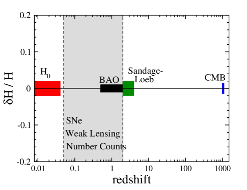
Figure 2: Fractional accuracy in the measurement of the Hubble parameter $H(z)$ as a function of redshift for a sample of cosmological probes. The accuracy and redshift ranges shown are best-guess values for the future surveys, and assume a single measurement of the Hubble parameter for each probe. Since SNe, number counts of clusters, and weak gravitational lensing do not measure the Hubble constant directly, but rather some combination of distances and (in the case of the latter two) growth of density perturbations, we only indicate their redshift range with the shaded region. The Sandage-Loeb overall constraint assumes roughly a 30 year survey and other specifications as in the text.

III Cosmological Parameters and Standard Dark Energy Models

We forecast constraints on cosmological parameters from velocity shift measurements using the Fisher matrix method for a LCDM fiducial cosmology. We assume experimental configuration and uncertainties similar to those expected from CODEX Pasquini ; Molaro . Namely we consider a survey observing a total of $240$ QSOs uniformly distributed in $6$ equally spaced redshift bins in the range $2\lesssim z\lesssim 5$, with a signal-to-noise $S/N=3000$, and the expected uncertainty as given by Eq. (8). Since there is no time integration involved in the computation of $\Delta v$ the Fisher matrix components can be easily determined analytically.

In Figure 2 we show the near-future status of measurements of the Hubble parameter at different cosmological epochs. We assume upcoming measurements of $H_{0}$ accurate to 2%, the overall BAO measurements of the expansion rate to 1% DETF , the CMB measurement of 1.4% Zahn_Zal , and the SL test measurement of $H$ using the assumptions outlined above. For clarity we do not show the Big Bang Nucleosynthesis constraint on $H(z)$ with $z=z_{\rm bbn}\approx 10^{9}$, which is accurate to $\sim 10$% (e.g. Copi ) and will improve as soon as the baryon density and deuterium abundance are more accurately determined. Since Type Ia supernovae, number counts of clusters, and weak gravitational lensing do not measure the Hubble constant directly, we only indicate their approximate redshift range with the shaded region. Clearly, the SL test is probing an era not covered with any other reliable cosmological probe.

In Figure 3 we plot the $1\sigma$ contours in the $\Omega_{M}-w$ plane as expected from type Ia supernovae, weak lensing power spectrum, power spectrum plus the bispectrum, and constraints expected from Planck’s measurement of distance to the last scattering surface. Supernova and weak lensing estimates are based on the SNAP mission SNAP , and SNe include systematic errors. The SL contour are complementary to those of other tests since $\Delta v$ probes a different degeneracy line in the $\Omega_{M}-w$ plane. It is worth noticing that such measurements are mostly sensitive to the matter density, as expected from the plot shown in Fig. 1. Allowing also for variation of the curvature, $\Omega_{\rm K}$, we find that the SL test alone determines the matter density about four times better than the curvature. As an example, for the 30-year survey the marginalized errors are $\sigma(\Omega_{M})=0.03$ and $\sigma(\Omega_{\rm K})=0.13$.

We have also found that limited accuracy in the Hubble constant measurement does not degrade the power of the SL test. For example, if $h$ is known to 0.04 (or to about 5%), the accuracy in $w$ is degraded by only 2% relative to the case when $h$ is perfectly known.

As far as dark energy is concerned, assuming a Gaussian prior on $h$ with $\sigma_{h}=0.04$, we obtain $\sigma_{w}=0.8$ for $\Delta{t}_{0}=10$ years time interval and $0.3$ for $30$ years. Thus the constraints on $w$ are not competitive with those inferred from other, well-established tests such as SNe Ia, weak lensing or BAO once we take into account that the latter probes will provide strong constraints by the time the SL test is undertaken. However, one should note that the constraints obtained by SL decrease linearly with time. For measurements made over a century, and with the expectedly larger number of QSOs, the SL limits on $w$ can easily be at the few percent level.

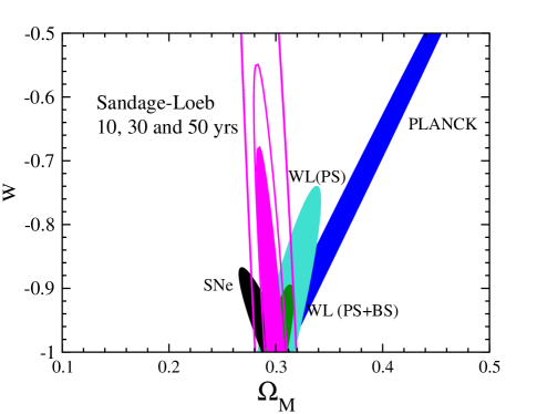
Figure 3: Constraints in the $\Omega_{M}-w$ plane for the SL test assuming (with increasingly smaller contours) a 10, 30 and 50-year survey and the number of quasars as in the text. We also show constraints expected from type Ia supernovae, weak lensing power spectrum, power spectrum in combination with bispectrum, and constraints expected from Planck’s measurement of distance to the last scattering surface. SNa and weak lensing estimates are based on the SNAP mission, and SNe also include systematic errors. The SL test contour is complementary to other constraints, and is mostly sensitive to the matter density, represented here by $\Omega_{M}$.

IV Non-standard dark energy models

A unique advantage of the SL test is that it probes the redshift range $2\lesssim z\lesssim 5$ which is very difficult to access otherwise. As mentioned in Section I, probing this redshift range is important for testing non-standard dark energy models that would otherwise be indistinguishable from those with a smooth, nearly or exactly constant equation of state function $w(z)$.

Figure 4: Cosmic velocity shift as function of the source redshift for a flat $\Lambda$CDM model with $\Omega_{m}=0.3$ (solid line), Chaplygin gas model (long dashed line) and an interactive dark energy-dark matter model (short dashed line) with $2\%$ deviation from standard redshift scaling of matter (see text). The error bars on the $\Lambda$CDM model assume a 10 year survey and other specifications as in the text.

WMAP observations in combination with low-redshift limits from SNe Ia impose a weak upper bound on the amount of dark energy deep during matter domination to be $\Omega_{DE}(z)<0.1$ Caldwell03 ; Corasaniti04 . Let us suppose that dark energy re-emerged at $3<z<5$ with $\Omega_{\rm DE}(z)=0.1$ in this range, while essentially zero at larger redshifts and that it behaved as a standard $\Lambda$CDM at $z<3$ (i.e. assuming standard $\Omega_{\rm DE}=0.75$, $w=-1$ values). We would like to distinguish such a model from a pure $\Lambda$CDM with $\Omega_{\rm DE}$ and $w$ as above. Clearly, low-redshift probes (SNe, BAO, galaxy clustering) cannot distinguish these two models since the required redshift is too high even for the most ambitious surveys. Furthermore, the distance to the last scattering surface between the two models differs only by 0.5%, which is too low to be observable even with Planck, since the 1-$\sigma$ uncertainty is about 0.4% with temperature and polarization information EisHuTeg . However, the two models can be distinguished via the SL test at about 3-$\sigma$ level, assuming only a 10-year survey and other specifications as in the previous section.

While the aforementioned scenario with dark energy emerging in the specific window at $3\lesssim z\lesssim 5$ may seem contrived, it is easy to find physically motivated models whose identification can significantly benefit from data in this “desert”. One example is given by scalar field models which predict the periodic emergence of DE at various epochs during the history of the universe oscillating ; Griest . Even though for these particular models one has to go to a much higher redshift to see the next phase where $\Omega_{\rm DE}=O(1)$, it is plausible, and certainly currently observationally allowed (e.g. flowroll ) that such a phase could have occurred somewhere within $2\lesssim z\lesssim 5$.

Another example is given by models with dark energy-dark matter interaction (see e.g. Damour ; Amendola ; Chimento ; KhouryWelt ; Peebles ; Das ; Alimi ). In the simplest realization where the scalar field only couples to dark matter, it mediates a long range interaction which causes two separate effects. First, dark matter particles, unlike the baryons, experience a scalar-tensor type of gravity, which modifies the Newtonian regime (see AmendolaPert ). The time and scale of when such type of modification becomes cosmologically relevant depend on the particular model considered. Second, dark matter particles acquire a time dependent mass whose evolution is determined by the specifics of the scalar field dynamics. As a consequence of this, the redshift evolution of the dark matter density deviates from the usual $(1+z)^{3}$. At low redshift, when the universe is dark energy dominated, these models cannot be distinguished from the standard $\Lambda$CDM . Therefore, the best way to probe models with such dark matter-dark energy interaction is to map out cosmic expansion during the matter dominated phase (see Figure 4). The SL tests offers a unique tool to do just that.

In order to forecast how well a deviation of the dark matter density from the $(1+z)^{3}$ law can be detected, we parametrize its redshift evolution as $\propto(1+z)^{3(1-b)}$ in the range $2\lesssim z\lesssim 5$, where $|b|<1$ is a constant free parameter. The scalar field, on the other hand, can be treated as a dark energy component with $w\approx-1$, since the field slowly rolls toward the minimum of its effective potential at late times Das . Assuming a flat fiducial model with $\Omega_{M}=0.3$ and $w=-1$, we find that the SL test can detect deviations from the standard matter scaling as small as $1\%$ (i.e. $b=0.01$) over $10$ years and $0.3\%$ for $30$ years. Therefore, SL test can provide constraints an order of magnitude tighter than those inferred using future SNe Ia or the Alcock-Paczynsky test Dalal . Since the deviation $b$ is generally a function of redshift, one can use the velocity shift measurements to reconstruct the redshift dependence of $b$, and then determine the strength and functional form of the scalar interaction.

The Chaplygin gas is yet another dark energy candidate that can be tested in the range of redshift probed by the SL test. Proposed as a phenomenological prototype of unified dark energy and dark matter model kam ; bil ; ben , it describes an exotic fluid with an inverse power law homogeneous equation of state, $P=-|w_{0}|\Omega_{\rm Ch}^{0}\rho_{0}/\rho^{\alpha}$ (e.g. Bean_Dore ), where $w_{0}$ is the present equation of state, $\Omega_{\rm Ch}^{0}$ is the current energy density of the gas $\rho_{0}=3H_{0}^{2}$ is the total energy density and $\alpha>-1$ is a dimensionless parameter. This corresponds to a fluid which behaves as dust in the past and as cosmological constant in the future. For $\alpha=0$ the model reduces to $\Lambda$CDM ave03 . The Chaplygin gas energy density evolves with redshift according to:

$$\Omega_{\rm Ch}(z)=\Omega_{\rm Ch}^{0}\left[-w_{0}+(1+w_{0})(1+z)^{3(\alpha+1)}\right]^{1\over 1+\alpha}.$$ (9)

As shown in Amendolafin this model can provide a good fit to current cosmological observables with $\Omega_{\rm Ch}\sim 0.95$ (with a baryonic component of $\Omega_{b}=0.05$), $w_{0}\sim-0.75$ and $\alpha=0.2$. From Fig. 4 we can see that although this model has a velocity shift at $z<1$ similar to that of a $\Lambda$CDM , it can be tested with high redshift measurements. For instance we find that, for this particular model, the Chaplygin parameters can be determined with uncertainties $\sigma_{w_{0}}=0.03$ and $\sigma_{\alpha}=0.04$ respectively and thus distinguished from the $\Lambda$CDM values at a high confidence level.

V Discussion

In this paper we have analyzed the prospects for constraining dark energy at high redshift ($2\lesssim z\lesssim 5$) by direct measurements of the temporal shift of the quasar Lyman-$\alpha$ absorption lines (the Sandage-Loeb effect). While the signal is extremely small, the physics is straightforward, and the measurement is certainly within reach of future large telescopes with high resolution spectrographs.

As the SL test mostly probes the matter density at high redshift, the constraints on standard dark energy models with a nearly or exactly constant equation of state $w$ are weaker than those that observations of SN Ia, BAO, weak lensing and number counts will be able to achieve in the future (although the SL test becomes competitive for measurements spread over a period of several decades or more). This is mostly because the sensitivity of cosmological probes to standard dark energy models is exhausted at $z\lesssim 2$ and higher redshift data do not improve them significantly (e.g. frieman ). However, the principal power of SL measurements at $2\lesssim z\lesssim 5$ comes from their ability to constrain non-standard dark energy models, where the dark energy density is non-negligible at higher redshifts — or equivalently, models where the total energy density does not scale with redshift as $(1+z)^{3}$ at $z\gtrsim 2$. In particular, as discussed in the previous section, in only one decade the SL measurements will allow to test the redshift scaling of the matter density with an accuracy one order of magnitude greater than standard cosmological tests.

Tighter constraints on standard dark energy models could be obtained if observations of Ly-$\alpha$ systems were feasible at $z\lesssim 2$. What are the prospects for performing the SL test at lower redshift? For this to be possible UV space-based instruments are necessary. Space-based UV Lyman-$\alpha$ astronomy is possible and has already produced remarkable results (see e.g penton04 ), though it generally lacks the spectral resolution and wavelength coverage of the higher redshift studies. However during the past few years high quality observations of several low redshift QSOs have been obtained with the Hubble Space Telescope (HST) and its Space Telescope Imaging Spectrograph (STIS). It is therefore conceivable that future space based experiments will be able to measure the SL effect at low redshift.

Other astrophysical probes that can potentially explore the redshift desert are not yet well understood. For instance, it might be possible to measure the angular diameter distance at redshift of 10-20 from the acoustic oscillations in the power-spectrum of the 21cm brightness fluctuations Barkana_Loeb . Further, gamma ray bursts (GRBs) (e.g. GRB ) have been proposed as alternative standard candles. These can probe roughly the same redshift range as the SL ($z\lesssim 6$). Similarly gravitational wave “standard sirens” can measure distances to GW sources all the way out to $z\sim 20$ Holz_Hughes . However, the prospects of turning the GRBs into standard candles is extremely uncertain at this time, and it is not clear that they can be used as cosmological probes. The GW sirens, while potentially providing amazingly accurate distance measurement, suffer from gravitational lensing of the signal, which adds an effective noise term to distance measurements and greatly degrades their power to constrain cosmological models Holz_Hughes . Conversely, the SL test is based on extremely simple physics and involves controllable systematic errors, but it does require a powerful instrument and patience to wait at least a decade before repeating the measurements in order to produce interesting results.

We finally point out that the velocity shift signal increases linearly with time, thus amply rewarding increased temporal separation between measurements. Therefore observations made over a period of several decades by a generation of patient cosmologists may provide definitive constraints on the expansion history in the era before the usual standard candles and rulers, Type Ia supernovae and acoustic oscillations in the distribution of galaxies, become readily available.

References

- (1) A. Riess et al., Astroph. J. 607, 665 (2004); P. Astier et al., Astron. & Astroph. 447, 31 (2006).
- (2) P. De Bernardis et al., Nature 404, 995 (2000); D. N. Spergel et al., Astroph. J. Supp. 148, 175 (2004).
- (3) D. J. Eisenstein et al., Astrophys. J. 633, 560 (2005).
- (4) W. Hu and Z. Haiman, Phys. Rev. D 68, 063004 (2003).
- (5) R. Jimenez and A. Loeb, Astrophys. J. 573, 37 (2002).
- (6) O. Zahn and M. Zaldarriaga, Phys. Rev. D 67, 063002 (2003)
- (7) A. Sandage, Astrophys. J. 139, 319 (1962).
- (8) A. Loeb, Astrophys. J. 499, L111 (1998), [astro-ph/9802122].
- (9) Giant Magellan Telescope; http://www.gmto.org/
- (10) Thirty Meter Telescope; http://www.tmt.org/
- (11) Euro50; http://www.astro.lu.se/%7Etorben/euro50/
- (12) European Extremely Large Telescope press release; http://www.eso.org/outreach/press-rel/pr-2006/pr-46-06.html
- (13) L. Pasquini et al., Proc. Int. Astron. Union 1, 193 (2005).
- (14) P. Molaro, M. T. Murphy and S. A. Levshakov, Proc. Int. Astron. Union 1, 198 (2005), [astro-ph/0601264].
- (15) E.V. Linder, Astropart. Phys. 26, 16 (2006) [astro-ph/0603584].
- (16) A. Albrecht et al, Dark Energy Task Force Report [astro-ph/0609591].
- (17) C. Copi, A. Davis and L.M. Krauss, Phys. Rev. Lett. 92, 171301 (2004)
-
(18)
SNAP – http://snap.lbl.gov ;
G. Aldering et al. 2004, astro-ph/0405232 - (19) R. R. Caldwell and M. Doran, Phys. Rev. D 69, 103517 (2004), [astro-ph/0305334].
- (20) P.S. Corasaniti, M. Kunz, D. Parkinson, B. A. Bassett and E. J. Copeland, Phys. Rev. D 70, 083006 (2004), [astro-ph/0406608].
- (21) D. Eisenstein, W. Hu, and M. Tegmark, Astrophys. J. 518, 2 (1999), [astro-ph/9807130];
- (22) S. Dodelson, M. Kaplinghat, and E. Stewart, Phys. Rev. Lett. 85, 5276 (2000).
- (23) K. Griest, Phys. Rev. D, 66, 123501 (2002), [astro-ph/0202052]
- (24) D. Huterer and H. Peiris, astro-ph/0610427
- (25) T. Damour, G.W. Gibbons and C. Gundlach, Phys. Rev. Lett. 64, 123 (190).
- (26) L. Amendola, Phys. Rev. D, 62, 043511 (2000); L. Amendola and D. Valentini, Phys. Rev. D, 64, 043509 (2001).
- (27) L. P. Chimento, A. S. Jakubi, D. Pavon and W. Zimdahl, Phys. Rev. 67, 083513 (2003).
- (28) J. Khoury and A. Weltman, Phys. Rev. Lett. 93, (2004) 172204.
- (29) G. R. Farrar and P. J. E. Peebles, Astrophys. J. 604, 1 (2004).
- (30) S. Das, P.S. Corasaniti and J. Khoury, Phys. Rev. D, 73, 083509 (2006).
- (31) A. Fuzfa and J.-M. Alimi, Phys. Rev. Lett. 97, 061301 (2006); A. Fuzfa and J.-M. Alimi, in preparation.
- (32) L. Amendola, Phys. Rev. D, 69, 103524 (2004), [astro-ph/0311175].
- (33) N. Dalal, K. Abazajian, E. Jenkins and A. V. Manohar, Phys. Rev. Lett. 87, 141302 (2001).
- (34) A. Kamenshchik, U. Moschella & V. Pasquier, V., 2001, Phys. Lett. B 511, 265 (2001).
- (35) N. Bilić, G.B. Tupper & R.D. Viollier, Phys. Lett. B 535, 17 (2002).
- (36) M.C. Bento, O. Bertolami & A.A. Sen, Phys. Rev. D 66, 043507 (2002).
- (37) R. Bean and O. Doré, Phys. Rev. D, 68, 023515 (2003).
- (38) P.P. Avelino, L.M.G. Beça, J.P.M. de Carvalho & C.J.A.P. Martins, JCAP 09, 002 (2003).
- (39) L. Amendola, I. Waga, F. Finelli, JCAP 0511 (2005) 009.
- (40) J.A. Frieman, D. Huterer, E.V. Linder and M.S. Turner, Phys. Rev. D, 67, 083505 (2003).
- (41) S. V. Penton et a., Astrophys. J. Suppl. 152, 29 (2004)
- (42) R. Barkana and A. Loeb, MNRAS, 363, L36 (2005).
- (43) B. Schaefer, astro-ph/0612285
- (44) D. Holz and S. Hughes, Astrophys. J. 629, 15 (2005)