Inflation over the hill

Abstract

We calculate the power spectrum of curvature perturbations when the inflaton field is rolling over the top of a local maximum of a potential. We show that the evolution of the field can be decomposed into a late-time attractor, which is identified as the slow roll solution, plus a rapidly decaying non-slow roll solution, corresponding to the field rolling “up the hill” to the maximum of the potential. The exponentially decaying transient solution can map to an observationally relevant range of scales because the universe is also expanding exponentially. We consider the two branches separately and we find that they are related through a simple transformation of the slow roll parameter $\eta$ and they predict identical power spectra. We generalize this approach to the case where the inflaton field is described by both branches simultaneously and find that the mode equation can be solved exactly at all times. Even though the slow roll parameter $\eta$ is evolving rapidly during the transition from the transient solution to the late-time attractor solution, the resultant power spectrum is an exact power-law spectrum. Such solutions may be useful for model-building on the string landscape.

I Introduction

The inflationary paradigm Guth:1980zm is one of the basic constituents of the standard cosmological model. By postulating a short period of accelerated expansion of the very early universe, it provides a natural explanation for the origin of structure as well as the flatness and homogeneity of the observable universe. In the simplest models, inflation is driven by a single scalar field (inflaton) which evolves slowly along a nearly flat potential. The quantum fluctuations of the inflaton can then be translated into perturbations in the early universe which are observed as temperature fluctuations in the cosmic microwave background (CMB) radiation. These models predict an almost scale-invariant spectrum with negligible non-gaussianities for the primordial density perturbations.

Unfortunately, the equations of motion for the inflaton field can not be solved analytically in general and certain approximations must be made in order to obtain exact solutions. The most powerful approximation is the slow roll approximation Albrecht:1982wi ; Steinhardt:1984jj ; Linde:1981mu , which assumes that the kinetic energy of the inflaton field is suppressed by the expansion, and at higher order amounts to the introduction of an infinite hierarchy of parameters Liddle:1994dx . It is then possible not only to obtain analytic solutions of the equation of motion of the field, but also to express the power spectrum in terms of the slow roll parameters.

Even though the slow roll approximation is widely used in the literature, it is by no means the only successful description of inflation. It is well known that the slow roll approximation, while it initially describes the evolution of the field with great accuracy, breaks down near the end of inflation. Moreover, one can find solutions in cases where slow roll is strongly violated Garcia-Bellido:1996ke ; Stewart:1993bc ; Linde:2001ae ; Kinney:1997ne ; Easther:1995pc ; Kinney:2005vj . It is therefore interesting to investigate inflation in situations where, even though the slow roll approximation is not valid, the power spectrum of curvature perturbations agrees with observations.

The paper is structured as follows: Section II presents a review of the single field inflation formalism. In section III we discuss the generation of curvature perturbations in inflation and we find an exact expression for a specific class of models. In section IV we study the case of the inflaton field rolling over the top of a local maximum of a potential. We show that even though the slow roll parameter $\eta$ is evolving rapidly and the inflationary solutions are initially far from slow roll, the mode equation can be solved exactly and the generated perturbations are consistent with observations. We apply this exact solution to the case of non-slow roll evolution considered in Ref. Kinney:2005vj . Section V contains a summary and conclusions.

II The single-field inflation formalism

In this section we review the basic formalism of single field inflation. The background metric that will be used in this paper is the flat FRW metric

$$ds^{2}=dt^{2}-a^{2}(t)d\mathbf{x}^{2}=a^{2}(\tau)[d\tau^{2}-d\mathbf{x}^{2}],$$ (1)

where $\tau$ is the conformal time, defined in terms of the coordinate time $t$ as

$$d\tau=\frac{1}{a}dt.$$ (2)

In what follows, overdots correspond to derivatives with respect to the coordinate time $t$, and primes to derivatives with respect to the field $\phi$. Assuming that the field $\phi$ dominates the energy density of the universe, the Einstein field equations become

$$H^{2}=\left(\frac{\dot{a}}{a}\right)^{2} = \frac{8\pi}{3m_{\rm Pl}^{2}}\left[V(\phi)+\frac{1}{2}\dot{\phi}^{2}\right],$$

$$\frac{\ddot{a}}{a} = \frac{8\pi}{3m_{\rm Pl}^{2}}\left[V(\phi)-\dot{\phi}^{2}\right].$$ (3)

The evolution of the scale factor $a$ is then given by the general expression

$$a\propto e^{-N},$$ (4)

where $N$ is defined to be the number of e-folds

$$dN\equiv-Hdt.$$ (5)

According to the above sign convention, $N$ gives the number of e-folds before the end of inflation and increases as one goes backwards in time.

The equation of motion for a spatially homogeneous scalar field $\phi$ in a FRW background can be written

$$\ddot{\phi}+3H\dot{\phi}+V^{\prime}(\phi)=0.$$ (6)

In the case that $\ddot{\phi}$ is negligible, we recover the slow roll approximation

$$3H\dot{\phi}+V^{\prime}(\phi)\simeq 0,$$ (7)

with

$$H^{2}\simeq{8\pi\over 3m_{\rm Pl}^{2}}V\left(\phi\right).$$ (8)

If the field $\phi$ is monotonic in time, we can express the Hubble parameter $H$ in terms of $\phi$ instead of the coordinate time $t$. This is in general more convenient since $H$ is not constant but varies as the field evolves along the potential. The dynamics of single field inflation can then be described by the so-called Hamilton-Jacobi formalism Muslimov:1990be ; Salopek:1990jq ; Lidsey:1995np , given by the following equation

$$\left[H^{\prime}(\phi)\right]^{2}-\frac{12\pi}{m_{\rm Pl}^{2}}H^{2}(\phi)=-\frac{32\pi^{2}}{m_{\rm Pl}^{4}}V(\phi),$$ (9)

and

$$\dot{\phi}=-\frac{m_{\rm Pl}^{2}}{4\pi}H^{\prime}(\phi).$$ (10)

This system of two first order equations is equivalent to the second order equation of motion (6).

We can then define the following Hubble slow roll parameters as derivatives of $H$ with respect to the field $\phi$

$$\epsilon\equiv\frac{m_{\rm Pl}^{2}}{4\pi}\left(\frac{H^{\prime}(\phi)}{H(\phi)}\right)^{2}\simeq\frac{m_{\rm Pl}^{2}}{16\pi}\left(\frac{V^{\prime}(\phi)}{V(\phi)}\right)^{2},$$ (11)

$$\eta\equiv\frac{m_{\rm Pl}^{2}}{4\pi}\frac{H^{\prime\prime}(\phi)}{H(\phi)}\simeq\frac{m_{\rm Pl}^{2}}{8\pi}\left[\frac{V^{\prime\prime}(\phi)}{V(\phi)}-\frac{1}{2}\left(\frac{V^{\prime}(\phi)}{V(\phi)}\right)^{2}\right],$$ (12)

and

$$\xi^{2}\equiv\frac{m_{\rm Pl}^{4}}{16\pi^{2}}\frac{H^{\prime}(\phi)H^{\prime\prime\prime}(\phi)}{H^{2}(\phi)}.$$ (13)

The last terms in Eqs. (11) and (12) are true only in the context of slow roll, in which case $\epsilon$ and $\eta$ are functions of the derivatives of the potential. In order for slow roll to be valid, the slope and the curvature of the potential should satisfy $V^{\prime}(\phi)\ll V(\phi)$ and $V^{\prime\prime}(\phi)\ll V(\phi)$, or in terms of the slow roll parameters $\epsilon\ll 1$ and $|\eta|\ll 1$.

We next derive identities which will be useful in the following discussion. Using Eq. (10) it can be shown that

$$H^{\prime\prime}(\phi)=-\frac{4\pi}{m_{\rm Pl}^{2}}\frac{\ddot{\phi}}{\dot{\phi}}.$$ (14)

Substituting back into Eq. (12) we find that

$$\eta=3+\frac{V^{\prime}(\phi)}{H\dot{\phi}},$$ (15)

where Eq. (6) was used. It should be noted that even though the above expression contains the first derivative of the potential, it is exact.

The slow roll parameters $\epsilon$ and $\eta$ can also be expressed in terms of the field $\phi$ and the number of e-folds $N$. Substituting Eq. (10) into (11) we find that

$$\epsilon=\frac{4\pi}{m_{\rm Pl}^{2}}\left(\frac{\dot{\phi}}{H}\right)^{2}.$$ (16)

Also from Eq. (5) it is obvious that

$$\dot{\phi}=-H\frac{d\phi}{dN},$$ (17)

and we then have

$$\epsilon=\frac{4\pi}{m_{\rm Pl}^{2}}\left(\frac{d\phi}{dN}\right)^{2}.$$ (18)

We can similarly express $\eta$ as a function of $\phi$. Differentiating Eq. (18) with respect to $N$

$$\frac{d\epsilon}{d\phi}=\frac{8\pi}{m_{\rm Pl}^{2}}\frac{d^{2}\phi}{dN^{2}},$$ (19)

where Kinney:2002qn

$$\frac{d\epsilon}{d\phi}=\frac{4\sqrt{\pi}}{m_{\rm Pl}}\sqrt{\epsilon}(\eta-\epsilon).$$ (20)

Equating the above two expressions and substituting back into Eq. (18), we find that

$$\eta=\left(\frac{d^{2}\phi}{dN^{2}}\right)\left(\frac{d\phi}{dN}\right)^{-1}+\epsilon.$$ (21)

In the next section, we summarize the generation of curvature perturbations in inflation and we find an exact expression for the curvature power spectrum in the special case where $\epsilon$ is small and $\epsilon\ll|\eta|$=constant.

III Curvature perturbations in inflation

Inflation provides a natural explanation for the large-scale structure of the universe. During inflation, quantum fluctuations of the inflaton field are stretched to scales much larger than the horizon size, creating metric perturbations Mukhanov:1981xt ; Hawking:1982my ; Guth:1982ec ; Bardeen:1983qw . These perturbations are of two kinds: scalar or curvature perturbations, which are responsible for structure formation, and tensor perturbations (gravitational waves). In this paper we will only consider scalar perturbations, which can be described using the gauge-invariant variable $u$ Mukhanov:1990me

$$u=a\delta\phi-\frac{a\dot{\phi}}{H}\mathcal{R},$$ (22)

where $\mathcal{R}$ is the metric curvature perturbation. On comoving hypersurfaces ($\delta\phi=0$), the curvature perturbation $\mathcal{R}$ can be written

$$\mathcal{R}=\left|\frac{u}{z}\right|,$$ (23)

where $z$ is defined as

$$z=\frac{a\dot{\phi}}{H}.$$ (24)

We then define the power spectrum of $\mathcal{R}$ in terms of its two-point correlation function

$$P^{1/2}_{\mathcal{R}}(k)=\left[\frac{k^{3}}{2\pi^{2}}\langle\mathcal{R}^{2}\rangle\right]^{1/2}.$$ (25)

Using Eq. (23), we can express $P_{\mathcal{R}}(k)$ as

$$P^{1/2}_{\mathcal{R}}(k)=\sqrt{\frac{k^{3}}{2\pi^{2}}}\left|\frac{u_{k}}{z}\right|,$$ (26)

where the mode function $u_{k}$ satisfies the equation Mukhanov:1985rz ; Mukhanov:1988jd

$$\frac{d^{2}u_{k}}{d\tau^{2}}+\left(k^{2}-\frac{1}{z}\frac{d^{2}z}{d\tau^{2}}\right)u_{k}=0,$$ (27)

and

$$\frac{1}{z}\frac{d^{2}z}{d\tau^{2}}=2a^{2}H^{2}\left(1+\epsilon+\epsilon^{2}-\frac{3}{2}\eta+\frac{1}{2}\eta^{2}-2\epsilon\eta+\frac{1}{2}\xi^{2}\right).$$ (28)

It should be noted that even though Eq. (28) is written in terms of the slow roll parameters, it is an exact result. In order to calculate the power spectrum $P_{\mathcal{R}}(k)$, we need to solve Eq. (27) and evaluate the quantity $|u_{k}/z|$ for every mode with comoving wavenumber $k$. During inflation, these modes evolve from a quasi-Minkowskian state that can be represented at short wavelengths by the Bunch-Davies vacuum

$$u_{k}\propto e^{-ik\tau}\hskip 28.45274ptk\tau\rightarrow-\infty.$$ (29)

When the mode evolves to a wavelength much greater than the horizon size, the solution is

$$u_{k}\propto z\hskip 42.67912ptk\tau\rightarrow 0.$$ (30)

Equation (29) together with the canonical quantization condition for the fluctuations

$$u_{k}^{*}\frac{du_{k}}{d\tau}-u_{k}\frac{du_{k}^{*}}{d\tau}=-i,$$ (31)

completely specifies the initial conditions for the modes $u_{k}$.

Power-law inflation, for which $\epsilon=\eta=\xi=$ constant, is a case where Eq. (27) can be solved exactly, with a solution proportional to a Hankel function of the first kind:

$$u_{k}\propto\sqrt{-k\tau}H_{\nu}(-k\tau),$$ (32)

where

$$\nu=\frac{3}{2}+\frac{\epsilon}{1-\epsilon}.$$ (33)

For the slow roll approximation, assuming that the slow roll parameters $\epsilon$ and $\eta$ are small and approximately constant, the solution of the mode equation is again given by Eq. (32) with

$$\nu=\frac{3}{2}+2\epsilon-\eta.$$ (34)

Finally, the case of de Sitter expansion can be obtained from both the power law and the slow roll results, in the limit of $\epsilon\rightarrow 0$ and $\eta\rightarrow 0$.

We can equivalently express Eq. (27) in terms of the variable $y$, which is defined as

$$y=\frac{k}{aH},$$ (35)

and is the ratio of the wavelength of the mode relative to the horizon size. The variable $y$ is related to the conformal time $\tau$ by

$$dy=-k(1-\epsilon)d\tau,$$ (36)

and the mode equation (27) becomes

$$y^{2}(1-\epsilon)^{2}\frac{d^{2}u_{k}}{dy^{2}}+2y\epsilon(\epsilon-\eta)\frac{du_{k}}{dy}+\left[y^{2}-F(\epsilon,\eta,\xi)\right]u_{k}=0,$$ (37)

where

$$F(\epsilon,\eta,\xi)=2\left(1+\epsilon+\epsilon^{2}-\frac{3}{2}\eta+\frac{1}{2}\eta^{2}-2\epsilon\eta+\frac{1}{2}\xi^{2}\right).$$ (38)

A case of special interest in this paper is the one where the slow roll parameter $\epsilon$ is small and $\eta$ is approximately constant. The mode equation reduces then to

$$y^{2}\frac{d^{2}u_{k}}{dy^{2}}+\left[y^{2}-(2-3\eta+\eta^{2})\right]u_{k}=0,$$ (39)

with the following normalized solution,

$$u_{k}=\frac{1}{2}\sqrt{\frac{\pi}{k}}[\sqrt{y}H_{\nu}(y)],$$ (40)

where, for $\eta<3/2$,

$$\nu=3/2-\eta.$$ (41)

The power spectrum of curvature perturbations is evaluated in the long-wavelength limit,

$$P^{1/2}_{\mathcal{R}}(k)=\sqrt{\frac{k^{3}}{2\pi^{2}}}\left|\frac{u_{k}}{z}\right|_{y\rightarrow 0},$$ (42)

which is given in terms of the variable $y$ by

$$P^{1/2}_{\mathcal{R}}(k)=\mathcal{V}(\nu)\left(\frac{H^{2}}{2\pi\dot{\phi}}y^{3/2-\nu}\right),$$ (43)

with

$$\mathcal{V}(\nu)=2^{\nu-3/2}\frac{\Gamma{(\nu)}}{\Gamma{(3/2)}}.$$ (44)

The scalar spectral index $n$ is defined by differentiating Eq. (43) at constant time, or equivalently, constant scale factor:

$$n-1\equiv\left.\frac{d\ln P_{\mathcal{R}}}{d\ln k}\right|_{aH=const.}=3-2\nu=2\eta.$$ (45)

We emphasize that the definition of the curvature power spectrum in the long-wavelength limit Eq. (42), can differ substantially from the widely used definition of $P_{\mathcal{R}}$ as evaluated at horizon crossing

$$P^{1/2}_{\rm Hor}(k)=\sqrt{\frac{k^{3}}{2\pi^{2}}}\left|\frac{u_{k}}{z}\right|_{y=1}.$$ (46)

In the slow roll limit, Eqs. (42) and (46) are equivalent to second order in the slow roll parameters. However, in situations where slow roll is strongly violated, the horizon crossing expression for the power spectrum cannot be used, and care must be taken to correctly evaluate the power spectrum in the long-wavelength limit. (See Ref. Kinney:2005vj for a detailed discussion of the breakdown of the horizon crossing formalism far from slow roll.)

In the next section, we specialize to a particular case of non-slow roll evolution, which corresponds to a field rolling over the top of a local maximum of a potential.

IV Inflation over the hill

The specific example of non-slow roll evolution we consider here is a scalar field rolling over the top of a local maximum of a potential. This can be seen to be intrinsically non-slow roll, since in the slow roll limit

$$\dot{\phi}\propto V^{\prime}\left(\phi\right)=0,$$ (47)

at the maximum of the potential. The slow roll solution therefore automatically corresponds to a solution with the field stationary at the maximum of the potential in the infinite past. In a realistic situation, for example a field evolving in the string landscape, the field velocity may well be nonzero near the maximum. Since slow roll inflation is generically an attractor solution Liddle:1994dx , the evolution may still relax to the slow roll attractor at late times even if it is far from slow roll at early times.

We consider a potential of the form

$$V(\phi)=\Lambda^{4}\left[1-\frac{1}{2}\left(\frac{\phi}{\mu}\right)^{2}\right].$$ (48)

If the mass term of the inflaton is unsuppressed, the above expression will be a good approximation for any single-field potential as long as the inflaton is sufficiently close to the maximum. The equation of motion (6) can then be written as

$$\ddot{\phi}+3H\dot{\phi}-\frac{\Lambda^{4}}{\mu^{2}}\phi=0.$$ (49)

Assuming that $\dot{\phi}\ll V(\phi)$ and $\phi\ll\mu$, the Hubble parameter $H$ can be treated as approximately constant:

$$H\approx\sqrt{\frac{8\pi}{3m_{\rm Pl}^{2}}\Lambda^{4}}.$$ (50)

Following the standard slow roll approximation, the second order differential equation of motion (49) reduces to the first order Eq. (7), with $\dot{\phi}\propto V^{\prime}\left(\phi\right)$. But if one considers the full equation of motion (49), it can be shown Inoue:2001zt that the evolution of $\phi$ can be decomposed into a slowly varying branch, which is identified as the slow roll solution, plus a rapidly changing branch proportional to $a^{-3}(t)$. In this paper we relax the slow roll assumption and we study the full equation of motion of the field.

Equation (49) can be expressed in terms of the number of e-folds $N$ by using Eq. (5) as

$$\frac{d^{2}\phi}{dN^{2}}-3\frac{d\phi}{dN}-\alpha\phi=0,$$ (51)

where $\alpha$ is given by

$$\alpha=\frac{\Lambda^{4}}{\mu^{2}H^{2}}\approx\frac{3}{8\pi}\left(\frac{m_{\rm Pl}}{\mu}\right)^{2}.$$ (52)

The general solution of the equation of motion (51) is then

$$\phi(N)=\phi_{+}e^{r_{+}N}+\phi_{-}e^{r_{-}N},$$ (53)

with

$$r_{\pm}=\frac{3}{2}\left(1\mp\sqrt{1+\frac{4}{9}\alpha}\right).$$ (54)

If $\alpha$ is small, the square root can be expanded and the constants $r_{\pm}$ become

$$r_{+} = -\frac{\alpha}{3},$$

$$r_{-} = 3+\frac{\alpha}{3}.$$ (55)

The general solution (53) has two distinguishable branches: a transient branch $r_{-}$ which dominates at early time, and a “slow rolling” branch $r_{+}$ which can be identified as the late-time attractor. Since $\alpha$ is positive definite, $r_{\pm}$ will always be real, and an inflationary solution will exist for any set of chosen parameters $\Lambda^{4}$ and $\mu$.

In what follows, we assume that the solution (53) describes the evolution of the field for some range of inflation, and we look for new features when calculating the curvature power spectrum. From Eqs. (53) and (54) it is clear that the ratio of the transient branch over the “slow rolling” one decreases exponentially. That means that both branches will be equal at some value of the number of e-folds $N_{0}$. We can arbitrarily set $N_{0}$ by choosing the relative strength of the parameters $\phi_{+}$ and $\phi_{-}$ in Eq. (53). Despite the fact that the $r_{-}$ branch is exponentially decaying relative to the $r_{+}$ branch, the transient “fast roll” evolution can still correspond to an observationally relevant range of scales. This can easily be seen by considering the relation between the comoving wavenumber and the field value Liddle:1994cr :

$$d(\ln{k})=\frac{2\sqrt{\pi}}{m_{pl}}\frac{(\epsilon-1)}{\sqrt{\epsilon}}d\phi.$$ (56)

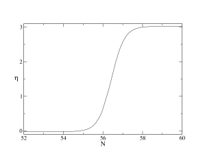
Even though the field displacement which corresponds to the transient branch is small, in the limit that $\epsilon$ is small, the field evolution during the transient can be mapped to a large range of comoving wavenumbers. This is also evident in the particular case shown in Fig. 1, where the transition between the transient and the attractor solution lasts about four e-folds of expansion.

In the following two subsections, we calculate the curvature power spectrum for two cases. We first consider each branch separately, for which $\eta$ is approximately constant. We then calculate the power spectrum in the region where the field evolves from the $r_{-}$ to the $r_{+}$ branch and $\eta$ is evolving rapidly.

IV.1 $\phi=\phi_{\pm}e^{r_{\pm}N}$

For simplicity, we first consider the two solutions in Eq. (53) separately. Using Eqs. (18) and (21), the slow roll parameters are given by

$$\epsilon = 4\pi r_{\pm}^{2}\left(\frac{\phi}{m_{\rm Pl}}\right)^{2},$$

$$\eta = r_{\pm}+\epsilon.$$ (57)

Near the maximum of the potential, $\phi\approx 0$ and $\epsilon\ll 1$, so that

$$\eta\approx r_{\pm}=constant.$$ (58)

Even though $\epsilon$ is assumed to be small, it is obvious from Eqs. (IV) and (58) that the $r_{-}$ branch will never satisfy the slow roll conditions, since $\eta>3$ always. For the $r_{+}$ branch, the slow roll limit is obtained for $\alpha\ll 1$ for which

$$|\eta_{SR}|\approx\frac{\alpha}{3}\ll 1.$$ (59)

This is the limit which will be of observational interest, since the late-time attractor corresponds to a nearly scale-invariant power spectrum consistent with observations.

The mode equation (37) for the curvature perturbations can then be written in either limit as

$$y^{2}\frac{d^{2}u_{k}}{dy^{2}}+[y^{2}-(2-3\eta+\eta^{2})]u_{k}=0,$$ (60)

where all the $\epsilon$ terms have been neglected. The above equation is invariant under the transformation $\eta\rightarrow 3-\eta$, and hence any pair $\eta_{1}$ and $\eta_{2}$ that satisfies

$$\eta_{2}=3-\eta_{1},$$ (61)

will give the same mode equation and therefore the same solution. It should be noted that the above invariance breaks down in the case of a non-negligible $\epsilon$. Since $\epsilon$ is negligible, $\dot{\phi}$ is small and therefore calling the transient solution “fast roll” is something of a misnomer, despite the fact that it is not slow roll.

The parameters $r_{\pm}$ defined in Eq. (IV), satisfy Eq. (61) and therefore lead to the same mode equation, which can be solved analytically. The solutions are proportional to a Hankel function of the first kind

$$u_{k}\propto\sqrt{y}H_{\nu}(y),$$ (62)

where

$$\nu=\left|\frac{3}{2}-\eta\right|.$$ (63)

The absolute value of $\nu$ is a consequence of the fact that the mode equation is the same for both branches. This means that the Hankel functions should be of the same order in both cases, and this requirement is satisfied by Eq. (63). The significance of the absolute value can also be seen by considering the general solution of the mode equation (60),

$$u_{k}=\frac{1}{2}\sqrt{\frac{\pi}{k}}\sqrt{y}[a_{k}H_{\nu}(y)+b_{k}H_{\nu}^{*}(y)].$$ (64)

When the mode is well inside the horizon, the above equation becomes

$$u_{k}\propto a_{k}e^{iy}+b_{k}e^{-iy}.$$ (65)

The Bunch-Davies vacuum is obtained by setting $b_{k}=0$ and $a_{k}=1$. If instead we look at the general solution for $\nu\rightarrow-\nu$, we can use the identity

$$H_{-\nu}=e^{i\nu\pi}H_{\nu},$$ (66)

to write

$$u_{k}=\frac{1}{2}\sqrt{\frac{\pi}{k}}\sqrt{y}[\tilde{a}_{k}H_{-\nu}(y)+\tilde{b}_{k}H_{-\nu}^{*}(y)]$$ (67)

$$=\frac{1}{2}\sqrt{\frac{\pi}{k}}\sqrt{y}[e^{i\nu\pi}\tilde{a}_{k}H_{\nu}(y)+e^{-i\nu\pi}\tilde{b}_{k}H_{\nu}^{*}(y)],$$ (68)

which corresponds to the Bunch-Davies boundary condition for $\tilde{a}_{k}=e^{-i\nu\pi}$ and $\tilde{b}_{k}=0$. Therefore $\nu\rightarrow-\nu$ introduces an irrelevant overall phase shift. This corresponds precisely to the symmetry of the mode equation (60) under the transformation $\eta\rightarrow 3-\eta$.

The power spectrum of curvature perturbations can be calculated from Eq. (43)

$$P_{\mathcal{R}}^{1/2}\propto k^{3/2}\left|u_{k}\over z\right|_{y\rightarrow 0}\propto\frac{H^{2}}{2\pi\dot{\phi}}y^{3/2-\nu},$$ (69)

and since $\nu$ takes the same value for both the $\eta=r_{+}$ and $\eta=r_{-}$ cases,

$$P_{\mathcal{R}}^{1/2}\propto\frac{H^{2}}{2\pi\dot{\phi}}y^{r_{+}},$$ (70)

for both branches. The scalar spectral index is then given by

$$n-1=\left.\frac{d\ln P_{\mathcal{R}}}{d\ln k}\right|_{aH={\rm const.}}=2r_{+},$$ (71)

which is the first order slow roll expression for the spectral index in the small $\epsilon$ limit for the slowly evolving $r_{+}$ branch. From Eq. (IV) it is clear that the choice $\alpha=0.075$ corresponds to

$$n=0.95,$$ (72)

which is within the region favored by the WMAP3 data Spergel:2006hy ; Alabidi:2006qa ; Seljak:2006bg ; Kinney:2006qm ; Martin:2006rs .

Even though therefore the field may evolve in a region where the slow roll approximation is strongly violated ($\eta\rightarrow 3^{+}$), the resultant power spectrum is identical to the one given by an evolution that satisfies the slow roll approximation ($\eta\rightarrow 0^{-}$) as a result of the invariance of the mode equation under the transformation given by Eq. (61). Note that the $\eta=3$ case corresponds to ultra slow roll inflation Tsamis:2003px , which gives an exact scale invariant spectrum. Evaluating the mode function at horizon crossing, results in an incorrect expression for the shape of the power spectrum Eq. (46), since

$$n_{\rm Hor}-1=\left.\frac{d\ln P_{\mathcal{R}}}{d\ln k}\right|_{k=aH}=2\eta=2r_{-}.$$ (73)

Finally, it can be shown that the transient $r_{-}$ branch describes a field rolling up an inverted potential. Re-expressing the derivative of the potential with respect to the field in Eq. (15), as a derivative with respect to the number of e-folds

$$\eta=3-\frac{1}{\dot{\phi}^{2}}\frac{dV(\phi)}{dN}.$$ (74)

For the $r_{-}$ branch, $\eta>3$, so that

$$\frac{dV(\phi)}{dN}<0,$$ (75)

and since $dN<0$ during inflation, we find that the field is rolling up the potential,

$$\Delta V(\phi)>0.$$ (76)

We next consider the transition from the transient solution to the late-time attractor.

IV.2 $\phi=\phi_{+}e^{r_{+}N}+\phi_{-}e^{r_{-}N}$

In the previous section we showed that the transient $r_{-}$ branch, even though it describes inflationary solutions far form slow roll, generates curvature perturbations that are consistent with observations as a result of the invariance of the mode equation under the transformation (61). These perturbations are identical to the ones produced by the $r_{+}$ branch, and in that sense the two branches are indistinguishable in terms of observables, since they both produce negligible gravitational waves. The $r_{-}$ branch, however, corresponds to the intrinsically non-slow roll solution of a field rolling up the hill of an inverted potential. In this section, we investigate the power spectrum produced during the transition from the transient $r_{-}$ branch to the late-time slow roll solution represented by the $r_{+}$ branch. During this transition, the parameter $\eta$ varies rapidly, and it is reasonable to expect a feature in the curvature power spectrum at scales corresponding to that transition. Remarkably, we find that no such feature exists.

In order for the field $\phi$ to be monotonic in time, $\dot{\phi}$ must not change sign. This requirement can be expressed in terms of $N$ as follows

$$\frac{d\phi}{dN}=r_{+}\phi_{+}e^{r_{+}N}+r_{-}\phi_{-}e^{r_{-}N}\neq 0,$$ (77)

assuming that the derivative of the field with respect to $N$ is a smooth function throughout its evolution. Since the signs of the constants $r_{\pm}$ are known from Eq. (54), the above condition can be achieved only if one of the coefficients $\phi_{\pm}$ is negative. We take $\phi_{-}<0$, which results in a positive time derivative for the field

$$\dot{\phi}=-H\frac{d\phi}{dN}>0.$$ (78)

Using Eqs. (18) and (21), the slow roll parameters are then given exactly by

$$\epsilon = \frac{4\pi}{m_{\rm Pl}^{2}}\left(r_{+}\phi_{+}e^{r_{+}N}+r_{-}\phi_{-}e^{r_{-}N}\right)^{2},$$

$$\eta = \frac{r_{+}^{2}\phi_{+}e^{r_{+}N}+r_{-}^{2}\phi_{-}e^{r_{-}N}}{r_{+}\phi_{+}e^{r_{+}N}+r_{-}\phi_{-}e^{r_{-}N}}+\epsilon,$$ (79)

where in the small $\epsilon$ limit

$$\eta\approx\frac{r_{+}^{2}\phi_{+}e^{r_{+}N}+r_{-}^{2}\phi_{-}e^{r_{-}N}}{r_{+}\phi_{+}e^{r_{+}N}+r_{-}\phi_{-}e^{r_{-}N}}.$$ (80)

According to the above sign convention for $\phi_{-}$, the denominator in Eq. (80) never crosses zero and $\eta$ is always finite. Equation (80) also reproduces both Eqs. (58) in the limiting case where one of the two branches vanishes.

Expressing the slow roll parameter $\xi^{2}$ in terms of $\epsilon$ and $\eta$ as Kinney:2002qn

$$\xi^{2}=\frac{d\eta}{dN}+\epsilon\eta,$$ (81)

and ignoring all the terms of order $\epsilon$, the mode equation becomes

$$y^{2}\frac{d^{2}u_{k}}{dy^{2}}+\left[y^{2}-F(\eta)\right]u_{k}=0,$$ (82)

where

$$F(\eta)=2-3\eta+\eta^{2}+\frac{d\eta}{dN}.$$ (83)

Equation (82) is no longer invariant under the transformation (61) since

$$F(\eta)\neq F(3-\eta).$$ (84)

Even though the mode equation does not respect the above symmetry, it can be solved analytically. In order to see that, we first note that both branches will be equal at some number of e-folds $N_{0}$

$$\phi_{+}e^{r_{+}N_{0}}=-\phi_{-}e^{r_{-}N_{0}}.$$ (85)

Equation (53) then becomes

$$\phi=A\left[e^{r_{+}(N-N_{0})}-e^{r_{-}(N-N_{0})}\right],$$ (86)

where

$$A=\phi_{+}e^{r_{+}N_{0}}=-\phi_{-}e^{r_{-}N_{0}}.$$ (87)

We are therefore able to absorb the coefficients $\phi_{\pm}$ into $A$ using the equality of the branches at $N=N_{0}$, and Eq. (80) takes then the simpler form

$$\eta=\frac{r_{+}^{2}e^{r_{+}(N-N_{0})}-r_{-}^{2}e^{r_{-}(N-N_{0})}}{r_{+}e^{r_{+}(N-N_{0})}-r_{-}e^{r_{-}(N-N_{0})}}.$$ (88)

Figure 1 shows $\eta$ as a function of $N$ for the case of $N_{0}=58$ and $\alpha=0.075$, where it can be seen that the transition from the $r_{-}$ to the $r_{+}$ branch lasts for approximately four e-folds.

Figure 1: $\eta$ as a function of $N$ for $N_{0}=58$ and $\alpha=0.075$

Using Eq. (88) it can also be shown that

$$\frac{d\eta}{dN}=-\frac{r_{+}r_{-}(r_{+}-r_{-})^{2}e^{(N-N_{0})(r_{+}+r_{-})}}{\left[r_{+}e^{r_{+}(N-N_{0})}-r_{-}e^{r_{-}(N-N_{0})}\right]^{2}}.$$ (89)

We therefore have analytic expressions for the slow roll parameter $\eta$ and its derivative. Substituting back these two equations into Eq. (83), we can find an exact expression for the function $F(\eta)$. After some straightforward but tedious algebra, and using the full expressions (54) for the parameters $r_{\pm}$ it can be shown that

$$F(\eta)=2+\alpha,$$ (90)

for any value of $N_{0}$. Even though $\eta$ evolves rapidly during the transition between the two branches (Fig. 1), the function $F(\eta)$ remains constant, and Eq. (82) becomes

$$y^{2}\frac{d^{2}u_{k}}{dy^{2}}+\left[y^{2}-(2+\alpha)\right]u_{k}=0.$$ (91)

This invariance of the $z^{\prime\prime}/z$ term in the mode equation is an example of the duality invariance considered by Wands in Ref. Wands:1998yp , and a non-slow roll solution exhibiting the same invariance was obtained by Leach and Liddle in Ref. Leach:2000yw for a different choice of potential. More recently, Starobinsky Starobinsky:2005ab has constructed a non-slow roll solution resulting in an exactly scale-invariant spectrum.

The solution of Eq. (91) can be written in terms of a Hankel function

$$u_{k}\propto\sqrt{y}H_{\nu}(y),$$ (92)

where

$$\nu=\frac{3}{2}\sqrt{1+\frac{4}{9}\alpha},$$ (93)

and the power spectrum of curvature perturbations

$$P_{\mathcal{R}}^{1/2}\propto\left|\frac{u_{k}}{z}\right|_{y\rightarrow 0}\propto\frac{H^{2}}{2\pi\dot{\phi}}y^{3/2-\nu},$$ (94)

using Eqs. (54) and (93) becomes

$$P_{\mathcal{R}}^{1/2}\propto\frac{H^{2}}{2\pi\dot{\phi}}y^{r_{+}}.$$ (95)

The scalar spectral index is then given by

$$n-1=\left.\frac{d\ln P_{k}}{d\ln k}\right|_{aH=const.}=2r_{+}.$$ (96)

We therefore obtain a slightly red spectrum since $r_{+}<0$ with no running

$$\frac{dn}{d\ln k}=0.$$ (97)

The results (95) and (96) are identical to the results (70) and (71) of the previous section. Even though the transition from the transient $r_{-}$ branch to the slowly evolving late-time attractor $r_{+}$ branch results in a rapidly varying slow roll parameter $\eta$, the mode equation can be solved exactly and the resultant curvature spectrum is an exact power law spectrum. Despite the fact that allowing for the transient solution adds a parameter $N_{0}$ to the model, the observable power spectrum is independent of that additional parameter. Thus the usual correspondence in slow roll between the field value and the wavenumber of the fluctuation is broken, but without an effect on the power spectrum.

The above analysis assumes that $\epsilon$ is negligible throughtout the relevant range of scales and therefore can be neglected. In order to check this assumption, the full mode equation was solved numerically for an appropriate set of initial conditions which correspond to $\epsilon\approx 10^{-4}$ at N=65. This value was chosen so that modes that become superhorizon at N=60 are well within the horizon at N=65. Since the field is rolling up the potential initially, its velocity is suppressed dramatically making the above assumption an excellent approximation, giving a value for $\epsilon$ which is smaller by more that 10 orders of magnitude at N=60. For these values of $\epsilon$, the analytic and numerical results match to ${\delta n}/{n}<10^{-5}$, and we can therefore safely neglect all the $\epsilon$ terms and obtain the exact solution (92).

We can also calculate the potential which corresponds to the above field evolution. From Eqs. (9) and (11) it can be shown that,

$$V(\phi)=\frac{3m_{\rm Pl}^{2}}{8\pi}H^{2}(\phi)\left[1-\frac{1}{3}\epsilon(\phi)\right].$$ (98)

Taking the derivative with respect to $\phi$ and using Eqs. (5) and (19)

$$\frac{dV}{dN}=\frac{3m_{\rm Pl}^{2}}{8\pi}H^{2}\left(2\epsilon-\frac{2}{3}\epsilon^{2}-\frac{1}{3}\frac{d\epsilon}{dN}\right),$$ (99)

where Kinney:2002qn

$$\frac{d\epsilon}{dN}=2\epsilon(\eta-\epsilon).$$ (100)

Substituting the above expression into Eq. (99),

$$\frac{dV}{dN}=\frac{3m_{\rm Pl}^{2}}{4\pi}\epsilon H^{2}\left(1-\frac{\eta}{3}\right).$$ (101)

Equation (101) gives the same qualitative results as Eq. (74). Early on, when the transient $r_{-}$ branch dominates,

$$\eta>3\Longrightarrow\Delta V(\phi)>0,$$ (102)

and the field is rolling up the potential. Later during its evolution along $V$,

$$\eta<3\Longrightarrow\Delta V(\phi)<0,$$ (103)

and the field is rolling down the potential. We have therefore shown that a field can evolve on both sides around the maximum of an inverted potential and generate curvature perturbations that are in perfect agreement with observations.

We can trivially extend the above analysis to the case of tree-level hybrid inflation Linde:1993cn considered in Refs. Garcia-Bellido:1996ke ; Kinney:1997ne ; Kinney:2005vj where the potential is given by

$$V(\phi)=M^{4}+\frac{1}{2}\mu^{2}\phi^{2}.$$ (104)

Following the procedure of the previous section it can be shown that the equation of motion for the field in terms of the number of e-folds $N$ can be written as

$$\frac{d^{2}\phi}{dN^{2}}-3\frac{d\phi}{dN}+\alpha\phi=0,$$ (105)

where

$$\alpha=\left(\frac{\mu}{H}\right)^{2}\approx\frac{3}{8\pi}\left(\frac{m_{\rm Pl}\mu}{M^{2}}\right)^{2},$$ (106)

and

$$H\approx\sqrt{\frac{8\pi}{3m_{\rm Pl}^{2}}M^{4}}={\rm const.}$$ (107)

The general solution of the equation of motion (105) is then

$$\phi(N)=\phi_{+}e^{r_{+}N}+\phi_{-}e^{r_{-}N},$$ (108)

where

$$r_{\pm}=\frac{3}{2}\left(1\mp\sqrt{1-\frac{4}{9}\alpha}\right).$$ (109)

Comparing the above equation with Eq. (54), it can be seen that there is only a sign difference between them. In order therefore for the above solution to describe inflation, $r_{\pm}$ must be real, which can be translated in the following condition for the parameters of the corresponding potential

$$\alpha<\frac{9}{4}.$$ (110)

In the small $\alpha$ limit

$$r_{+} = \frac{\alpha}{3},$$

$$r_{-} = 3-\frac{\alpha}{3}.$$ (111)

Since $r_{\pm}>0$, the requirement that $\phi$ should be monotonic in time is satisfied only if both coefficients $\phi_{\pm}$ have the same sign.

In Ref. Kinney:2005vj , WHK showed that both branches give the same power spectrum of curvature perturbations $P_{\mathcal{R}}$. Following the argument presented in the previous section, the constants $r_{\pm}$ defined in Eq. (IV.2) satisfy Eq. (61) and therefore correspond to the same mode equation. The power spectrum and the spectral index will then be given by Eqs. (70) and (71) respectively, where $r_{+}$ is positive in this case, resulting in a blue spectrum.

We can study the more general case of the full equation (108) for the field evolution using the analysis for the inverted potential, by making the substitutions

$$-\phi_{-} \rightarrow \phi_{-}$$

$$\alpha \rightarrow -\alpha.$$ (112)

Equation (108) can then be written

$$\phi=A\left[e^{r_{+}(N-N_{0})}+e^{r_{-}(N-N_{0})}\right],$$ (113)

where

$$A=\phi_{+}e^{r_{+}N_{0}}=\phi_{-}e^{r_{-}N_{0}}.$$ (114)

Equations (88) and (89) take also the form

$$\eta=\frac{r_{+}^{2}e^{r_{+}(N-N_{0})}+r_{-}^{2}e^{r_{-}(N-N_{0})}}{r_{+}e^{r_{+}(N-N_{0})}+r_{-}e^{r_{-}(N-N_{0})}},$$ (115)

and

$$\frac{d\eta}{dN}=\frac{r_{+}r_{-}(r_{+}-r_{-})^{2}e^{(N-N_{0})(r_{+}+r_{-})}}{\left[r_{+}e^{r_{+}(N-N_{0})}+r_{-}e^{r_{-}(N-N_{0})}\right]^{2}},$$ (116)

respectively. Substituting back these expressions into Eq. (83), we find that

$$F(\eta)=2-\alpha,$$ (117)

and the mode equation becomes

$$y^{2}\frac{d^{2}u_{k}}{dy^{2}}+\left[y^{2}-(2-\alpha)\right]u_{k}=0.$$ (118)

The solution is again a Hankel function

$$u_{k}\propto\sqrt{y}H_{\nu}(y),$$ (119)

with

$$\nu=\frac{3}{2}\sqrt{1-\frac{4}{9}\alpha}.$$ (120)

The power spectrum of curvature perturbations $P_{\mathcal{R}}$ and the spectral index $n$ are then given by the Eqs. (95) and (96) respectively, where $r_{+}$ is defined by Eq. (109) or by (IV.2) in the small $\alpha$ limit.

V Conclusions

In this paper we considered the equation of motion for the case of an inverted potential given by Eq. (48) with the general solution

$$\phi(N)=\phi_{+}e^{r_{+}N}+\phi_{-}e^{r_{-}N},$$ (121)

which consists of two different branches, the early-time transient $r_{-}$ branch and the slowly rolling late-time attractor $r_{+}$ branch. For simplicity, we initially considered the two branches separately. The $r_{-}$ branch describes inflationary solutions which are always far from slow roll, corresponding to values for the slow roll parameter $\eta>3$. Specifically, in the small $\epsilon$ limit,

$$\eta = 3+\frac{\alpha}{3},$$

$$\eta = -\frac{\alpha}{3},$$ (122)

for the $r_{-}$ and the $r_{+}$ branches respectively, where $\alpha$ is a positive-definite parameter which depends on the chosen potential. The shape of the potential can be derived from the behavior of the slow roll parameter $\eta$ using the following exact result

$$\eta=3-\frac{1}{\dot{\phi}^{2}}\hskip 2.84544pt\frac{dV(\phi)}{dN}.$$ (123)

Comparing Eqs. (V) and (123) we concluded that the $r_{-}$ branch describes a field rolling up an inverted potential since

$$\Delta V(\phi)>0,$$ (124)

while the slow roll $r_{+}$ branch corresponds to the late time attractor evolution for the field.

Neglecting terms of order $\epsilon$, the mode equation for curvature perturbations becomes

$$y^{2}\frac{d^{2}u_{k}}{dy^{2}}+[y^{2}-(2-3\eta+\eta^{2})]u_{k}=0,$$ (125)

which is invariant under the transformation

$$\eta\rightarrow 3-\eta.$$ (126)

The above transformation is exactly the relation between the two branches as can be seen from Eqs. (V) which means that both branches give the same mode equation and therefore generate identical curvature perturbations. The spectral index is given on both the $\eta=r_{+}$ and $\eta=r_{-}$ branches by

$$n-1=2r_{+},$$ (127)

which corresponds in the slow roll limit to a slightly “red”, or $n<1$ power spectrum, consistent with the region favored by the WMAP3 data Spergel:2006hy ; Alabidi:2006qa ; Seljak:2006bg ; Kinney:2006qm ; Martin:2006rs .

We then considered the full equation for the field evolution

$$\phi=\phi_{+}e^{r_{+}N}+\phi_{-}e^{r_{-}N}.$$ (128)

In this case the slow roll parameter $\eta$ is not constant as a result of the mixing of the two branches and the mode equation becomes

$$y^{2}\frac{d^{2}u_{k}}{dy^{2}}+\left[y^{2}-\left(2-3\eta+\eta^{2}+\frac{d\eta}{dN}\right)\right]u_{k}=0,$$ (129)

where

$$\eta=\frac{r_{+}^{2}e^{r_{+}(N-N_{0})}-r_{-}^{2}e^{r_{-}(N-N_{0})}}{r_{+}e^{r_{+}(N-N_{0})}-r_{-}e^{r_{-}(N-N_{0})}}$$ (130)

and

$$\frac{d\eta}{dN}=-\frac{r_{+}r_{-}(r_{+}-r_{-})^{2}e^{(N-N_{0})(r_{+}+r_{-})}}{\left[r_{+}e^{r_{+}(N-N_{0})}-r_{-}e^{r_{-}(N-N_{0})}\right]^{2}}.$$ (131)

Remarkably, the quantity inside the parentheses in the mode equation is constant

$$2-3\eta+\eta^{2}+\frac{d\eta}{dN}=2+\alpha,$$ (132)

and hence it can be solved exactly as follows

$$u_{k}=\frac{1}{2}\sqrt{\frac{\pi}{k}}[\sqrt{y}H_{\nu}(y)],$$ (133)

where

$$\nu=\frac{3}{2}\sqrt{1+\frac{4}{9}\alpha}.$$ (134)

The curvature power spectrum is therefore given by a power law with a red spectrum in all regions, including the transition from the $r_{-}$ branch to the $r_{+}$ branch, with no features in the power spectrum.

Summarizing, we constructed a model which in the small $\epsilon$ limit corresponds to the inflaton field rolling over the hill of an inverted potential. Even though the slow roll parameter $\eta$ is evolving rapidly during the transition from the early-time transient to the late-time attractor, the mode equation can be solved exactly, giving curvature perturbations which are in perfect agreement with observations. This introduces a much richer dynamical phase space for inflationary model building, and may be useful for constructing models on the string landscape, where the total number of e-folds of inflation tends to be small, and dynamical transients may be important.

ACKNOWLEDGMENTS

KT thanks Brian Powell for many useful discussions and acknowledges the support of the Frank B. Silvestro scholarship. This research is supported in part by the National Science Foundation under grant NSF-PHY-0456777.

References

- (1) A. H. Guth, Phys. Rev. D 23, 347 (1981).
- (2) A. Albrecht and P. J. Steinhardt, Phys. Rev. Lett. 48, 1220 (1982).
- (3) P. J. Steinhardt and M. S. Turner, Phys. Rev. D 29, 2162 (1984).
- (4) A. D. Linde, Phys. Lett. B 108, 389 (1982).
- (5) A. R. Liddle, P. Parsons and J. D. Barrow, Phys. Rev. D 50, 7222 (1994) [arXiv:astro-ph/9408015].
- (6) J. Garcia-Bellido and D. Wands, Phys. Rev. D 54, 7181 (1996) [arXiv:astro-ph/9606047].
- (7) E. D. Stewart and D. H. Lyth, Phys. Lett. B 302, 171 (1993) [arXiv:gr-qc/9302019].
- (8) A. Linde, JHEP 0111, 052 (2001) [arXiv:hep-th/0110195].
- (9) W. H. Kinney, Phys. Rev. D 56, 2002 (1997) [arXiv:hep-ph/9702427].
- (10) R. Easther, Class. Quant. Grav. 13, 1775 (1996) [arXiv:astro-ph/9511143].
- (11) W. H. Kinney, Phys. Rev. D 72, 023515 (2005) [arXiv:gr-qc/0503017].
- (12) A. G. Muslimov, Class. Quant. Grav. 7, 231 (1990).
- (13) D. S. Salopek and J. R. Bond, Phys. Rev. D 42, 3936 (1990).
- (14) J. E. Lidsey, A. R. Liddle, E. W. Kolb, E. J. Copeland, T. Barreiro and M. Abney, Rev. Mod. Phys. 69, 373 (1997) [arXiv:astro-ph/9508078].
- (15) W. H. Kinney, Phys. Rev. D 66, 083508 (2002) [arXiv:astro-ph/0206032].
- (16) V. F. Mukhanov and G. V. Chibisov, JETP Lett. 33 (1981) 532 [Pisma Zh. Eksp. Teor. Fiz. 33 (1981) 549].
- (17) A. A. Starobinsky, Phys. Lett. B 117, 175 (1982).
- (18) A. H. Guth and S. Y. Pi, Phys. Rev. Lett. 49, 1110 (1982).
- (19) J. M. Bardeen, P. J. Steinhardt and M. S. Turner, Phys. Rev. D 28, 679 (1983).
- (20) V. F. Mukhanov, H. A. Feldman and R. H. Brandenberger, Phys. Rept. 215, 203 (1992).
- (21) V. F. Mukhanov, JETP Lett. 41, 493 (1985) [Pisma Zh. Eksp. Teor. Fiz. 41, 402 (1985)].
- (22) V. F. Mukhanov, Sov. Phys. JETP 67, 1297 (1988) [Zh. Eksp. Teor. Fiz. 94N7, 1 (1988)].
- (23) S. Inoue and J. Yokoyama, Phys. Lett. B 524, 15 (2002) [arXiv:hep-ph/0104083].
- (24) A. R. Liddle and M. S. Turner, Phys. Rev. D 50, 758 (1994) [Erratum-ibid. D 54, 2980 (1996)] [arXiv:astro-ph/9402021].
- (25) D. N. Spergel et al., arXiv:astro-ph/0603449.
- (26) L. Alabidi and D. H. Lyth, JCAP 0608, 013 (2006) [arXiv:astro-ph/0603539].
- (27) U. Seljak, A. Slosar and P. McDonald, JCAP 0610, 014 (2006) [arXiv:astro-ph/0604335].
- (28) J. Martin and C. Ringeval, JCAP 0608, 009 (2006) [arXiv:astro-ph/0605367].
- (29) W. H. Kinney, E. W. Kolb, A. Melchiorri and A. Riotto, Phys. Rev. D 74, 023502 (2006) [arXiv:astro-ph/0605338].
- (30) N. C. Tsamis and R. P. Woodard, Phys. Rev. D 69, 084005 (2004) [arXiv:astro-ph/0307463].
- (31) D. Wands, Phys. Rev. D 60, 023507 (1999) [arXiv:gr-qc/9809062].
- (32) S. M. Leach and A. R. Liddle, Phys. Rev. D 63, 043508 (2001) [arXiv:astro-ph/0010082].
- (33) A. A. Starobinsky, JETP Lett. 82, 169 (2005) [Pisma Zh. Eksp. Teor. Fiz. 82, 187 (2005)] [arXiv:astro-ph/0507193].
- (34) A. D. Linde, Phys. Rev. D 49, 748 (1994) [arXiv:astro-ph/9307002].