Dark Matter annihilation in Draco: new considerations of the expected gamma flux

Abstract

A new revision of the gamma flux that we expect to detect in Imaging Atmospheric Cherenkov Telescopes (IACTs) from neutralino annihilation in the Draco dSph is presented in the context of the minimal supersymmetric standard models (MSSM) compatible with the present phenomenological and cosmological constraints, and using the dark matter (DM) density profiles compatible with the latest observations. This revision takes also into account the important effect of the Point Spread Function (PSF) of the telescope, and is valid not only for Draco but also for any other DM target. We show that this effect is crucial in the way we will observe and interpret a possible signal detection. Finally, we discuss the prospects to detect a possible gamma signal from Draco for current or planned $\gamma$-ray experiments, i.e. MAGIC, GLAST and GAW. Even with the large astrophysical and particle physics uncertainties we find that the chances to detect a neutralino annihilation signal in Draco seem to be very scarce for current experiments. However, the prospects for future IACTs with upgraded performances (especially lower threshold energies and higher sensitivities) such as those offered by the CTA project, might be substantially better.

I Introduction

Nowadays, it is generally believed that only a small fraction of the matter in the Universe is luminous. In the Cold Dark Matter (CDM) cosmological scenario around one third of the “dark” side of the Universe is supposed to be composed of weakly interacting massive particles (WIMPs). although other possible candidates like axinos or gravitinos are not excluded (see bertone for a recent review). The Standard Model can not provide a suitable explanation to the dark matter (DM) problem. However, its supersymmetric extension (SUSY) provides a natural candidate for DM in the form of a stable uncharged Majorana fermion, called neutralino, which constitutes also one of the most suitable candidates according to the current cosmological constraints. At present, large effort is being carried out to detect this SUSY DM by different methods Munoz:2003gx . In the case of the new Imaging Atmospheric Cherenkov Telescopes (IACTs), the searches are based on the detectability of gamma rays coming from the annihilation of the SUSY DM particles. IACTs in operation like MAGIC magic or HESS hess , or satellites-based experiments like the upcoming GLAST satellite glast , will play a very important role in these DM searches.

A relevant question concerning the search of SUSY DM is where to search for the annihilation gamma ray signal. Due to the fact that the gamma flux is proportional to the square of the DM density, we will need to point the telescope to places where we expect to find a high concentration of dark matter. In principle, the best option seems to be the Galactic Centre (GC), since it satisfies this condition and it is also very near compared to other potential targets. However, the GC is a very crowded region, which makes it difficult to discriminate between a possible $\gamma$-ray signal due to neutralino annihilation and other astrophysical sources. Whipple whipple , Cangaroo cangaroo , and specially HESS hess04 and MAGIC magic06 have already carried out detailed observations of the GC and all of them reported a gamma point-like source at the Sag A* location. However, if this signal was interpreted as fully due to DM annihilation, it would correspond to a very massive neutralino very difficult to fit within the WMAP cosmology wmap in the preferred SUSY framework bergstrom05 (although an alternative scenario with multi-TeV neutralinos compatible with WMAP is still possible, see multiTeV ). Furthermore, an extended emission was also discovered in the GC area, but it correlates very well with already known dense molecular clouds hess06 . Recently, new HESS data on the GC have been published and a reanalysis has been carried out by the HESS collaboration hess06GC . In this work, they especially explore the possibility that some portion of the detected signal is due to neutralino annihilation. According to their results, at the moment it is not possible to exclude a DM component hidden under a non-DM power-law spectrum due to an astrophysical source.

There are also other possible targets with high dark matter density in relative proximity from us, e.g. the Andromeda galaxy, the dwarf spheroidal (dSph) galaxies - most of them satellites of the Milky Way- or even massive clusters of galaxies (e.g. Virgo). DSph galaxies represent a good option, since they are not plagued by the problems of the GC, they are dark matter dominated systems with very high mass to light ratios, and at least six of them are nearer than 100 kpc from the GC (Draco, LMC, SMC, CMa, UMi and Sagittarius).

Concerning DM detection, there are two unequivocal signatures that make sure that the $\gamma$-ray signal is due to neutralino annihilation: the spectrum of the source and its spatial extension. Certainly, the spectrum shape is crucial to state that the gamma source is due to DM annihilation, not only to discriminate it from the astrophysical backgrounds (e.g. hadronic, electronic and diffuse for IACTs), but also from any other astrophysical sources. The keypoint here is that the spectrum of a DM annihilation source is supposed to be in concordance with that expected from the models of particle physics. Indeed, the exact annihilation spectra of MSSM neutralinos depend on the gaugino/higgsino mixing, but all of them show a continuum curved spectrum up to the mass of the DM particle and possibly faint $\gamma$-lines superimposed bergstrom00 . This spectrum will be very different from those measured in the case of an astrophysical source hess06GC . As for the spatial extension of the source, in this case the important feature is that it should be extended and diffuse, showing also a characteristic shape of the gamma flux profile. Nevertheless, we must note that if we use an instrument that does not have a spatial resolution good enough compared to the extension of the source, we might see only a point-like source instead of a diffuse or extended one. This means that, although we might reach high enough sensitivity for a successful detection, we would not be completely sure whether our signal is due to DM annihilation or not. Therefore, it is clear that it is really important to resolve the source so we can conclude that it can be interpreted as neutralino annihilation.

In this work, we first calculate the gamma ray flux profiles expected in a typical IACT due to neutralino annihilation in the Draco dSph, which represents in principle a good candidate to search for DM. Draco, located at 80 kpc, is one of the dwarfs with many observational constraints, which has helped to determine better its DM density profile. This fact is very important if we really want to make a realistic prediction of the expected $\gamma$-ray flux. These flux predictions have been already done for Draco using different models for the DM density profiles bergstrom ; evans ; colafrancesco ; mambrini . Nevertheless, in our case, we compute these flux predictions for a cusp and a core DM density profiles built from the latest stellar kinematic observations together with a rigorous method of removal of interloper stars. This computation represents by itself a recommendable update of the best DM model for Draco, but as we will see it will be also useful to extract some important conclusions concerning the possible uncertainties in the absolute $\gamma$-ray flux coming from astrophysics.

Once we have obtained the flux profiles, we will use them to stress the role of the Point Spread Function (PSF) of the telescope. Including the PSF, which is directly related to the angular resolution of the IACT, is essential to interpret correctly a possible signal profile due to neutralino annihilation, not only for Draco but also for any other target. In fact, we will show that, depending on the PSF of the IACT, we could distinguish or not between different models of the DM density profile using the observed flux profile. In the case of the cusp and core DM density profiles that we use, it could be impossible to discriminate between them if the PSF is not good enough. It is worth mentioning that most of previous works in the literature (except Prada04 ) that calculated the expected flux profiles in IACTs due to dark matter annihilation did not take into account this important effect. Because of that, to emphasize the role of the PSF constitutes also one of the goals of this work.

Finally, we present the DM detection prospects of Draco for some current or planned experiments, i.e. MAGIC, GLAST and GAW. We carry out the calculations under two different approaches: detection of the gamma ray flux profile from the cusp and core DM models for Draco, and detection of an excess signal in the direction of the dwarf galaxy. We will show how the first approach could give us a lot of information about the origin of the gamma ray flux profile, but it is slightly harder to have success for this case compared to the second approach, where even the PSF of the instrument is not essential and still we could extract some important conclusions if we reached the required sensitivity.

The paper is organized as follows. In Section II we first present all the equations necessary to properly calculate the expected $\gamma$-ray flux in IACTs due to neutralino annihilation. Both the particle physics and the astrophysics involved are described carefully. For the particle physics we analyze neutralino annihilation in the context of the minimal supersymmetric standard models (MSSM) compatible with the present phenomenological and cosmological constraints. In Section III we show in detail the model that we use for the DM distribution in Draco. In Section IV we calculate the Draco flux predictions. We also stress the important role of the PSF. In Section V, the prospects to detect signal due to neutralino annihilation in Draco are shown for some current or planned experiments, i.e. MAGIC, GLAST and GAW. Conclusions are finally given in Section VI.

II The $\gamma$-ray flux in IACT$s$

The expected total number of continuum $\gamma$-ray photons received per unit time and per unit area in a telescope with an energy threshold $E_{th}$ is given by the product of two factors:

$$F(E>E_{\rm th})=\frac{1}{4\pi}{f_{SUSY}}\cdot U(\Psi_{0}).$$ (1)

where $\Psi_{0}$ represents the direction of observation relative to the centre of the dark matter halo. The factor $f_{SUSY}$ includes all the particle physics, whereas the factor $U(\Psi_{0})$ involves all the astrophysical properties (such as the dark matter distribution and geometry considerations) and also accounts for the beam smearing of the telescope.

II.1 Particle physics: the $f_{SUSY}$ parameter

In R-parity conserving supersymmetric theories, the lightest SUSY particle (LSP) remains stable. The widely studied Minimal Supersymmetric extension of the Standard Model (MSSM) can predict a neutralino as the LSP with a relic density compatible with the WMAP bounds. In this section we concentrate on the MSSM under the assumption that the neutralino is the main component of the DM present in the universe. We consider its abundance inside the bounds $0.09<\Omega_{\chi}h^{2}<0.13$ as derived by fitting the $\Lambda$CDM model to the WMAP data wmap , although the possibility for other DM candidates is not excluded (see Ref. bertone ; Munoz:2003gx and references therein).

The properties of the neutralinos in the MSSM are determined by its gaugino-higgsino composition:

$$\chi\equiv\chi^{0}_{1}=N_{11}\tilde{B}+N_{12}\tilde{W}^{3}+N_{13}\tilde{H}^{0}_{1}+N_{13}\tilde{H}^{0}_{2}$$ (2)

At leading order, neutralinos do not annihilate into two-body final states containing photons. However, at one loop it is possible to get processes such as Bergstrom:1997fh ; Bern ; Ullio:1997ke :

$$\chi+\chi \rightarrow \gamma\gamma$$

$$\chi+\chi \rightarrow Z\gamma$$

with monochromatic outgoing photos of energies

$$E_{\gamma}\sim m_{\chi},\;\,\ E_{\gamma}\sim m_{\chi}-{m_{Z}^{2}\over{4m_{\chi}}}$$ (3)

respectively. Also, the neutralino annihilation can produce a continuum $\gamma$ – ray spectrum from hadronization and subsequent pion decay which can be dominate over the monochromatic $\gamma$’s.

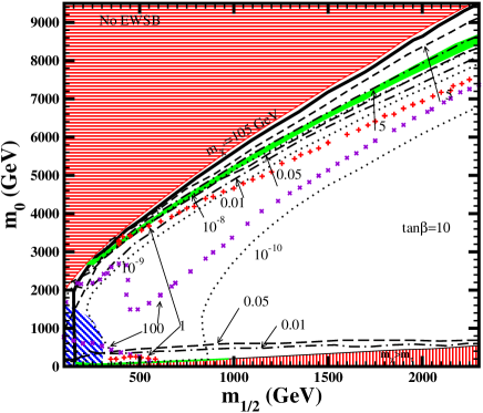
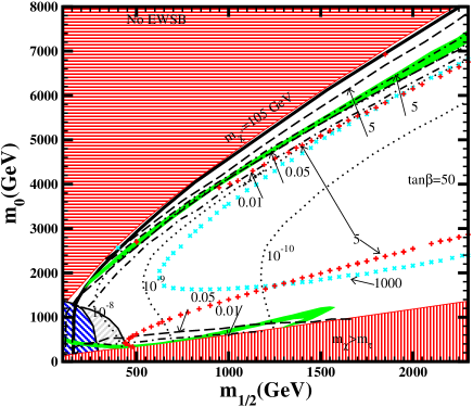
Figure 1: Contours on the $m_{0}-m_{1/2}$ plane, the up and down ruled areas are excluded by the not satisfaction of the EWSB (up) and because $m_{\chi}>m_{\tilde{\tau}}$. The area below the upper thick solid line satisfies the experimental bound on the chargino mass, while the green shaded areas indicate the areas that predict neutralino relic density on WMAP bounds. From left to right, the ruled areas are excluded by the bounds on $m_{h}^{0}$ and $BR(b\rightarrow s\gamma)$ respectively. The doted lines indicates the values of $\sigma_{\chi p}$ in pb, the dash and dot-dash lines corresponds respectively to $2v\sigma_{\chi\chi\rightarrow\gamma\gamma}$ and $v\sigma_{\chi\chi\rightarrow Z\gamma}$ in units of $10^{-29}cm^{3}s^{-1}$. The line of crosses (plus) correspond to the continuum photon production with $E_{\gamma}>1$ GeV ($E_{\gamma}>100$ GeV) also in units of $10^{-29}cm^{3}s^{-1}$.

The lack of experimental evidence of supersymmetric particles leaves us with a number of undetermined parameters in the SUSY models. Therefore, the annihilation cross sections involved in both the computation of $\Omega_{\chi}h^{2}$ and $\gamma$ production can change orders of magnitude with neutralino mass and its gaugino–higgsino composition. To be specific we consider mSUGRA models, where the soft terms of the MSSM are taken to be universal at the gauge unification scale $M_{GUT}$. Under this assumption, the effective theory at energies below $M_{GUT}$ depends on four parameters: the soft scalar mass $m_{0}$, the soft gaugino mass $m_{1/2}$, the soft trilinear coupling $A_{0}$, and the ratio of the Higgs vacuum expectation values, $\tan\beta=\left<H_{u}^{0}\right>/\left<H_{d}^{0}\right>$. In addition, the minimisation of the Higgs potential leaves undetermined the sign of the Higgs mass parameter $\mu$.

To provide some specific values, we assume $A_{0}=0$, $\mu>0$ and two values of $\tan\beta$, 10 and 50. With this two cases we can provide a qualitative picture of most relevant space of parameters and the constraints imposed by phenomenology. The impact of the size of $A_{0}$ or the sign of $\mu$ can be found in several studies of the parameter space of the MSSM (see for example Refs. Cerdeno:2003yt ; Gomez:2005nr ; Gomez:2003cu ; Stark and references therein).

In Fig. 1 we displayed some lines of constant values of $2\left<v\sigma_{\gamma\gamma}\right>$, $\left<v\sigma_{\gamma Z}\right>$ and cross sections for continuum $\gamma-$ray emission on the plane $m_{0}-m_{1/2}$ along with the constraints derived from the lower bound on the mass of the lightest neutral Higgs, $m_{h}^{0}=114.1$ GeV, chargino mass $m_{\tilde{\chi}^{+}}=103$ GeV and BR($b\rightarrow s\gamma$), and the areas with $\Omega h^{2}$ on the WMAP bounds. Also we provide the lines with constant values for the elastic scattering $\chi$–proton, relevant for neutralino direct detection. In the computation we used DarkSUSY Gondolo:2004sc combined with isasugra Paige:2003mg implementing the phenomenological constraints as discussed in Ref. Gomez:2005nr ; the estimation of BR($b\rightarrow s\gamma$) was performed using Refs.  Belanger:2004yn ; Gomez:2006uv .

On the lower area consistent with WMAP the neutralino is Bino–like, the relic density is satisfied mostly due to coannihilations $\chi-\tilde{\tau}$ and in the case of $\tan\beta=50$ because of annihilation $\chi-\chi$ through resonant channels. In this sector $\left<2v\sigma_{\gamma\gamma}\right>$ is dominant by a factor of 10 with respect to $\left<v\sigma_{\gamma Z}\right>$, however its larger values lie in the areas constrained by the bounds on $m_{\tilde{\chi}^{+}}$, $m_{h^{0}}$ and BR($b\rightarrow s\gamma$).

The higher area consistent with WMAP lies on the hyperbolic branch, the neutralino is gaugino–higgsino mixed. The position of this region is very dependent on the mass of the top; we used $m_{t}=175$ GeV.

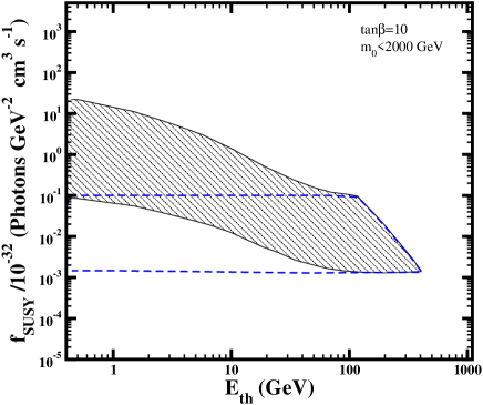
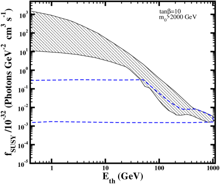
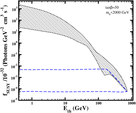
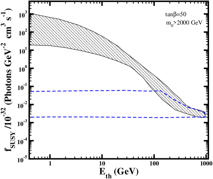
Figure 2: Values of $f_{SUSY}$ respect $E_{th}$, for the points in Fig.1 on the WMAP region and satisfying all the phenomenological constraints. The ruled areas include the continuum $\gamma-$ray emission with $E_{\gamma}>E_{th}$, while the ones limited by thin lines correspond only to monochromatic channels. The left (right) panel corresponds to the upper (lower) allowed WMAP area in Fig. 1.

In Fig. 2 we present the values of $f_{SUSY}$ versus the threshold energy of the detector, starting at $E_{th}=0.4$ GeV, for neutralinos satisfying relic density and phenomenological constraints. $f_{SUSY}$ is calculated as:

$$f_{SUSY}={\theta(E_{th}>m_{\chi})\cdot 2\left<v\sigma_{\gamma\gamma}\right>\over{2m_{\chi}^{2}}}$$

$$+{\theta(E_{th}>m_{\chi}-{m_{Z}^{2}\over{4m_{\chi}}})\cdot\left<v\sigma_{\gamma Z}\right>+~{}k\left<v\sigma_{cont.}\right>\over{2m_{\chi}^{2}}},$$ (4)

where $\theta$ is the step function and $k$ the photon multiplicity for each neutralino annihilation. We display in different panels values of $f_{SUSY}$ corresponding to points on hyperbolic branch ($m_{0}>2$ TeV as we can see in Fig.1) and the values corresponding to the $\chi-\tilde{\tau}$ coannihilation and resonant annihilation areas ($m_{0}<2$ TeV). We can appreciate that on the $\chi-\tilde{\tau}$ coannihilation area, $m_{\chi}$ has an upper bound beyond which the relic density constraint is no longer satisfied while on the hyperbolic branch no upper bound for $m_{\chi}$ is reached. The largest values of $f_{SUSY}$ are not present since they correspond to low values of $m_{1/2}$ suppressed by the bounds on $m_{\tilde{\chi}^{+}}$, $m_{h^{0}}$ and $b\rightarrow s\gamma$. It is interesting to remark that the higher values of $f_{SUSY}$ on the constrained areas lie in which the $\sigma_{\chi-p}$ reaches values in the range of direct detection experiments like Genius Cerdeno:2003yt .

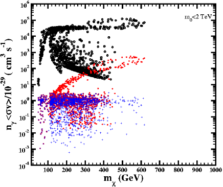
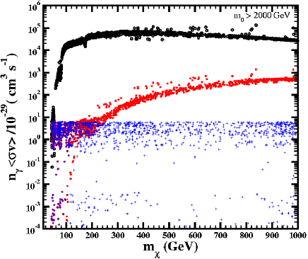
Figure 3: Values of $n_{\gamma}<\sigma_{\chi\chi}v>$ in $cm^{3}/s$ including continuum emission for $E_{\gamma}>1$ GeV (circles), $E_{\gamma}>100$ GeV (stars), and considering only the two monochromatic channels (plus).

To show a more general sampling on the parameter space, we present in Fig. 3 the $\gamma$-ray production in neutralino annihilation versus $m_{\chi}$. Each panel contains about 1400 points satisfying the WMAP and phenomenological constraints mentioned above. These points are selected from random scan over 600000 parameter on the ranges:

$$3< \tan\beta <60,$$

$$50~{}\rm{GeV}< m_{1/2} <2300\,\rm{GeV},$$

$$-3~{}m_{0}< A_{0} <3~{}m_{0},$$

$$50~{}\rm{GeV}< m_{0} <10~{}\rm{TeV},$$ (5)

and both signs of the $\mu$ term.

In the top panel of Fig. 3 we include models with $m_{0}<2$ TeV. These points satisfy the relic density constraint due mostly to $\tilde{\tau}-\chi$ coannihilations, and to a minor extend due to resonances in the annihilation channels (for large values of $\tan\beta$); $m_{\chi}$ remain below $700$ GeV in this panel. The continuum emission dominates for $E_{\gamma}>1$ GeV, while for $E_{\gamma}>100$ GeV we find points where the continuum production is of the same order as the monochromatic $\gamma$’s. The bottom panel of Fig. 3 contains models $m_{0}>2$ TeV. These correspond mostly to the hyperbolic branch region; also we can appreciate that larger values for $m_{\chi}$ are allowed in this area than in the top panel. The points with larger cross sections in both panels corresponds to the smaller values of the pseudo-scalar Higgs mass $m_{A}$ and higher higgsino composition of the neutralino. These two factors favour the fermion production in neutralino annihilation channels. On the top panel, the larger cross sections correspond to the larger values of $\tan\beta$ while on the right panel low values for $m_{A}$ can be reached for any $\tan\beta$.

The mSUGRA results do not differ significantly that the ones obtained in the more general MSSM models obtained by waiving the universality conditions on the soft terms as we will present in section V.2.

II.2 Astrophysics: the $U(\Psi_{0})$ parameter

All the astrophysical considerations are included in the expression $U(\Psi_{0})$ in Eq.(1). This factor accounts for the dark matter distribution, the geometry of the problem and also the beam smearing of the IACT, i.e.

$$U(\Psi_{0})=\int J(\Psi)B(\Omega)d\Omega$$ (6)

where $B(\Omega)d\Omega$ represents the beam smearing of the telescope, commonly known as the Point Spread Function (PSF). The PSF can be well approximated by a Gaussian:

$$B(\Omega)d\Omega=\exp\left[-\frac{\theta^{2}}{2\sigma_{t}^{2}}\right]\sin\theta~{}d\theta~{}d\phi$$ (7)

with $\sigma_{t}$ the angular resolution of the IACT. It is worth mentioning that there is some dependence of $\sigma_{t}$ with the energy (see e.g. IACTparam ). However, for simplicity, we will suppose this term to be constant. The PSF plays a very important role in the way we will observe a possible DM signal in the telescope. However, most of previous works in the literature did not take into account its effect (except Prada04 ; in profumo the PSF apparently was also used, although it is not mentioned in the text (S. Profumo, private communication)). In Section IV we will study in detail the importance of the PSF in the determination of the gamma ray flux profile.

The $J(\Psi)$ factor of Eq.(6) represents the integral of the line-of-sight of the square of the dark matter density along the direction of observation $\Psi$:

$$J(\Psi)=\int_{l.o.s.}\rho_{dm}^{2}(r)~{}d\lambda=\int_{\lambda_{min}}^{\lambda_{max}}\rho_{dm}^{2}[r(\lambda)]~{}d\lambda$$ (8)

Here, $r$ represents the galactocentric distance, related to the distance $\lambda$ to the Earth by:

$$r=\sqrt{\lambda^{2}+R_{\odot}^{2}-2~{}\lambda~{}R_{\odot}\cos\Psi}$$ (9)

where $R_{\odot}$ is the distance from the Earth to the centre of the galactic halo, and $\Psi$ is related to the angles $\theta$ and $\phi$ by the relation $\cos\Psi=\cos\psi_{0}\cos\theta+\sin\psi_{0}\sin\theta\cos\phi$. The lower and upper limits $\lambda_{min}$ and $\lambda_{max}$ in the l.o.s. integration are given by $R_{\odot}\cos\psi\pm\sqrt{r_{t}^{2}-R_{\odot}^{2}\sin^{2}\psi}$, where $r_{t}$ is the tidal radius of the dSph galaxy in this case.

III Dark matter distribution in Draco

In our modelling of Draco we used the sample of 207 Draco stars with measured line-of-sight velocities originally considered as members by wkeg . In selecting these stars these authors relied on a simple prescription going back to Yahil and based on rejection of stars with velocities exceeding $3\sigma_{\rm los}$ where $\sigma_{\rm los}$ is the line-of-sight velocity dispersion of the sample. lokas05 have shown that if all these 207 stars are used to model Draco velocity distribution the resulting velocity moments can be reproduced only by extremely extended mass distribution with total mass of the order of a normal galaxy. Their arguments strongly suggested that some of the stars may in fact be unbound and the simple $3\sigma_{\rm los}$ rejection of stars is insufficient.

Here we apply a rigorous method of removal of such interlopers originally proposed by hartog and applied to galaxy clusters. The method relies on calculating the maximum velocity available to the members of the object assuming that they are on circular orbits or infalling into the structure. The method was shown to be the most efficient among many methods of interloper removal recently tested on cluster-size simulated dark matter haloes by wojtak . Its applicability and efficiency in the case of dSph galaxies was demonstrated by klim . Fig. 4 shows the results of the application of this procedure to Draco. The 207 stars shown in the plot are divided into those iteratively rejected by the procedure (open circles) and those accepted at the final iteration (filled circles).

Figure 4: The line-of-sight velocities versus projected distances from the galaxy centre for 207 stars from wkeg . Open circles mark the 13 stars rejected by our interloper removal procedure, filled circles show the 194 ones accepted.

The final sample with 194 stars is different from any of the three considered by lokas05 therefore we repeat their analysis here for this new selection. Our analysis is exactly the same, except that in the calculation of the velocity moments we use 32-33 stars per bin instead of about 40 and we consider a DM profile with a core in addition to the cusp one. The profiles of the line-of-sight velocity moments, dispersion and kurtosis, obtained for the new sample are shown in Fig. 5. The kurtosis was expressed in terms of the variable $k=[\log(3K/2.7)]^{1/10}$ where $K$ is the standard kurtosis estimator. We assumed that the DM distribution in Draco can be approximated by

$$\rho_{\rm d}(r)=Cr^{-\alpha}{\rm exp}\left(-\frac{r}{r_{\rm b}}\right)$$ (10)

proposed by kmmds , which was found to fit the density distribution of a simulated dwarf dark matter halo stripped during its evolution in the potential of a giant galaxy. In the same work it was found that the halo, which initially had a NFW distribution, preserves the cusp in the inner part (so that $\alpha=1$ fits the final remnant very well) but develops an exponential cut-off in the outer parts. Here we will consider two cases, the profile with a cusp $\alpha=1$ and a core $\alpha=0$. It remains to be investigated which scenarios could lead to such core profiles.

Figure 5: The line-of-sight velocity dispersion (upper panel) and kurtosis variable $k$ (lower panel) calculated for the sample of 194 stars with 32-33 stars per bin. The lines show the best-fitting solutions of the Jeans equations for the DM profile with a cusp (solid lines) and a core (dashed lines).

Figure 6: The best-fitting DM density profiles for Draco with a cusp (solid line) and a core (dashed line).

The best-fitting solutions to the Jeans equations (see lokas05 ) for two component models with dark matter profiles given by (10) are plotted in Fig. 5 as solid lines in the case of the cusp profile and dashed lines for the core. The best-fitting parameters of the two models are listed in Table 1, where $M_{\rm D}/M_{\rm S}$ is the ratio of the total dark matter mass to total stellar mass, $r_{\rm b}/R_{\rm S}$ is the break radius of equation (10) in units of the Sérsic radius of the stars and $\beta$ is the anisotropy parameter of the stellar orbits.

Table 1: Best-fitting parameters of the two-component models for the DM profiles with a cusp ($\alpha=1$) and a core ($\alpha=0$) obtained from joint fitting of velocity dispersion and kurtosis profiles shown in Fig. 5. The last column gives the goodness of fit measure $\chi^{2}/N$.

profile		$M_{\rm D}/M_{\rm S}$		$r_{\rm b}/R_{\rm S}$		$\beta$		$\chi^{2}/N$
cusp		830		7.0		$-0.1$		8.8/9
core		185		1.4		$0.06$		9.5/9

Fig. 6 shows the best-fitting dark matter density profiles in the case of the cusp (solid line) and the core (dashed line). As we can see, both density profiles are similar up to about 1 kpc, where they are constrained by the data. The reason for very different values of the break radius $r_{\rm b}$ in both cases is the following. The kurtosis is sensitive mainly to anisotropy and it forces $\beta$ to be close to zero in both cases. However, to reproduce the velocity dispersion profile with $\beta\approx 0$ the density profile has to be steep enough. In the case of the core it means that the exponential cut-off has to occur for rather low radii, which is what we see in the fit. The cusp profile does not need to steepen the profile so much so it is much more extended and its total mass is much larger.

IV Draco gamma ray flux profiles

In order to compute the expected gamma flux, we need to calculate the value of the “astrophysical factor”, $U(\psi_{0})$, given in Eq.(1) and presented in detail in Section II.2. We calculated it for the core ($\alpha=0$) and cusp ($\alpha=1$) density profiles given by Eq.(10) using the parameters listed in Table 2 (that were deduced from those given in Table 1 and where we used $R_{S}=7.3$ arcmin for Draco, following odenkirchen ). $R_{\odot}$ was set to 80 kpc, as derived from an analysis on the basis of wide-field CCD photometry of resolved stars in Draco aparicio . For the tidal radius we used a value of 7 kpc as given by evans and derived from the Roche criterion supposing an isothermal profile for the Milky Way. Nevertheless, this value depends strongly on the profile used for the Milky Way and Draco, e.g. a value of 1.6 kpc is found when a NFW DM density profile is used for both galaxies evans . It is worth mentioning, however, that we computed $J(\Psi)$ for different values of $r_{t}$ and we checked that the difference between choosing $r_{t}=1.6$ kpc and $r_{t}=7$ kpc is less than 5% for $\Psi=0.5^{\circ}$, and still less than 10% for $\Psi=1^{\circ}$. Therefore, for the case of Draco, any value $r_{t}\gtrsim 1.5$ leads to robust and very similar results.

Table 2: Values of $C$ and $r_{b}$ for a cusp and a core DM density profile given by Eq.(10), as deduced from those parameters listed in Table 1.

profile		$C$		$r_{b}~{}(kpc)$
cusp		3.1 x $10^{7}$ M⊙/kpc2		1.189
core		3.6 x $10^{8}$ M⊙/kpc3		0.238

There is another issue that we will have to take into account in order to calculate $U(\psi_{0})$. If we integrate the square DM density along the line of sight using a cusp DM density profile, we will obtain divergences at angles $\psi_{0}\rightarrow 0$ (clearly there will not be any problem for core profiles). This can be solved by introducing a small constant DM core in the very centre of the DM halo. In particular, the radius $r_{cut}$ at which the self annihilation rate $t_{l}\sim(<\sigma_{ann}v>n_{\chi}~{}r_{cut})^{-1}$ equals the dynamical time of the halo $t_{dyn}\sim(G~{}\overline{\rho})^{-1/2}$, where $\overline{\rho}$ is the mean halo density and $n_{\chi}$ is the neutralino number density, is usually taken as the radius of this constant density core fornengo . For the NFW DM density profile this value for $r_{cut}$ is of the order of $10^{-13}-10^{-14}$ kpc. For steeper DM density profiles (such as the compressed NFW or the Moore profile) a value of $r_{cut}\sim 10^{-8}$ kpc is obtained. We used a value of $10^{-8}$ kpc in all our computations. We must note that $r_{cut}$ represents a lower limit concerning the acceptable values for this parameter, so the obtained fluxes should be taken as upper bounds.

Once we have calculated $U(\psi_{0})$, we will need also to take a value for the $f_{SUSY}$ parameter in order to obtain the absolute flux due to neutralino annihilation (see Eq. 1). We chose a value of $f_{SUSY}=10^{-33}~{}ph~{}GeV^{-2}~{}cm^{3}~{}s^{-1}$ in all our computations for a typical $E_{th}\sim 100$ GeV of the IACT. In the framework of MSSM, this value corresponds to one of the most optimistic values that is possible to adopt for $f_{SUSY}$ according to Fig. 2 for the two different values of tan $\beta$ presented.

The resulting $\gamma$-ray flux profiles for Draco are plotted in Figure 7, where we used a PSF with $\sigma_{t}=0.1^{\circ}$ (to simplify the notation, hereafter we will use PSF$=0.1^{\circ}$ to refer to a PSF with $\sigma_{t}=0.1^{\circ}$). This value of 0.1^∘ is the typical value for an IACT like MAGIC or HESS. It is important to note that the core and a cusp density profiles would be distinguishable thanks to a different and characteristic shape of the flux profile in each case.

Figure 7: Draco flux predictions for the core (dashed line) and cusp (solid line) density profiles, computed for a typical IACT with E${}_{th}=100$ GeV and a PSF$=0.1^{\circ}$. We used $f_{SUSY}=10^{-33}~{}ph~{}GeV^{-2}~{}cm^{3}~{}s^{-1}$ (see text for details).

To illustrate the PSF effect on the shape of the observed flux profile with IACTs, in the top panel of Figure 8 we show the same as in Fig. 7, but here for a PSF$=1^{\circ}$. As we can see, although we have different DM density profiles, a worse telescope resolution makes both resulting flux profiles for a core and a cusp indistinguishable. We may think that we could distinguish them from the value of the absolute flux. However, the difference in the absolute flux between both DM density profiles is very small and in practice the distinction would be impossible. There are many uncertainties in this absolute flux coming from the particle physics. $f_{SUSY}$ may be very different from the most optimistic case assumed here, since it could vary more than three orders of magnitude for this SUSY model (see Fig. 2). On the other hand, the uncertainty in flux due to the DM density profile to be core or cusp is negligible at least in the inner 0.5 degrees.

Figure 8: Top panel: Draco flux predictions for the core (dashed line) and cusp (solid line) density profiles, computed using a PSF$=1^{\circ}$. Bottom panel: Draco flux predictions for the cusp density profile using two different PSFs. Solid line corresponds to PSF=$0.1^{\circ}$ and dashed line to PSF=$1^{\circ}$. The flux profile computing without PSF is also shown for comparison (dot-dashed line).

Concerning the effect of the PSF given the same DM density profile, a worse telescope resolution flattens the flux profile as expected. It can be clearly seen in the bottom panel of Figure 8, where we plot the Draco $\gamma$-ray flux predictions only for the cusp density profile but using two different values of the PSF ($0.1^{\circ}$ and $1^{\circ}$), and where we plot also the same flux profile computed without PSF for comparison.

A good example to show the real importance of the telescope resolution can be found around the controversy generated in the wake of the Draco $\gamma$-ray excess reported by the CACTUS collaboration in 2005 marleau . At this moment, it seems clear that this excess was not real and was probably due to instrumental and trigger-related issues. However, concerning our line of work and always just with the intention of clarifying the role of the PSF, we must mention the results shown in profumo . There, the CACTUS data were superimposed on different flux profiles (each of them related to possible models of DM density profiles for Draco) in Figure 2. These flux profiles were computed using an angular resolution of $0.1^{\circ}$, whereas the CACTUS PSF is quite worse than that (around 0.3^∘ for the Crab and probably worse for Draco profumo ; cactus ). Looking at that figure (despite the authors’ indication to take it with care) one may come to the conclusion that a core profile seems to be the most adequate DM density profile for Draco, as opposed to the cusp profile. However, it would be more appropriate to make this comparison between the CACTUS data and the flux profiles using in both cases the same PSF of the experiment. Doing so and taking into account the PSF effect properly, it would be difficult to use the CACTUS data to discriminate between different models for the DM density profile as described in profumo , since all of the resultant flux profiles would have essentially the same shape. Only the absolute flux could give us a clue to make this distinction possible, but as already mentioned there are too many uncertainties related to an absolute value to be able to extract solid conclusions.

V Detection prospects for some current or planned experiments

V.1 Flux profile detection

Would it be possible to detect a signal due to neutralino annihilation in Draco using present or planned IACTs and satellite-based gamma ray experiments? Although there are many uncertainties concerning both particle physics and astrophysical issues, as already pointed out, it is possible (and necessary) to make some calculations. These calculations will allow us to estimate at least the order of magnitude of the flux that we could expect in our telescopes, and will help us learn which instrument is, in principle, the best positioned and optimised to detect a possible signal from Draco.

Draco is located in the northern hemisphere, more precisely at declination $58^{\circ}$. Because of that, and regarding currently operating IACTs, MAGIC magic and VERITAS veritas are the best options thanks to their geographical position. Since both experiments have comparable sensitivity and PSF, we will focus only on MAGIC. For this IACT, with an energy threshold around 50 GeV for zenith observations, Draco could be observed $61^{\circ}$ above the horizon, so an energy threshold $\sim 100$ GeV seems to be still possible at that altitude.

Concerning GLAST glast , this satellite-based experiment is designed for making observations of celestial gamma-ray sources in the energy band extending from $\sim 10$ MeV to $300$ GeV, which is complementary to the one for MAGIC. Moreover, it will have a PSF $\sim 0.1^{\circ}$ at 10 GeV webglast , which will make this instrument very competitive also in DM searches. GLAST is planned to be launched at the end of 2007.

The flux profiles detection prospects for both gamma-ray experiments can be seen in Figure 9, where the lines of sensitivity for MAGIC and GLAST are superimposed on the flux profile computed using the cusp DM density profile for Draco as given by Eq.(10) together with the parameters listed in Table 2. For the case of MAGIC, the sensitivity line represents 250 hours of observation time and a $5\sigma$ detection level. As pointed out before, this curve should be comparable and valid for VERITAS experiment as well. Concerning the predicted sensitivity for GLAST, it was calculated by the GLAST team webglast for 1 year of observation and a $5\sigma$ detection level. Values of $f_{SUSY}=10^{-33}$ ph GeV^-2 cm³ s^-1 at 100 GeV (MAGIC) and $f_{SUSY}=1\cdot 10^{-29}$ ph GeV^-2 cm³ s^-1 at 1 GeV (GLAST) were chosen to convert the values calculated from the astrophysical factor $U(\Psi_{0})$ to flux. These values of $f_{SUSY}$ correspond to the most optimistic values compatible with that shown in Fig. 2. We chose E${}_{th}=1$ GeV for GLAST to be sure that we will have a good angular resolution for the arriving photons and also to avoid some uncertainties at low energies in the response of the GLAST LAT detector as pointed out in bertone06 .

Figure 9: Draco flux profile detection prospects for MAGIC (top panel) and GLAST (bottom panel). The flux profile (solid line) corresponds to the cusp density profile given in Table 2 and using a PSF=$0.1^{\circ}$. The sensitivity lines for both instruments were computed for a 5$\sigma$ detection level and 250 hours (MAGIC) / 1 year (GLAST) of integration time. These figures should be taken as the most optimistic case, since we used the most optimistic scenario from particle physics in each case. We adopt E${}_{th}=100$ GeV for MAGIC and E${}_{th}=1$ GeV for GLAST. See text for details.

From Figure 9 we can see that the detection of the gamma ray flux profile due to neutralino annihilation in Draco with the MAGIC telescope seems to be impossible (at least for the DM density profiles and the particle physics model used here), since we would need roughly five orders of magnitude more sensitivity than that reached by this instrument in a reasonable time to have at least one opportunity to detect a possible signal coming from DM annihilation. For the case of GLAST we obtain more or less the same, although in this case the expectations are substantially better and we would need three orders of magnitude more sensitivity. We must note that this is the most optimistic scenario, so even leaving space to take into account the large uncertainties coming from the particle physics it seems very hard to have any chance of detection. In fact, in case of adopting a pessimistic value for $f_{SUSY}$, the $\gamma$-ray flux profile shown in Fig. 9 could decrease in more than three orders of magnitude easily.

There are some issues concerning a possible detection of DM annihilation not only in Draco but also in any other possible target that should be taken into account at this moment. In the case of a positive detection, this signal would be diffuse (i.e. no point-like source) for an instrument with a PSF good enough. This fact and the characteristic spectrum of the source represent the best clues to distinguish between a $\gamma$-ray signal due to neutralino annihilation from other astrophysical sources. In the case of Draco, however, we are very far from obtaining any of these clues, so Draco does not seem a good target for DM searches for current or planned $\gamma$-ray experiments (MAGIC-II, for example, will have a factor of 2 more sensitivity than the single MAGIC telescope magic2 , still clearly insufficient, and the same improvement in sensitivity is reached in the case of the GLAST satellite if we observe 5 years instead of 1).

V.2 Excess signal detection

Although it is strongly recommendable to try to detect the gamma ray flux profile due to neutralino annihilation, we could also search only for a gamma ray excess signal in the direction of Draco with a DM origin. In this case the prospects should be somewhat better, since we are only interested in flux detectability (i.e. no interested in observing an extended emission or not; no discrimination between different flux profiles). Draco is around $2^{\circ}$ in the sky (the whole DM halo), and one MAGIC pointing is 4^∘x 4^∘, so the whole galaxy is within one of these MAGIC pointings. This means that, to calculate the prospects of an excess signal detection for MAGIC, we must sum the gamma ray fluxes coming from all the neutralino annihilations that occur in the entire halo of the dSph. The same is valid for the case of GLAST, since one of the main objectives of this mission will be to survey the whole sky, so Draco as a whole will be observed. Nevertheless, most of the $\gamma$-ray flux due to DM annihilation comes from the inner regions of the dwarf, so it would be better to integrate the flux and make all the calculations only for those regions. Otherwise, if we integrate up to very large angles from the center, we would be increasing the noise in a large amount without practically increasing the $\gamma$-ray signal, since the gamma ray flux profile decreases very rapidly from the center to the outskirts.

We would like here to take the opportunity to mention GAW gaw , which is a R&D path-finder experiment, still under development, for wide field $\gamma$-ray astronomy. GAW will operate above 0.7 TeV and will have a PSF $\sim 0.2^{\circ}$. It will consist of three identical telescopes working in stereoscopic mode (80m side). The main goal of GAW is to test the feasibility of a new generation of IACTs, which join high sensitivity with large field of view (24^∘ x 24^∘). GAW is planned to be located at Calar Alto Observatory (Spain) and a first part of the array should be completed and start to operate during 2008. It is a collaborative effort of research Institutes in Italy, Portugal, and Spain. We will also present some calculations concerning the possibility to observe a $\gamma$-ray signal in the direction of Draco by GAW, just to illustrate the capabilities of the instrument. Nevertheless, the main advantages of GAW will point to other directions, e.g. the possibility to survey a large portion of the sky in a reasonable time above 0.7 TeV.

In Table 3 we show the prospects of an excess signal detection ($5\sigma$ level) for MAGIC, GLAST and GAW and for the case of the cusp DM density profile. Both the integrated absolute fluxes for Draco and the values given for the sensitivities (i.e. the minimum detectable flux, $F_{min}$) refer to the inner 0.5^∘ of the galaxy (although the total size of Draco in the sky is $\sim$ 2^∘), just to improve the signal to noise ratio as explained above. The integrated absolute flux for Draco is not the same for the three experiments, since the $f_{SUSY}$ parameter depends on the energy threshold of each instrument, which is different (we chose 100 GeV for MAGIC, 1 GeV for GLAST and 700 GeV for GAW). We did the calculations for the most optimistic case (i.e. the highest value of $f_{SUSY}$ that we could adopt in the MSSM scenario following Fig. 2, and given the energy threshold of each telescope) and the most pessimistic one (the lowest $f_{SUSY}$).

Table 3: Prospects of an excess signal detection for MAGIC, GLAST and GAW. Concerning the integrated flux for Draco, $F_{Draco}$, the most optimistic and pessimistic values are given in the form $F_{Draco,min}$ - $F_{Draco,max}$. $F_{min}$ represents the minimum detectable flux for each instrument. Both the integrated absolute fluxes for Draco and the values given for the sensitivities (i.e. the minimum detectable flux, $F_{min}$) refer to the inner 0.5^∘ of the galaxy (although its size is $\sim$ 2^∘), just to improve the signal to noise ratio as explained in the text.

		$F_{Draco}$ (ph cm-2 s-1)		$F_{min}$ (ph cm-2 s-1)
MAGIC		4.0 x 10-18 - 4.0 x 10-16		2.0 x 10-11 (250 h)
GLAST		4.0 x 10-16 - 4.0 x 10-12		4.0 x 10-10 (1 year)
GAW		2.8 x 10-19 - 2.8 x 10-17		2.2 x 10-12 (250 h)

According to Table 3, an excess signal detection would be impossible with any of these three instruments, since even in the most optimistic cases they do not reach the required sensitivity by far. If we compare these numbers with the maximum fluxes shown in Fig.9, we can see that the enhancement, although relevant (roughly a factor of 4 in the best case), is still very insufficient for a successful detection.

Moreover, from the results shown in Table 3 it becomes really hard to extract any useful results that would help us understand at least a bit better the problem of the dark matter. Indeed, if we observe Draco with MAGIC or GLAST and we do not detect any excess signal, we will not be able to put any useful constraints on the particle physics involved. None of the actual allowed values for $f_{SUSY}$ could be rejected if we find no detection. This makes Draco even less attractive for those current gamma ray experiments that try to find DM traces.

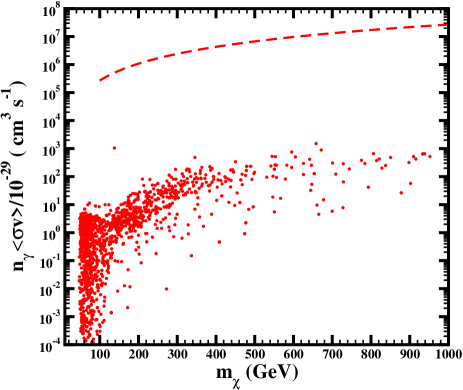
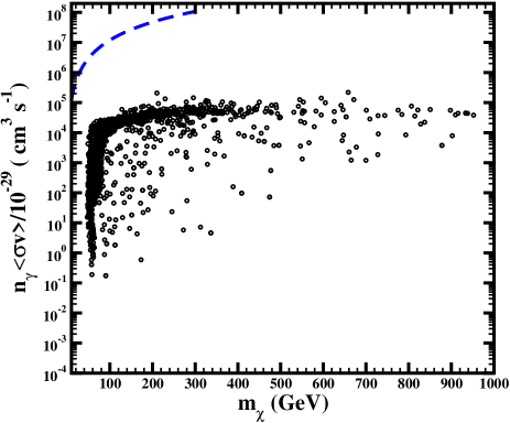
Figure 10: Exclusion limits for MAGIC (upper panel) and GLAST (bottom panel), for continuum $\gamma$-ray emission above 100 GeV (MAGIC) and 1 GeV (GLAST). The lines represent for each instrument the minimum detectable $n_{\gamma}<\sigma v>$ adopting the cusp DM density profile given in Table 2 for Draco. We used 250 hours (1 year) of integration time for MAGIC (GLAST) and a 5$\sigma$ detection level. Below the lines, the SUSY models (points) do not yield a flux high enough for a successful detection. According to these plots, neither MAGIC nor GLAST may put any useful constraints at least to this particular particle physics model.

This can be clearly seen in Fig. 10, where we show the parts of the SUSY parameter space that will be detectable by MAGIC and GLAST for the case of Draco and adopting the cusp DM density profile presented in Section III. The points represent MSSM models, in contrast with Fig. 3 the mSUGRA condition of Eq. 5 has been waived such that models with random sfermion masses below 10 TeV and gaugino masses below 3 TeV are included (we considered equal soft terms for the first two generations to avoid contradiction with flavor violating observables). In the case of MAGIC we only plot those values of $n_{\gamma}<\sigma v>$ computed for $E_{\gamma}>100$ GeV (which is the MAGIC $E_{th}$), and for GLAST only those ones computed for $E_{\gamma}>1$ GeV (GLAST $E_{th}$). We must note that for each case we include in the same figure all the points no matter the value of $m_{0}$ (a distinction was done in Fig. 3). Also, the points related to the monochromatic channels are not shown in both figures, since their values are negligible comparing to those coming from the continuum emission and therefore they are not relevant here.

The limit between the detectable and the non-detectable areas is given by the dashed lines, so that those SUSY points that lie above these lines yield a detectable flux and the points below them are not accessible to observation. As already pointed above, it is clear that the constraints imposed by both experiments to this particular particle physics model (MSSM) are very relaxed and in fact the detection lines do not reach in any case any of the SUSY models by more than two orders of magnitude in the best case. Again, as in Fig. 9, the prospects for GLAST are somewhat better than for MAGIC, but they are still clearly insufficient to extract relevant results or conclusions.

VI Conclusions

In this work we focused on the possibility to detect a signal coming from neutralino annihilation in the Draco dwarf. This galaxy, a satellite of the Milky Way, represents one of the best suitable candidates to search for dark matter outside our galaxy, since it is near and it has probably more observational constraints than any other known dark matter dominated system. This fact becomes crucial when we want to make realistic predictions of the expected observed $\gamma$-ray flux due to neutralino annihilation.

Draco is a dwarf galaxy tidally stripped by the Milky Way, so it seems preferable to build a model for the mass distribution that takes into account this important fact. Using this more appropriate model for Draco, we have obtained the $\gamma$-ray flux profiles for the case of a cusp and a core DM density profiles (both scenarios are equally valid according to the observations). To do that, we first estimated the best-fitting parameters for each density profile by adjusting the solutions of the Jeans equations to velocity moments obtained for the Draco stellar sample cleaned by a rigorous method of interloper removal. Apart from this recommendable and useful update on the best DM model for Draco, one important conclusion can be extracted concerning the absolute $\gamma$-flux: for both cusp and core DM density profiles, the flux values that we obtain are very similar for the inner region of the dwarf, i.e. where we have the largest flux values and signal detection would be easier.

There is, however, a way to distinguish between a core and a cusp DM density profile. The crucial points concerning this issue are the sensitivity and the PSF of the telescope. If the telescope resolution is good enough (and we reach the required sensitivity) a distinction between both cusp and core models may be possible thanks to the shape of the flux profile in each case. However, if the PSF of the instrument is poor, its effect could make it impossible to discriminate between different flux profiles, i.e. different models of the DM density profile. In any case, to be sure that the signal is due to neutralino annihilation, we will need to have a PSF good enough to be able to resolve the source (i.e. we will need to detect with a good resolution at least a portion of the flux profile large enough so we can conclude that it belongs to neutralino annihilation). This fact together with a characteristic spectrum are the unequivocal traces of a DM source. Both issues are of course totally valid not only for Draco but also for any other target, and therefore they should be always taken into account.

We may think that for Draco the effect of the PSF is not especially important, since current experiments do not seem to reach even the required sensitivity to detect a $\gamma$-ray signal coming from the center of the dSph. Indeed, the limiting factor here is the expected flux and not the PSF of the telescope. Nevertheless, we should account for the PSF of the instrument in any case, since we do not know a priori the expected gamma flux and we will not have a realistic prediction unless we include it in our calculations. Only then we will know the exact shape of the flux profile as could be observed by the telescope and therefore we can evaluate the real chances of detection. Furthermore, we must note that the inclusion of the PSF corresponds to a more general analysis not only valid for Draco but also for any target (the case the Milky Way for example where the role of the PSF is critical to understand the origin of the gamma emission in its center).

Some estimations concerning flux profile detection prospects for the MAGIC and GLAST experiments have been also shown. According to these calculations, even in the most optimistic scenario (i.e. with the highest values of $f_{SUSY}$ allowed for the MSSM particle physics model adopted here) a $\gamma$-ray signal detection from Draco seems to be really hard at least for the current IACTs and for the GLAST satellite. In addition, it would be really difficult to improve our expectations for Draco, since for example larger integration times will not improve drastically the sensitivity lines of these instruments up to the level allowing successful detection (we need around five and three orders of magnitude more sensitivity for success with MAGIC and GLAST respectively). The uncertainties coming from astrophysics, as already mentioned, are negligible compared to those coming from the particle physics, so either by choosing a cusp or a core DM density profile for Draco (or even modifying this for a steeper one) we will not be able to increase the $\gamma$-ray flux up to the level where we can expect a signal detection.

We also explored the prospects of an excess signal detection (i.e. we are not interested in the shape of the gamma ray flux profile, only in detectability) for MAGIC and GLAST, but we reached the same strongly negative conclusions as those obtained for the flux profile detection. Both instruments are very far from the required sensitivity so it seems that they do not have any chance of successful detection. But even more, in the case of an (expected) unsuccessful detection we would not be able to put any useful constraints on the particle physics involved (the uncertainties from different dark matter density profiles and other astrophysical considerations are negligible compared to this). None of the actual allowed values for $f_{SUSY}$ could be rejected if we find no detection. This makes Draco even less attractive for those current gamma ray experiments that try to find DM traces.

From these negative results it seems that, at least for current experiments, Draco does not represent a good target for DM searches (although some important enhancements mechanisms in the $\gamma$-ray signal coming from neutralino annihilation in Draco have been proposed in colafrancesco ). If we want to find unequivocal traces of non-barionic dark matter in the Universe, an effort should be done in order to find other more promising DM targets. In this context, it is interesting to note that the number of known dSph galaxies satellites of the Milky Way has increased considerably in the last few years, doing possible that some of them may offer more optimistic detection prospects than Draco itself strigari . A quantitative study should be done in this direction. The search of DM subhalos in the solar neighborhood (see e.g. diemand ) or exploring the IMBHs scenario imbh may represent also other challenging possibilities, although these one more speculative for the moment.

Finally, it is worth mentioning that IACTs that join a large field of view with a high sensitivity will represent the future in this field and will provide a next step in DM searches. In this context, the Cherenkov Telescope Array (CTA) project will be specially important, with a threshold energy well below 100 GeV, a wide spectral coverage up to 100 TeV and a factor of 5-10 more sensitivity than present experiments in the mentioned range. Also GAW, a R&D experiment under development, with an energy threshold $\sim$ 700 GeV and a 24^∘ x 24^∘ field of view, will constitute another complementary attempt in the same direction, although under a different approach.

- (1) Bertone G., Hooper D. and Silk J., 2005, Physics Reports, 405, 279
- (2) Munoz C., 2004, Int. J. Mod. Phys. A, 19, 3093
- (3) Lorentz E. et al., 2004, New Astron. Rev., 48, 339
- (4) Hinton J. A., 2004, New Astron. Rev., 48, 331
- (5) Gehrels N. and Michelson P., 1999, Astropart. Phys., 11, 277
- (6) Kosack K. et al., 2004, ApJ, 608, L97
- (7) Tsuchiya K. et al., 2004, ApJ, 606, L115
- (8) Aharonian F. et al., 2004, A&A, 425, L13
- (9) Albert J. et al., 2006, ApJ, 638, L101
- (10) Spergel D. N. et al., 2007, ApJS, 170, 377
- (11) Bergstrom L. et al., 2005, Phys. Rev. Letters, 95, 241301
- (12) Profumo S., 2006, Physical Review D, 72, 103521
- (13) Aharonian F. et al., 2006, Nature, 439, 695
- (14) Aharonian F. et al., 2006, Phys. Rev. Letters, 97, 221102
- (15) Bergstrom L., 2000, Rep. Prog. Phys., 63, 793
- (16) Evans N. W., Ferrer F. and Sarkar S., 2004, Physical Review D, 69, 123501
- (17) Bergstrom L. and Hooper D., 2006, Physical Review D, 73, 063510
- (18) Mambrini Y., Munoz C., Nezri E. and Prada F., 2006, JCAP, 01, 010
- (19) Colafrancesco S., Profumo S. and Ullio P., 2007, Physical Review D, 75, 023513
- (20) Aharonian F. A., Hofmann F., Konopelko A. K. and Volk H. J., 1997, Astropart. Phys., 6, 343
- (21) Prada F., Klypin A., Flix J., Martínez M. and Simonneau E., 2004, Phys. Rev. Letters, 93, 241301
- (22) Bergstrom L. and Ullio P., 1997, Nucl. Phys. B 504 27
- (23) Bern Z., Gondolo P. and Perelstein M., 1997, Phys. Lett. B 411 86
- (24) Ullio P. and Bergstrom L., 1998, Phys. Rev. D, 57, 1962
- (25) Cerdeno D. G., Gabrielli E., Gomez M. E.and Munoz C., 2003, JHEP, 0306, 030
- (26) Gomez M. E., Ibrahim T., Nath P. and Skadhauge S., 2005, Phys. Rev. D, 72, 095008
- (27) Gomez M. E., Lazarides G. and Pallis C., 2003, Phys. Rev. D, 67 (2003), 097701; Gomez M. E., Lazarides G. and Pallis C., 2002, Nucl. Phys. B, 638, 165
- (28) Stark L. S, Hafliger P., Biland A. and Pauss F., 2005 JHEP, 0508, 059
- (29) Gondolo P., Edsjo J., Ullio P., Bergstrom L., Schelke M. and Baltz E. A., 2004, JCAP, 0407, 008
- (30) Paige F. E, Protopopescu S. D., Baer H. and Tata X., 2003, preprint, hep-ph/0312045.
- (31) Belanger G., Boudjema F., Pukhov A. and Semenov A., 2006, Comput. Phys. Commun., 174, 577 and Comput. Phys. Commun., 2002, 149, 103
- (32) Gomez M. E., Ibrahim T., Nath P. and Skadhauge S., 2006, Phys. Rev. D, 74, 015015
- (33) Profumo S. and Kamionkowski M., 2006, JCAP, 3, 3
- (34) Wilkinson M. I., Kleyna J. T., Evans N. W, Gilmore G. F., Irwin M. J. and Grebel E. K., 2004, ApJ, 611, L21
- (35) Yahil A. and Vidal N. V., 1977, ApJ, 214, 347
- (36) Łokas E. L., Mamon G. A. and Prada F., 2005, MNRAS, 363, 918
- (37) den Hartog R. and Katgert P., 1996, MNRAS, 279, 349
- (38) Wojtak R., Łokas E. L., Mamon G. A., Gottlöber S., Prada F. and Moles M., 2007, A&A, 466, 437
- (39) Klimentowski J., Łokas E. L., Kazantzidis S., Prada F., Mayer L. and Mamon G. A., 2007, MNRAS, 378, 353
- (40) Kazantzidis S., Mayer L., Mastropietro C., Diemand J., Stadel J. and Moore B., 2004, ApJ, 608, 663
- (41) Odenkirchen M., et al., 2001, AJ, 122, 2538
- (42) Aparicio A., Carrera R. and Martinez-Delgado D., 2001, AJ, 122, 2524
- (43) Fornengo N., Pieri L. and Scopel S., 2004, Physical Review D, 70, 103529
- (44) Marleau P., TAUP, September 2005, Zaragoza (Spain); Tripathi M., Cosmic Rays to Colliders 2005, Prague (Czech Republic), September 2005; TeV Particle Astrophysics Workshop, Batavia (USA), July 2005; Chertok M., Proc. of Panic 05, Santa Fe (USA), October 2005
- (45) http://ucdcms.ucdavis.edu/solar2/index.php
- (46) Weekes T. C. et al., 2002, Astropart. Phys., 17, 221
- (47) http://www-glast.stanford.edu/
- (48) Bertone G., Bringmann T., Rando R., Busetto G. and Morselli A., 2006, preprint, astro-ph/0612387
- (49) Baixeras C. et al., 2005, Proc. of the 29th International Cosmic Ray Conference, ICRC, 5, 227
- (50) Maccarone M. C. et al., 2005, Proc. of the 29th International Cosmic Ray Conference, ICRC, 5, 295
- (51) Strigari L. E. Koushiappas S., Bullock J. S., Kaplinghat M., Simon J. D., Geha M. and Willman B., 2007, preprint, astro-ph/0709.1510
- (52) Diemand J., Kuhlen M. & Madau P., 2007, ApJ, 657, 262
- (53) Bertone G.. Zentner A. R. and Silk J., 2005, Physical Review D, 72, 103517
- (54) http://www.mpi-hd.mpg.de/hfm/CTA/CTA_home.html/