Probing the structure of protoplanetary disks: a comparative study of DM Tau, LkCa 15 and MWC 480

Abstract

Context. The physical structure of proto-planetary disks is not yet well constrained by current observations. Millimeter interferometry is an essential tool to investigate young disks.

Aims. We study from an observational perspective the vertical and radial temperature distribution in a few well-known disks. The surface density distribution of CO and HCO⁺ and the scale-height are also investigated.

Methods. We report CO observations at sub-arcsecond resolution with the IRAM array of the disks surrounding MWC 480, LkCa 15 and DM Tau, and simultaneous measurements of HCO⁺ J=1$\rightarrow$0. To derive the disk properties, we fit to the data a standard disk model in which all parameters are power laws of the distance to the star. Possible biases associated to the method are detailed and explained. We compare the properties of the observed disks with similar objects.

Results. We find evidence for vertical temperature gradient in the disks of MWC 480 and DM Tau, as in AB Aur, but not in LkCa 15. The disks temperature increase with stellar effective temperature. Except for AB Aur, the bulk of the CO gas is at temperatures smaller than 17 K, below the condensation temperature on grains. We find the scale height of the CO distribution to be larger (by 50%) than the expected hydrostatic scale height. The total amount of CO and the isotopologue ratio depends globally on the star. The more UV luminous objects appears to have more CO, but there is no simple dependency. The [${}^{13}{\rm CO}$]/[HCO⁺ ] ratio is $\sim 600$, with substantial variations between sources, and with radius. The temperature behaviour is consistent with expectations, but published chemical models have difficulty reproducing the observed CO quantities. Changes in the slope of the surface density distribution of CO, compared to the continuum emission, suggest of a more complex surface density distribution than usually assumed in models. Vertical mixing seems an important chemical agent, as well as photo-dissociation by the ambient UV radiation at the disk outer edge.

1 Introduction

CO rotation line observations of low-mass and intermediate-mass Pre-Main-Sequence (PMS) stars in Taurus-Auriga ($\sim 140$ pc, Kenyon et al.,  1994) provide strong evidences that both TTauri and Herbig Ae stars are surrounded by large ($R_{\mathrm{out}}\sim 200-800$ AU) Keplerian disks (GM Aur: Koerner et al. (1993), GG Tau: Dutrey et al. (1994), MWC 480: Mannings et al. (1997)). Differences between TTauri and Herbig Ae disks are observed in the very inner disk, very close to the star (Dullemond et al., 2001; Monnier & Millan-Gabet, 2002). However, detailed comparisons, namely based on resolved observations instead of SED analysis, between Herbig Ae disks and TTauri disks are too few to allow conclusions about the whole disk. In particular, there is no specific study on the influence of the spectral type on the disk properties. This can be achieved by comparing the properties of outer disks imaged by millimeter arrays.

The first rotational lines of CO (J=1-0 and J=2-1) mostly trace the cold gas located in the outer disk ($R>30$ AU) since current millimeter arrays are sensitivity limited and do not allow the detection of the warmer gas in the inner disk. In the last years, several detailed studies of CO interferometric maps have provided the first quantitative constrains on the physical properties of the outer disks. Among them, the method developed by Dartois et al. (2003) is so far the only way to estimate the overall gas disk structure. Dartois et al. (2003) deduced the vertical temperature gradient of the outer gas disk of DM Tau from a multi-transition, multi-isotope analysis of CO J=1-0 and J=2-1 maps. The dust distribution and its temperature can be traced by IR and optical observations and SED modelling (D’Alessio et al., 1999; Dullemond & Dominik, 2004). However Piétu et al. (2006) recently demonstrated that SED analysis are limited by the dust opacity. Due to the high dust opacity in the optical and in the IR, only the disk surface is properly characterized. Images in the mm domain, where the dust is essentially optically thin, revealed in the case of MWC 480 a dust temperature which is significantly lower than those inferred from SED analysis and from CO images. With ALMA, the method described in this paper, which is today only relevant to the outer disk, will become applicable to the inner disk of young stars.

In this paper, we focus on the gas properties deduced from CO data. The analysis of the millimeter continuum data, observed in the meantime, is presented separately (Piétu et al., 2006)). Here, we generalize the method developed by Dartois et al. (2003) and we apply it to two Keplerian disks surrounding the TTauri star LkCa 15 (spec.type K5, Duvert et al., 2000) and the Herbig Ae star MWC 480 (A4 spectral type, Simon et al., 2000). By improving the method, we also discuss the estimate of disk scale heights. Then, we compare their properties with those surrounding Herbig Ae and TTauri disks such as AB Aur (Piétu et al., 2005), HD 34282 (Piétu et al., 2003), DM Tau (Dartois et al., 2003).

After presenting the sample of stars and the observations in Sect. 2, we describe the improved analysis method in Sect. 3. Results are presented in Sect. 4 and their implications discussed in Sect. 5.

2 Sample of Stars and Observations

2.1 Sample of Stars

The stars were selected to sample the wider spectral type range with only a few objects. Table 1 gives the coordinates and spectral type of the observed stars, as well as of HD 34282 and GM Aur which were observed in ${}^{12}{\rm CO}$ by Piétu et al. (2003) and Dutrey et al. (1998) respectively. Our stars have spectral type ranging from M1 to A0. All of them have disks observed at several wavelengths and are located in a hole or at the edge of their parent CO cloud.

DM Tau:

DM Tau is a bona fide T Tauri star. Guilloteau & Dutrey (1994) first detected CO lines indicating Keplerian rotation using the IRAM 30 meter telescope. Guilloteau & Dutrey (1998) have confirmed those findings by resolving the emission of the ${}^{12}{\rm CO}$ J=1$\rightarrow$0 emission using IRAM Plateau de Bure interferometer (PdBI) and derived physical parameters of its protoplanetary disk and mass for the central star. Dartois et al. (2003) performed the first high resolution multi-transition, multi-isotope study of CO, and demonstrated the existence of a vertical temperature gradient in the disk.

LkCa 15:

This is a CTT isolated from its parent cloud. Duvert et al. (2000) and Qi et al. (2003) observed the disk in ${}^{12}{\rm CO}$ and in HCO⁺. High resolution ${}^{12}{\rm CO}$ data was obtained by Simon et al. (2000) who used it to derive the stellar mass.

MWC 480:

The existence of a disk around this A4 Herbig Ae star was first reported by Mannings et al. (1997). Using data from OVRO, they perform a modelling of the gas disk consistent with Keplerian rotation. More recently, Simon et al. (2000) confirmed that the rotation was Keplerian and measured the stellar mass from the CO pattern.

AB Aurigae:

AB Aur is considered as the proto-type of the Herbig Ae star (of spectral type A0) which is surrounded by a large CO and dust disk. The reflection nebula, observed in the optical, extends far away from the star (Grady et al., 1999). Semenov et al. (2005) used the 30-m to observe the chemistry of the envelope. Piétu et al. (2005) has analyzed the disk using high angular resolution images of CO and isotopologues from the IRAM array and found that, surprisingly, the rotation is not Keplerian. A central hole was detected in the continuum images and in the more optically thin ${}^{13}{\rm CO}$ and ${\rm C}^{18}{\rm O}$ lines.

Table 1: Star properties

Source	Right Ascension	Declination	Spect.Type	Effective Temp.(K)	Stellar Lum.(${\,\rm L}_{\odot}$)	CO paper
LkCa 15	04:39:17.790	22:21:03.34	K5	4350	0.74	1,2
MWC 480	04:58:46.264	29:50:36.86	A4	8460	11.5	1,2
DM Tau	04:33:48.733	18:10:09.89	M1	3720	0.25	3
AB Aur	04:55:45.843	30:33:04.21	A0/A1	10000	52.5	5
HD 34282	05:16:00.491	-09:48:35.45	A1/A0	9440	29	4
GM Aur	04:55:10.98	30:21:59.5	K7	4060	0.74	6

Col. 2,3: J2000 coordinates deduced from the fit of the 1.3 mm continuum map of the PdBI. Errors bars on the astrometry are of order $\leq 0.05^{\prime\prime}$. Col. 4,5, and 6, the spectral type, effective temperature and the stellar luminosity are those given in Simon et al. (2000) and Piétu et al. (2003) for HD 34282 and van den Ancker et al. (1998) for AB Aur. Col.6, list of CO interferometric papers are: 1 = this paper, 2 = Simon et al. (2000), 3 = Dartois et al. (2003), 4 = Piétu et al. (2003), 5 = Piétu et al. (2005), 6 = Dutrey et al. (1998).

2.2 PdBI data

For DM Tau, LkCa 15, and MWC 480, the ¹²CO J=2-1 data were observed in snapshot mode during winter 1997/1998 in D, C2 and B1 configurations. Details about the data quality and reduction are given in Simon et al. (2000) and in Dutrey et al. (1998). The ¹²CO J=2-1 data were smoothed to 0.2 $\,{\rm km.s}^{-1}$ spectral resolution. The HCO⁺ J=1$\rightarrow$0 data were obtained simultaneously: a 20 MHz/512 channels correlator unit provided a spectral resolution of 0.13 $\,{\rm km.s}^{-1}$. The ¹³CO J=1-0 and J=2-1 observations of DM Tau are described in Dartois et al. (2003).

We obtained complementary ¹³CO J=2-1 and J=1-0 (together with C¹⁸O J=1-0 observations) of MWC 480 and LkCa 15. These observations were carried out in snapshot mode (partly sharing time with AB Aur) in winter periods between 2002 and 2004. Configurations D, C2 and B1 were used at 5 antennas. MWC 480 has also shortly been observed in A configuration simultaneously with AB Aur. Finally, data was obtained in the largest A⁺configuration for LkCa 15 and MWC 480 in January 2006 (for a description of these observations, see Piétu et al., 2006). Both at 1.3 mm and 2.7 mm, the tuning was double-side-band (DSB). The backend was a correlator with one band of 20 MHz, 512 channels (spectral resolution 0.11 $\,{\rm km.s}^{-1}$) centered on the ¹³CO J=1-0, one on the C¹⁸O J=1-0 line, and a third one centered on the ${}^{13}{\rm CO}$ J=2$\rightarrow$1 line (spectral resolution 0.05 $\,{\rm km.s}^{-1}$), and 2 bands of 160 MHz for each of the 1.3 mm and 2.7 mm continuum. The phase and secondary flux calibrators were 0415+379 and 0528+134. The rms phase noise was 8$\degr$ to 25$\degr$ and 15$\degr$ to 50$\degr$ at 3.4 mm and 1.3 mm, respectively (up to 70$\degr$ on the 700 m baselines), which introduced position errors of $\leq 0.05\arcsec$. The estimated seeing is about 0.2^′′.

Flux density calibration is a critical step in such projects. The kinetic temperature which is deduced from the modelling is directly proportional to the measured flux density. This is even more problematic since we compare data obtained on several years. Hence, we took great care of the relative flux calibration by using not only MWC 349 as a primary flux reference, assuming a flux S$(\nu)=0.95(\nu/87\mathrm{GHz})^{0.60}$ (see the IRAM flux report 14) but also by having always our own internal reference in the observations. For this purpose we applied two methods: i) we used MWC 480 as a reference because its continuum emission is reasonably compact and bright, ii) we also checked the coherency of the flux calibration on the spectral index of DM Tau, as described in Dartois et al. (2003). We cross-checked all methods and obtained by these ways a reliable relative flux calibration from one frequency to another.

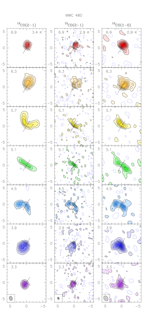
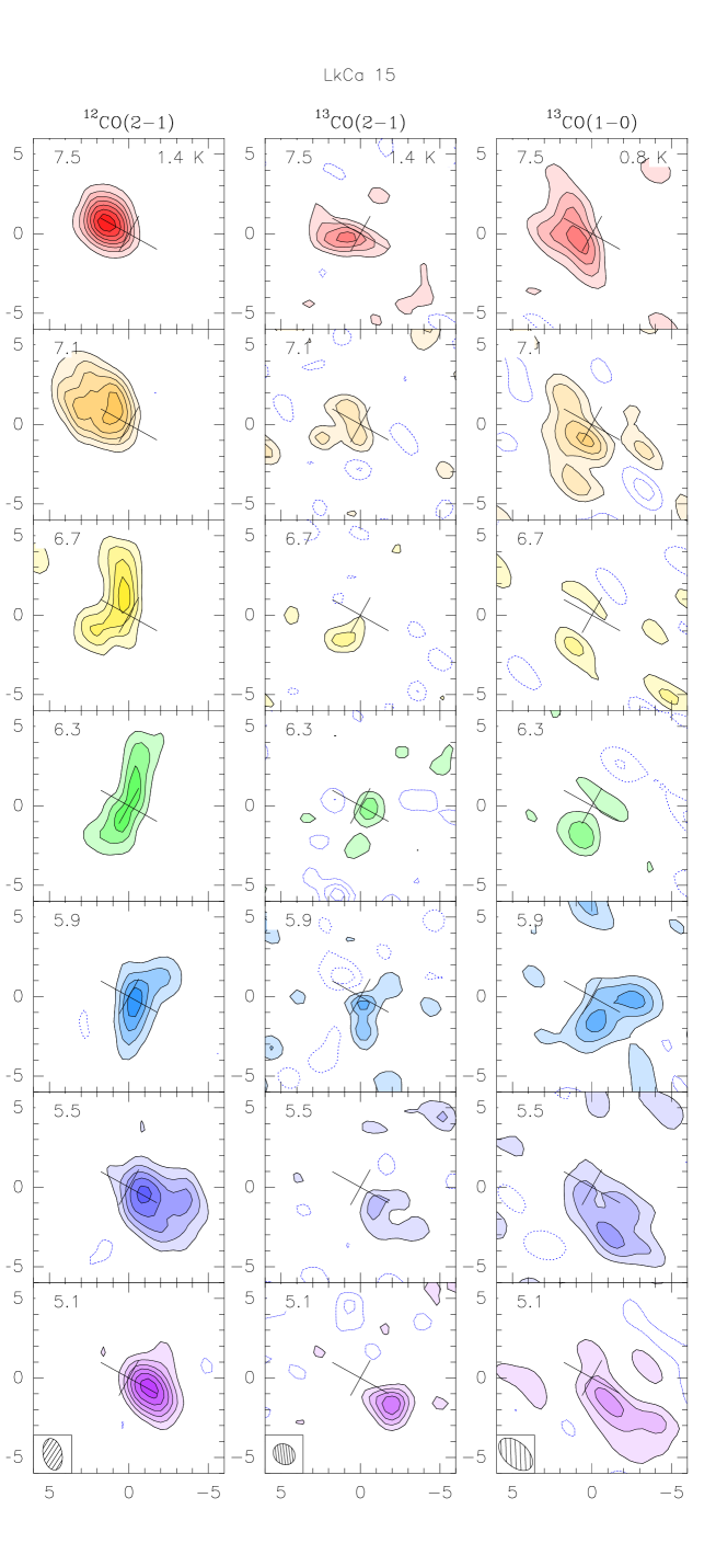
Figure 1: Channel maps of the ${}^{12}{\rm CO}$ and ${}^{13}{\rm CO}$  line emission towards MWC 480 and LkCa 15. The synthesized beam is indicated in each panel. The cross indicates the direction of the major and minor axis of each disk, as respectively derived from the analysis of the line data. The velocity of the channel is indicated in the upper left corner of each panel (LSR velocity in km.s^-1). A 200 m taper has been applied on the ${}^{13}{\rm CO}$ J=2$\rightarrow$1  data of LkCa 15 which where obtained at higher angular resolution. Left: MWC 480 Left: ${}^{12}{\rm CO}$ J=2$\rightarrow$1 line, spatial resolution $1.38\times 0.99^{\prime\prime}$ at PA $16^{\circ}$, contour spacing 200 mJy/beam, or 3.4 K, or 3.6 $\sigma$. Middle: ${}^{13}{\rm CO}$ J=2$\rightarrow$1 line, spatial resolution $0.77\times 0.57$ at PA $26^{\circ}$, contour spacing 50 mJy/beam, or 2.9 K, or 1.9 $\sigma$. Right: ${}^{13}{\rm CO}$ J=1$\rightarrow$0 line, spatial resolution $1.72\times 1.24^{\prime\prime}$ at PA $37^{\circ}$, contour spacing 20 mJy/beam, or 0.9 K, or 1.8 $\sigma$. Negative contours are dashed, and the zero contour is omitted. Right: LkCa 15 Left: ${}^{12}{\rm CO}$ J=2$\rightarrow$1 line, spatial resolution $2.01\times 1.20^{\prime\prime}$ at PA $12^{\circ}$, contour spacing 150 mJy/beam, or 1.4 K, or 2.5 $\sigma$. Middle: ${}^{13}{\rm CO}$ J=2$\rightarrow$1 line, spatial resolution $1.46\times 1.24$ at PA $52^{\circ}$, contour spacing 100 mJy/beam, or 1.4 K, or 1.6 $\sigma$. Right: ${}^{13}{\rm CO}$ J=1$\rightarrow$0 line, spatial resolution $2.55\times 1.51^{\prime\prime}$ at PA $47^{\circ}$, contour spacing 30 mJy/beam, or 0.8 K, or 1.8 $\sigma$. Negative contours are dashed, and the zero contour is omitted.

2.3 Data Reduction and Results

We used the GILDAS software package (Pety, 2005) to reduce the data and as a framework to implement our minimization technique. Figure 1 presents some channel maps of ${}^{12}{\rm CO}$, ${}^{13}{\rm CO}$ J=2$\rightarrow$1 and ${}^{13}{\rm CO}$ J=1$\rightarrow$0 for LkCa 15 and MWC 480. Similar figures for DM Tau can be found in Dartois et al. (2003), and for AB Aur in Piétu et al. (2005). A velocity smoothing to 0.6 $\,{\rm km.s}^{-1}$ (for MWC 480) and 0.4 $\,{\rm km.s}^{-1}$ (for LkCa 15) was applied to produce the images displayed in Fig.1. However, in the analysis done by minimization, we used spectral resolutions of $0.20\,{\rm km.s}^{-1}$ (${}^{12}{\rm CO}$ and HCO⁺) and 0.21 $\,{\rm km.s}^{-1}$ (${}^{13}{\rm CO}$), and natural weighting was retained.

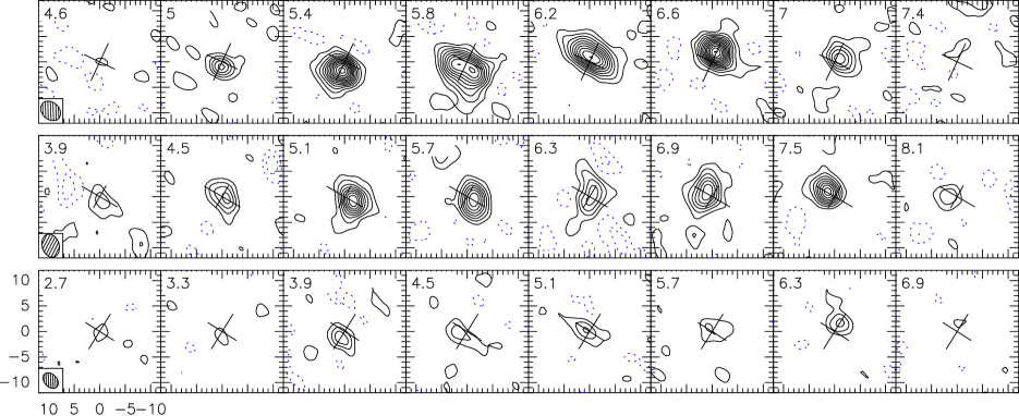
Figure 2: Channel maps of the HCO⁺ J=1$\rightarrow$0 line emission towards DM Tau, LkCa 15 and MWC 480. The cross indicates the direction of the major and minor axis of each disk. The velocity of the channel is indicated in the upper left corner of each panel (LSR velocity in km.s^-1). For displaying purpose, the spectral resolution is 0.6 $\,{\rm km.s}^{-1}$ for MWC 480 and LkCa 15, and 0.4 $\,{\rm km.s}^{-1}$ for DM Tau. All contour steps are 20 mJy/beam ($\sim 2\sigma$), negative contours are dashed and the zero contour is omitted. Top: DM Tau, spatial resolution is $4.3\times 3.3^{\prime\prime}$ at PA $47^{\circ}$, contour step 0.22 K. Middle: LkCa 15, spatial resolution is $4.6\times 3.4^{\prime\prime}$ at PA $19^{\circ}$, contour step 0.25 K. Bottom: MWC 480, spatial resolution is $3.5\times 2.5^{\prime\prime}$ at PA $42^{\circ}$, contour step 0.36 K.

The HCO⁺ images are presented in Fig.2. The typical angular resolution of these images is $3-4^{\prime\prime}$. For LkCa 15, the line flux is compatible with the result quoted by Duvert et al. (2000) and Qi et al. (2003), and for DM Tau with the single-dish measurement of Dutrey et al. (1997).

3 Model description and Method of Analysis

In this section, we summarize the model properties and describe the improvements since the first version (Dutrey et al., 1994).

3.1 Solving the Radiative Transfer Equation

To solve the radiative transfer equation coupled to the statistical equilibrium, we have written a new code, offering non LTE capabilities. More details are given in Pavlyuchenkov et al. (2007). The LTE part, which is sufficient for low energy level of rotational CO lines (J=1-0 and J=2-1), is strictly similar to that of Dutrey et al. (1994), and uses ray-tracing to compute the images. The HCO⁺ data was also analyzed in LTE mode (see Sect.3.2.3 for the interpretation of this assumption). We use a scheme of nested grids with regular sampling to provide sufficient resolution in the inner parts of the disk while avoiding excessive computing time.

3.2 Description of the physical parameters

For each spectral line, the relevant physical quantities which control the line emission are assumed to vary as power law as function of radius (see Sect.3.2.1 for the interpretation of this term) and, except for the density, do not depend on height above the disk plane. The exponent is taken as positive if the quantity decreases with radius:

$$a(r)=a_{0}(r/R_{a})^{-e_{a}}$$

For each molecular line, the disk is thus described by the following parameters :

• $X_{0},Y_{0}$, the star position, and $V_{\mathrm{disk}}$, the systemic velocity.

• PA, the position angle of the disk axis, and $i$ the inclination.

• $V_{0}$, the rotation velocity at a reference radius $R_{v}$, and $v$ the exponent of the velocity law. With our convention, $v=0.5$ corresponds to Keplerian rotation. Furthermore, the disk is oriented so that the $V_{0}$ is always positive. Accordingly, PA varies between 0 and $360^{\circ}$, while $i$ is constrained between $-90^{\circ}$ and $90^{\circ}$ (see fig. 3).

• $T_{\mathrm{m}}$ and $q_{m}$, the temperature value at a reference radius $R_{T}$ and its exponent (see Sect.3.2.3).

• $dV$, the local line width, and its exponent $e_{v}$. The interpretation of $dV$ is discussed in Sect.3.2.6

• $\Sigma_{m}$, the molecular surface density at a radius $R_{\Sigma}$ and its exponent $p_{m}$

• $R_{\mathrm{out}}$, the outer radius of the emission, and $R_{\mathrm{in}}$, the inner radius.

• $h_{m}$, the scale height of the molecular distribution at a radius $R_{h}$, and its exponent $e_{h}$: it is assumed that the density distribution is Gaussian, with

  $$n(r,z)=\frac{\Sigma(r)}{h(r)\sqrt{\pi}}\exp\left[-\left(z/h(r)\right)^{2}\right]$$ (1)

  (note that with this definition, $e_{h}<0$ in realistic disks)

thus giving a grand total of 17 parameters to describe the emission.

It is important to realize that all these parameters can actually be constrained for the lines we have observed, under the above assumption of power laws. This comes from two specific properties of proto-planetary disks: i) the rapid decrease of the surface density with radius, and ii) the known kinematic pattern. The only exception is the inner radius, $R_{\mathrm{in}}$, for which an upper limit of typically 20 – 30 AU can only be obtained.

The use of power laws is appropriate for the velocity, provided the disk self-gravity remains small. Power laws have been shown to be a good approximation for the kinetic temperature distribution (see, e.g. Chiang & Goldreich, 1997), and thus to the scale height prescription. For the surface density, power laws are often justified for the mass distribution based on the $\alpha$ prescription of the viscosity with a constant accretion rate: self-similar solutions to the disk evolution imply power laws with an exponential edge (Hartmann et al., 1998). Although Malbet et al. (2001) pointed out some limitations of this assumption for the inner parts ($r<30$ AU) of the disk, the approximation remains reasonable beyond 50 AU. However, although this may be valid for H₂, chemical effects may lead to significant differences for any molecule. Given the limited spatial dynamic range and signal to noise provided by current (sub-)millimeter arrays, using more sophisticated prescriptions is not yet justified, and power laws offer a first order approximation of the overall molecular distribution.

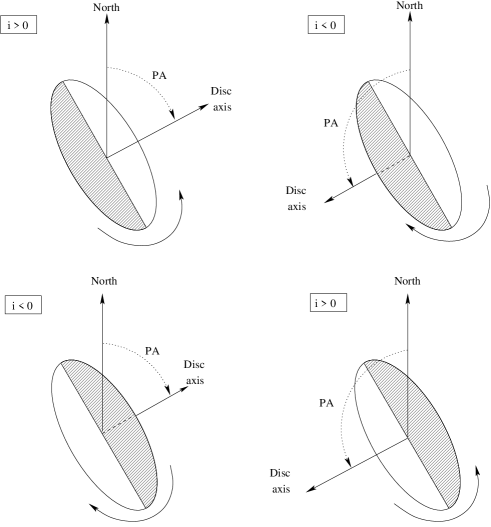
Figure 3: Geometrical convention: four disk configurations yielding the same aspect ratio when projected are presented. The shaded area correspond to the part of the disk that is closer to us than the plane of the sky containing the disk axis. The curved arrow represents the sense of rotation (this defines the disk axis). The projected velocities allow to disentangle between one of the two columns (for the two cases presented on the left, the red-shifted part would be the lower part, and the contrary for the two cases on the right). It is possible to determine the sign of the inclination either with the asymmetry at the systemic velocity if sufficient signal to noise is available, or by other means, e.g. scattered images in the optical and near-IR. PA is classically designed to be positive East from North.

Table 2: Cylindrical vs Spherical description

Line	13CO(1-0)	13CO(2-1)	12CO(2-1)
Cylindrical
$R_{out}$ (AU)	$791\pm 33$	$725\pm 24$	$868\pm 15$
$T_{0}$ (K)	$9.1\pm 0.3$	$14.7\pm 0.3$	$24.2\pm 0.2$
$q$	$-0.17\pm 0.09$	$0.18\pm 0.05$	$0.46\pm 0.01$
$V_{0}$ (km.s-1)	$2.12\pm 0.07$	$2.02\pm 0.06$	$2.09\pm 0.06$
$v$	$0.5$	$0.5$	$0.5$
$dV$ (km.s-1)	$0.133\pm 0.015$	$0.136\pm 0.015$	$0.147\pm 0.010$
$e_{v}$	$-0.28\pm 0.08$	$-0.04\pm 0.07$	$0.08\pm 0.04$
$\Sigma_{m}$ (cm-2)	$26.9\pm 1.7\,10^{16}$	$41.4\pm 6.1\,10^{16}$	$37.4\pm 9.1\,10^{18}$
$p_{m}$	$3.3\pm 0.3$	$3.7\pm 0.4$	$4.5\pm 0.5$
$h_{m}$ (AU)	$27.1\pm 4.4$	$27.8\pm 2.9$	$33.4\pm 2.3$
$e_{h}$	$-1.07\pm 0.20$	$-1.09\pm 0.10$	$-0.99\pm 0.04$
$\chi^{2}$	513329.3	514557.2	136376.5
Spherical
$R_{out}$	$804\pm 34$	$737\pm 20$	$898\pm 12$
$T_{0}$	$9.3\pm 0.3$	$15.2\pm 0.4$	$26.7\pm 0.2$
$q$	$-0.14\pm 0.09$	$0.20\pm 0.05$	$0.50\pm 0.01$
$V_{0}$ (km.s-1)	$2.16\pm 0.07$	$2.07\pm 0.06$	$2.08\pm 0.05$
$v$	$0.5$	$0.5$	$0.5$
$dV$ (km.s-1)	$0.135\pm 0.016$	$0.137\pm 0.015$	$0.183\pm 0.012$
$e_{v}$	$-0.26\pm 0.08$	$-0.05\pm 0.06$	$0.17\pm 0.05$
$\Sigma_{m}$ (cm-2)	$25.7\pm 1.8\,10^{16}$	$35.1\pm 5.3\,10^{16}$	$41.1\pm 7.4\,10^{17}$
$p_{m}$	$3.2\pm 0.3$	$3.6\pm 0.4$	$3.4\pm 0.4$
$h_{m}$ (AU)	$20.7\pm 2.2$	$23.4\pm 2.4$	$19.7\pm 1.4$
$e_{h}$	$-1.32\pm 0.18$	$-1.13\pm 0.12$	$-1.25\pm 0.06$
$\chi^{2}$	513329.5	514558.9	136451.5

Results for DM Tau with “free” scale-height and “free” line-width (see Sect. 3.2.5 and 3.2.6 for more details) in the cylindrical and spherical representations. Caution: this table is here to illustrate the dependence on the geometry of as many parameters as possible. The best parameters to be applied to DM Tau should be taken from Table 3.

3.2.1 Spherical vs Cylindrical representation

To describe the disk and its parameters, we can use either cylindrical or spherical coordinates.

The description given in the previous sub-section is unambiguous for thin disks (where $h(r)\ll r$), However, for molecular disks with outer radius as large as 800 AU, the disk thickness is no longer small, and the classical theory of hydrostatic scale height, which uses cylindrical coordinates, is only valid in the small $h/r$ limit. It may then become significant to distinguish between a spherical representation, where the functions depends on the distance to the star ($r=d$) and height above disk plane, $z$

$$F=f(d,z)$$ (2)

and a cylindrical representation, where the functions depends on the projected distance on the disk ($r=\rho$) and height $z$

$$F=f(\rho,z)$$ (3)

with $d^{2}=\rho^{2}+z^{2}$. It is obvious that the exponent of the power laws will depend slightly on which description is selected. We have evaluated the differences between the two different representations (see Tab.2): as expected, the results are very similar for  ${}^{13}{\rm CO}$, but the cylindrical representation is a $\sim$ 8 sigma better representation for  ${}^{12}{\rm CO}$ J=2$\rightarrow$1  (the most affected transition because of its higher opacity). The most affected parameters are $\Sigma$ and $h$. However, with the exception of the scale height, the effects remain small compared to the uncertainties. Accordingly, we have arbitrarily decided to represent all parameters in terms of cylindrical laws, i.e. the radius is $r=\rho$ in the model description.

3.2.2 Reference Radius

Unless $p_{m}\simeq 0$, the choice of the reference radius $R_{\Sigma}$ will affect the relative error bar on $\Sigma_{m}$, $\delta\Sigma_{m}/\Sigma_{m}$. Depending on the angular resolution and on the overall extent of the emission, for each molecular line, there is a different optimal radius $R_{\Sigma}$ which minimizes this relative error. The same is true for all other reference radii for the power laws. This makes direct comparison at an arbitrary radius not straightforward. To circumvent this problem, we have determined $\Sigma_{m}$, $\delta\Sigma_{m}$ as a function of the reference radius for each transition, and selected the $R_{\Sigma}$ giving the best S/N ratio. Results are given Fig.4-6: note that the curves $\Sigma_{m}(R_{\Sigma})$ should not be interpreted as independent estimates of the local surface density at different radii: they explicitly rely on the assumption of a single power law throughout the whole disk.

The same arguments can be applied to all other power laws, in particular to the scale height and the temperature. However, for the latter, the exponent is usually small ($q=-0.2-0.5$), so the choice of the reference radius is less critical. Figure 4 shows the variation of the parameters (here $\Sigma_{m}$, $T_{m}$ and $h$) and of the signal to noise ratio as a function of the reference radius for DM Tau. This is a reanalysis of the data published by Dartois et al. (2003). This method gives consistent results with previous work, but allows a more precise determination of the parameters (especially the surface density as stated above), by determining in which region they are constrained. Fig.4 indicates that the temperature is determined around 100 – 200 AU, while the surface densities are constrained in the 300 – 500 AU region. Somewhat smaller values apply to the other sources, LkCa 15 and MWC 480 (see Fig.5-6).

3.2.3 Temperature law

The interpretation of $T_{m}$ (and as a consequence of $\Sigma_{m}$) depends on the specific model of radiative transfer being used. In this paper, we are dealing with CO isotopologues, for which LTE is good approximation: $T_{m}$ is then the kinetic temperature. For transitions which may not be thermalized, two different radiative transfer models may be used. We can apply an LTE approximation: since we are fitting brightness distributions, $T_{m}$ is in this case the excitation temperature $T_{\mathrm{ex}}$, and the surface density $\Sigma_{m}$ is computed assuming the same temperature controls all level population, i.e. the partition function. We can also solve for molecular line excitation using a non-LTE statistical equilibrium code: $T_{m}$ is then the kinetic temperature, and $\Sigma_{m}$ the total molecule surface density, within the limitations of the radiative transfer code accuracy. In this paper, only the LTE mode was used.

3.2.4 Surface Density

The surface density is expected to fall off rapidly with distance from the star ($p(\mathrm{H}_{2})\simeq 1-2$), and in particular much more rapidly than the temperature ($q\simeq 0.5$). Remembering that, because of the partition function, the line opacity of a $J=1-0$ transition scales as $\Sigma_{m}/T^{2}$ at high enough temperatures (for constant line width), this indicates that, in general, the central part of the disk is much more optically thick than the outer regions. For the detectable lines, the temperature can be derived from the emission from this optically thick core, while the surface density $\Sigma_{m}$ is derived from the optically thin region. This remains valid provided the same temperature law applies to the two regions. For the weakest lines, the optically thick core may be too small, and the temperature exponent remains essentially unconstrained: this should be reflected to by the error bars on the temperature. In such cases, however, the line emission scales as $\Sigma_{m}/T$ (for J=1-0 line).

If the molecule is very abundant, such as CO, the local line core may be optically thick almost throughout the disk. However, the local line wings remain optically thin: if the velocity resolution is high enough, this information can be used to constrain the opacity, and hence the surface density, although less accurately. To illustrate this point, let us consider the case of a face on disk. The apparent width of the line profile is then controlled only by the internal velocity dispersion (turbulent + thermal) and by the line opacity. In the outer parts, the line is optically thin and of Gaussian shape, while in the inner parts, the line is broadened by the large opacity, and the profile tends towards a square shape, with width proportional to $\sqrt{\ln(\tau)}$. The evolution of the line profiles as function of radius indicates at which radius $\tau=1$, and thus constrains the molecular surface density. Note that if the spectral resolution is insufficient to properly sample the line width, this is no longer possible. Current correlators are not instrumentally limited but smoothing can be necessary when the sensitivity is the limiting factor. If the disk is not seen face on, the systematic velocity gradient get superimposed to this local line broadening, but does not change the fundamental relationship between the apparent (local) line width and the opacity. In any case, since the effect goes as $\sqrt{\ln(\tau)}$, measuring the surface density by such a method is expected to be rather unprecise, and will result in larger errors. Furthermore, it should be noted that this opacity broadening effect results in a slight coupling of the line width parameters, $dV$ and $e_{v}$, to the surface density.

3.2.5 Scale Height

The existence of a known kinematic pattern also allows to constrain the scale height parameters $h_{0}$ and $e_{h}$. Unless the disk is seen face on, for an optically thin line, the velocity range intersected along a line of sight will depend on the disk inclination and flaring, resulting in a coupling between scale height and line width. For an optically thick line, the difference in inclinations between the front and back regions of the disk can also be measured. The spatial distribution of the emission as a function of projected velocity (or function of the velocity channels) along the line of sight will depend on the scale height of the disk (this is illustrated for the opacity by Fig.3 from Dartois et al. (2003)). At first glance, the expected scale heights, of order 50 AU at 300 AU from the star, would appear too small compared to the resolution of $0.7-1.5^{\prime\prime}$ (100 to 200 AU), and the exponent $e_{h}$ even more difficult to constrain. However, millimeter interferometry, being an heterodyne technique, allows phase referencing between velocity channels, and the precision in relative positions is equal to the spatial resolution divided by the Signal to Noise (as our bandpass accuracy, about a degree, is not the limiting factor), i.e. $\sim 10$ AU. This super-resolution approximately matches the expected displacements due to Keplerian rotation,

$$\delta r=2r\frac{\delta v}{v}\simeq 10\leavevmode\nobreak\ \mathrm{AU\leavevmode\nobreak\ at}\leavevmode\nobreak\ r=100\leavevmode\nobreak\ \mathrm{AU}$$ (4)

for $\delta v=0.15\,{\rm km.s}^{-1}$. Note that in Eq.4, the value to be used for $\delta v$ is approximately the largest of the local line width and the spectral resolution. As a result, the scale height has a measurable effect on the images, even though the flaring parameter is difficult to constrain.

Actually, because of the effect of the scale height on the disk images, if a simple hydrostatic equilibrium is assumed instead of handling the scale height separately, it will result in a bias in the temperature law since one is then introducing a coupling between the vertical distribution of the molecules and the temperature which is vertically isothermal in our model.

Finally, note that because the derivation of the scale height depends on the differing inclinations of the optically thick parts, there is also a coupling between the surface density and the scale height derivation. This coupling is specially strong for disks close to edge-on.

3.2.6 Line Width

Line broadening results from a combination of thermal and turbulent velocities.

$$\Delta V=\sqrt{\frac{2kT}{m}+v_{\mathrm{turb}}^{2}}$$ (5)

However, an accurate representation of the thermal broadening requires a correct fitting of the gas temperature. This can become problematic when dealing with lines which are sub-thermally excited. Accordingly, our code offers two different parameterizations of the line width. The first one is

$$\Delta V=\sqrt{\frac{2kT}{m}+dV^{2}}\mathrm{\leavevmode\nobreak\ \leavevmode\nobreak\ i.e.\leavevmode\nobreak\ \leavevmode\nobreak\ }dV=v_{\mathrm{turb}}$$ (6)

which corresponds, for $e_{v}=0$ ($v_{\mathrm{turb}}=cte$), to the parametrization used in our previous papers. The second one is

$$\Delta V=dV=dV_{m}(r/R_{dV})^{-e_{v}}$$ (7)

i.e., we do not separate the thermal component from the total line width. This offers the advantage of providing values which are not biased when the kinetic temperature is difficult to constrain (as can happen for lines which are not at LTE). We use this new description in this paper.

Note that all line widths we quote are half-width at $1/e$. This allows direct comparison with the thermal velocity, $\sqrt{2kT/m}$, but one should multiply by $2\sqrt{\ln(2)}=1.66$ to convert to FWHM. As described before, the line width is also coupled to the scale height.

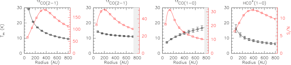
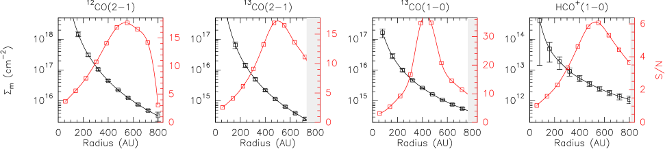
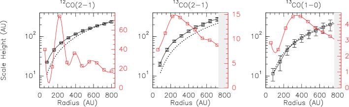
DM Tau

Figure 4: From left to right ${}^{12}{\rm CO}$ J=2$\rightarrow$1, ${}^{13}{\rm CO}$ J=2$\rightarrow$1, ${}^{13}{\rm CO}$ J=1$\rightarrow$0  and HCO⁺  J=1$\rightarrow$0  in DM Tau. Top: Temperature $T_{\mathrm{m}}$ (black curve, left axis) and signal to noise on the temperature $T_{\mathrm{m}}/\delta T_{\mathrm{m}}$ (grey curve, right axis) as a function of reference radius $R_{T}$.Middle Surface density $\Sigma_{m}$ (left axis) and signal to noise on the surface density $\Sigma_{m}/\delta\Sigma_{m}$ (right axis) as a function of reference radius $R_{\Sigma}$. Bottom Scale height $h$ (left axis) and signal to noise on the scale height $h/\delta h$ (right axis) as a function of reference radius $R_{h}$.

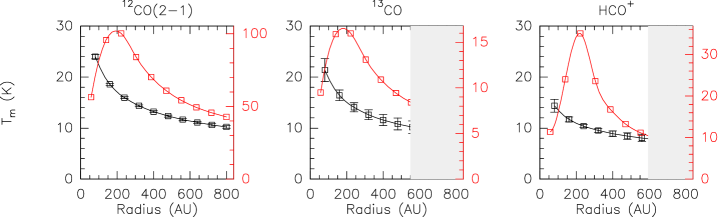
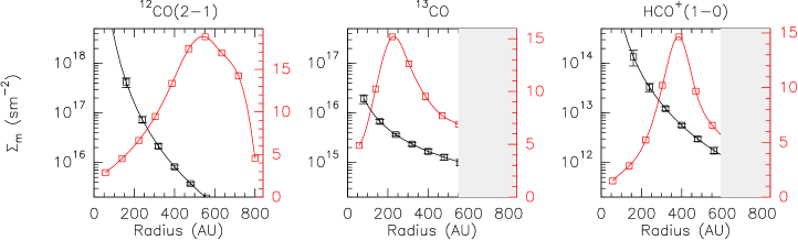
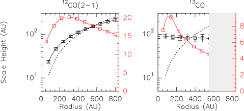
LkCa 15

Figure 5: From left to right ${}^{12}{\rm CO}$, ${}^{13}{\rm CO}$  and HCO⁺  J=1$\rightarrow$0  in LkCa 15. Top: Temperature $T_{\mathrm{m}}$ (black curve, left axis) and signal to noise on the temperature $T_{\mathrm{m}}/\delta T_{\mathrm{m}}$ (grey curve, right axis) as a function of reference radius $R_{T}$.Middle Surface density $\Sigma_{m}$ (left axis) and signal to noise on the surface density $\Sigma_{m}/\delta\Sigma_{m}$ (right axis) as a function of reference radius $R_{\Sigma}$. Bottom Scale height $h$ (left axis) and signal to noise on the scale height $h/\delta h$ (right axis) as a function of reference radius $R_{h}$. For HCO⁺   the temperature and surface density were adjusted separately: the curves should be used as an indicator of the region over which these values are actually constrained, but not as a quantitative measure in terms of S/N, as the coupling between temperature and surface density is ignored.

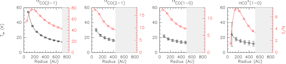
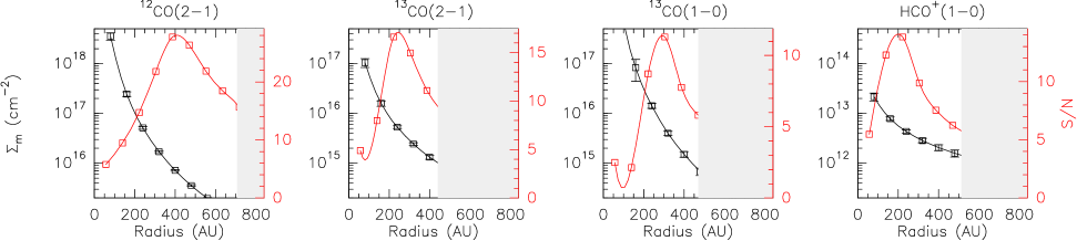
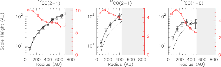
MWC 480

Figure 6: From left to right ${}^{12}{\rm CO}$ J=2$\rightarrow$1, ${}^{13}{\rm CO}$ J=2$\rightarrow$1, ${}^{13}{\rm CO}$ J=1$\rightarrow$0  and HCO⁺  J=1$\rightarrow$0 in MWC 480. Top: Temperature $T_{\mathrm{m}}$ (black curve, left axis) and signal to noise on the temperature $T_{\mathrm{m}}/\delta T_{\mathrm{m}}$ (grey curve, right axis) as a function of reference radius $R_{T}$.Middle Surface density $\Sigma_{m}$ (left axis) and signal to noise on the surface density $\Sigma_{m}/\delta\Sigma_{m}$ (right axis) as a function of reference radius $R_{\Sigma}$. Bottom Scale height $h$ (left axis) and signal to noise on the scale height $h/\delta h$ (right axis) as a function of reference radius $R_{h}$. As for LkCa 15, temperature and surface density are adjusted separately for HCO⁺.

3.3 Minimization Technique

Using the disk parametrization described above, we have improved several aspects of the method originally developed by Dartois et al. (2003).

3.3.1 Minimization Method and Error Bars

The comparison between model and data and the $\chi^{2}$ minimization is always performed inside the UV plane, using natural weighting (Guilloteau & Dutrey, 1998). We have implemented a modified Levenberg-Marquardt minimization scheme to search for the minimum, and we use the Hessian to derive the error bars. This scheme is much faster than the grid search technique used previously, and less prone to local minima. It allows to fit simultaneously more parameters, and thus provide a better estimates of the errors because the coupling between parameters is taken into account.

However, the current fit method does not handle asymmetric error bars which happen in skewed distributions: this limitation should not be ignored when considering the errors on $\Sigma$, $T$ or $R_{\mathrm{out}}$. The quoted error bars include thermal noise only, but do not include calibration errors (in phase and in amplitude). Amplitude calibration errors will directly affect the absolute values of the temperature or the surface density (as a scaling factor, but not the exponent) while phase errors can introduce a seeing effect. The latter effect is very small for line analysis because molecular disks are large enough but it starts to be significant for dust disks. Our careful calibration procedure brings the amplitude effect to below 10 %. All other parameters are essentially unaffected by calibration errors.

3.3.2 Continuum Handling

The speed improvement allowed us to treat more properly the continuum emission. Even though the continuum brightness is small compared to the line brightness, continuum emission cannot be ignored when trying to retrieve parameters from the line emission because it appears systematically in all spectral channels.

A simultaneous fit of the continuum emission with its own physical parameters will properly take into account these biases. We performed this by adding to the spectral $UV$ table a channel dedicated to the continuum emission. The global $\chi^{2}$ is given by the sum $\chi^{2}=\chi^{2}_{C}+\chi^{2}_{L}$ where $\chi^{2}_{C}$ and $\chi^{2}_{L}$ are the $\chi^{2}$ for the continuum and for the line minimization, respectively. The continuum emission is fitted using the following parameters: $R_{Cint}$, $R_{Cout}$, the inner and outer radii of the dust distribution, $\Sigma_{d}$ and $p_{d}$, the surface density power law, and $T_{d}$ and $q_{d}$, the dust temperature power law. Note that the representation of the continuum needs only be adequate within the noise provided by the spectral (total) line width, about 10 to 20 MHz, rather than for the whole receiver bandwidth (600 MHz). A simplified model is thus often acceptable, as shown below.

We also compared this robust method with a simplified (and faster) one in which we subtract, inside the $UV$ plane, the continuum emission from the line emission before fitting. This subtraction is not perfect: for the optically thick regions (which always occupy some fraction of the line emission) continuum should not be subtracted. However, unless the disk is seen face on, because of the Keplerian shear, at each velocity, the line emitting/absorbing region only occupies a small fraction of the disk area. This fraction is at most of order of the ratio of the local line width to the projected rotation velocity at the disk edge, in practice less than 10 – 15 % for the disks we considered. Accordingly, the error made by subtracting the whole continuum emission in every channel is quite small.

We verified that this simplified method gives, as expected, the same results as the robust one. We used it, as it is significantly faster. This better handling of the continuum allowed us to improve on the mass determination of MWC 480 (Simon et al., 2000), where the continuum is relatively strong.

3.3.3 Multi-Line fitting

The code has also been adapted to allow minimization of more than one data set at a time. This has been used to simultaneously fit the ${}^{13}{\rm CO}$ J=1$\rightarrow$0 and J=2$\rightarrow$1 transitions. For multi-line fitting, the temperature is derived from the line ratio. The temperature is determined in the disk region where both lines are optically thin. In this case, the fit is much more accurate than from a single line observation if there is no significant vertical temperature gradient. When a temperature gradient is present, the derived temperature will reflect an “average” temperature weighted by the thermal noise.

4 Results

4.1 Interpretation of the Power Law model

The parametric model would perfectly describe the line emission from a molecule in LTE in a vertically isothermal disk which is in hydrostatic equilibrium, with power law for the kinetic temperature and surface density, and constant molecular abundance. In such a case, $e_{v}=q/2$ if the local line width is thermal, and $h=q/2-1-v$ and $h_{0}=(\sqrt{2kT_{0}/\overline{m}})/V_{0}$ (using the same reference radius $R_{h}=R_{T}=R_{v}$, $\overline{m}$ being the mean molecular weight). If such a disk was chemically homogeneous, all molecular lines would yield the same results for the 17 parameters (after correction of $\Sigma_{m}$ for the molecule abundance). Differences between the parameters derived from several transitions will reflect departures from such an ideal situation.

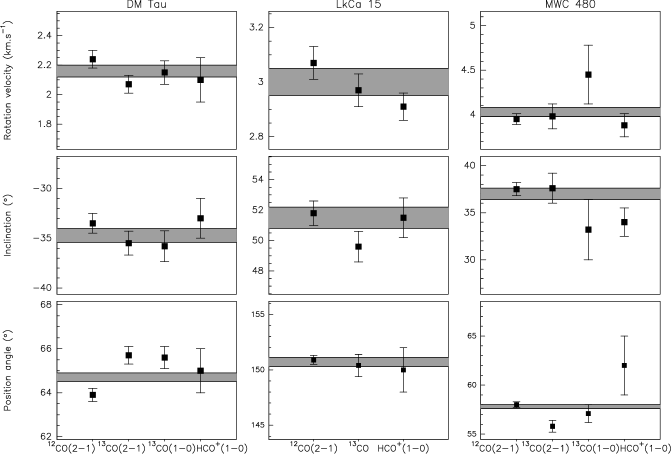
Figure 7: From left to right: kinetic and geometric parameters derived for DM Tau, LkCa 15 and MWC 480. From top to bottom: rotation velocity at 100 AU, inclination and position angle. For DM Tau and MWC 480, the error bars represent (from left to right) the value of the parameter measured from the ${}^{12}{\rm CO}$ J=2$\rightarrow$1, ${}^{13}{\rm CO}$ J=2$\rightarrow$1, ${}^{13}{\rm CO}$ J=1$\rightarrow$0  and HCO⁺  J=1$\rightarrow$0  lines. For LkCa 15 (from left to right), the values are derived from the ${}^{12}{\rm CO}$ J=2$\rightarrow$1  line, from the simultaneous fit of the ${}^{13}{\rm CO}$ J=2$\rightarrow$1  and the ${}^{13}{\rm CO}$ J=1$\rightarrow$0  lines, and from the HCO⁺  J=1$\rightarrow$0  line. In all three sources, the grey area represent $\pm 1\sigma$ around the mean of the values of the CO isotopes.

For example, the geometric parameters PA and $i$ should all be identical, as should be the kinematic parameters $V_{\mathrm{disk}},V_{0},v$ (and we should have $v=0.50$ for Keplerian rotation). $X_{0},Y_{0}$ should reflect the absolute astrometric accuracy of the IRAM interferometer. Different values for $T_{m}$ from several transitions for the same molecule, or its isotopologues, may reveal vertical temperature gradients, or, in case of non-LTE excitation, density gradients, since such transitions probe different regions of the disk. The values of $T_{m}$ from different molecules may also provide constraints on the density, because of the different critical densities. And, more directly, the values of $\Sigma_{m}$, $p_{m}$, $R_{\mathrm{in}}$ and $R_{\mathrm{out}}$ will reflect the chemical composition of the disk as function of radius.

4.2 Geometric and kinematic parameters

Figure 7 shows the geometric and kinematic parameters PA, $i$ and rotation velocity $V_{100}$ derived from the observed transitions in DM Tau, LkCa 15 and MWC 480. The grey area represent the 1 $\sigma$ range of the mean value computed from the CO lines. As expected, the derived value are in very good agreement altogether. In particular, the distribution of the derived values and the error bars are consistent with a statistical scattering, meaning that: i) the observed lines come from the same disk, ii) the error bars have the good magnitude, and iii) there is no bias in the determination of the parameters. This analysis of the “basic” parameters is of prime interest, because it shows that the analysis method is robust, and that the error bars have a real physical meaning. Although noisier, the kinematic and geometric parameters determined from HCO⁺   are in agreement with those found from CO. We thus used the CO-derived values to determine the surface density and excitation temperature of HCO⁺ .

4.3 Results

Tables 3, 4 and 5, present the best fit results for DM Tau, LkCa 15 and MWC 480, respectively. Compared to previous papers (e.g. Simon et al., 2000; Duvert et al., 2000; Dutrey et al., 1998), the new fits include all the refinements of the method described in Sec.3 and in Piétu et al. (2006).

All quoted results where obtained using cylindrical coordinates and the continuum was subtracted to the spectroscopic data before analysis. All the models were obtained in the same manner. In particular, we assumed a constant line width ($e_{v}=0$), Keplerian rotation ($v=0.5$), and a flaring exponent $e_{h}=-1.25$ (the value for a Keplerian disk in hydrostatic equilibrium with a temperature radial dependence of 0.5). This value is very close to those found by Chiang & Goldreich (1997) for the super heated layer model. Systematic tests with different sets of free parameters ensure that the geometrical and kinematical parameters are insensitive to these assumptions. The temperature $T_{m}(r)$ is also hardly affected. The surface density $\Sigma_{m}(r)$ and outer radius $R_{out}$ depends to some extent on the assumed flaring parameter $e_{h}$. However, because of the coupling between scale height and line width, both $H_{0}$ and $dV$ should be taken with some caution. The dynamical mass derived from ${}^{12}{\rm CO}$ also depends weakly on the assumed scale height, since we derive the inclinations from the apparent CO surface.

The differences between the values reported here for DM Tau and those published by Dartois et al. (2003) come from the different assumptions in the analysis. Dartois et al. (2003) assumed hydrostatic equilibrium, and model the line width following Eq.6 . They also assumed [${}^{12}{\rm CO}$]/[${}^{13}{\rm CO}$] = 60.

Table 3: Best parameters for DM Tau.

(1)	(2)	(3)	(4)	(5)	(6)
Lines	${}^{12}{\rm CO}$ J=2$\rightarrow$1	${}^{13}{\rm CO}$ J=2$\rightarrow$1	${}^{13}{\rm CO}$ J=1$\rightarrow$0	Mean	HCO+  J=1$\rightarrow$0
Systemic velocity, $V_{\mathrm{LSR}}$ (km.s-1)	6.026$\pm 0.002$	6.031 $\pm$ 0.003	6.088 $\pm$ 0.004	6.038$\pm 0.002$	6.01 $\pm$0.01
Orientation, PA (∘)	63.9 $\pm 0.3$	65.7 $\pm 0.4$	65.6 $\pm 0.5$	64.7 $\pm$0.2	$65\pm 1$
Inclination, $i$ (∘)	-33.5 $\pm 1.0$	-35.5 $\pm 1.2$	-35.8 $\pm 1.5$	-34.7 $\pm 0.7$	$-33\pm 2$
Velocity law:       $V(r)=V_{100}(\frac{r}{100\,\rm{AU}})^{-v}$
Velocity at 100 AU, $V_{100}$ (km.s-1)	2.24 $\pm 0.06$	2.07 $\pm 0.06$	2.15 $\pm 0.08$	2.16 $\pm$ 0.04	$2.10\pm 0.15$
Stellar mass, M∗ (${\,\rm M}_{\odot}$)	0.56 $\pm$0.03	0.48 $\pm$0.03	0.52 $\pm$ 0.04	0.53$\pm$0.02	$0.5\pm 0.1$
Surface Density at 300 AU, (cm-2)	$1.4\pm 0.6\,10^{17}$	$5.3\pm 1.1\,10^{15}$	$5.9\pm 0.6\,10^{15}$		$1.1\pm 0.3\,10^{13}$
Exponent $p$	$3.8\pm 0.3$	$3.4\pm 0.4$	$2.8\pm 0.3$		$2.3\pm 0.4$
Outer radius $R_{\mathrm{out}}$, (AU)	$890\pm 7$	$720\pm 19$	$760\pm 22$		$800\pm 30$
Temperature at 100 AU, (K)	$26.0\pm 0.5$	$14.5\pm 0.5$	$8.0\pm 0.3$		$14\pm 2$
Exponent $q$	$0.49\pm 0.01$	$0.12\pm 0.03$	$-0.34\pm 0.07$		$0.40\pm 0.1$
dV (km.s-1)	$0.12\pm 0.01$	$0.15\pm 0.01$	$0.20\pm 0.01$		$0.13\pm 0.01$
Scale Height at 100 AU, (AU)	$30\pm 1.1$	$28\pm 4$	$28\pm 5$		($19\pm 8)$

Column (1) contains the parameter name. Columns (2,3,4) indicate the parameters derived from ${}^{12}{\rm CO}$ J=2$\rightarrow$1, ${}^{13}{\rm CO}$ J=2$\rightarrow$1 and ${}^{13}{\rm CO}$ J=1$\rightarrow$0 respectively. Only ${}^{12}{\rm CO}$ constrain the size of the inclination. Column (5) indicates the mean value of the kinematic and geometric parameters. Column (6) indicate the parameters derived from HCO⁺ J=1$\rightarrow$0, obtained using a fixed inclination, orientation and stellar mass. For HCO⁺, because of the lower resolution, the error on the temperature and surface density include contributions from the uncertainty on the exponent. $T_{m}$ is better constrained at 300 AU ($9.0\pm 0.5$ K), and $\Sigma_{m}$ at 500 AU ($3.2\pm 0.5\,10^{12}$ cm^-2) .

Table 4: Best parameters for LkCa 15

(1)	(2)	(3)	(4)	(5)
Lines	${}^{12}{\rm CO}$ J=2$\rightarrow$1	${}^{13}{\rm CO}$	Mean	HCO+  J=1$\rightarrow$0
Systemic velocity, $V_{\mathrm{LSR}}$ (km.s-1)	6.29$\pm 0.01$	6.33 $\pm$ 0.02	6.30 $\pm$0.01	$6.26\pm 0.04$
Orientation, PA (∘)	150.9 $\pm 0.4$	150.4 $\pm 1.0$	150.7 $\pm$0.4	$150\pm 2$
Inclination, $i$ (∘)	51.8 $\pm 0.8$	49.6 $\pm 1.0$	51.5$\pm$0.7	$51.5\pm 1.3$ or $46\pm 3$
Velocity law:       $V(r)=V_{100}(\frac{r}{100\,\rm{AU}})^{-v}$
Velocity at 100 AU, $V_{100}$ (km.s-1)	3.07 $\pm 0.06$	2.97 $\pm 0.06$	3.00 $\pm$0.05	$2.91\pm 0.05$ or $3.11\pm 0.15$
Stellar mass, M∗ (${\,\rm M}_{\odot}$)	1.06 $\pm$ 0.04	0.99 $\pm$ 0.05	1.01 $\pm$ 0.03
Surface Density at 300 AU, (cm-2)	$2.9\pm 0.1\,10^{16}$	$2.6\pm 0.2\,10^{15}$		$8.0\pm 0.5\,10^{12}$
Exponent $p$	$4.4\pm 0.3$	$1.50\pm 0.15$		$2.5\pm 0.3$
Outer radius $R_{\mathrm{out}}$, (AU)	$905\pm 40$	$550\pm 20$		$660\pm 60$
Temperature at 100 AU, (K)	$22.1\pm 0.5$	$21.2\pm 1.7$		[19]
Exponent $q$	$0.37\pm 0.02$	$0.40\pm 0.10$		[0.38]
dV (km.s-1)	$0.19\pm 0.01$	$0.29\pm 0.03$		$0.23\pm 0.04$
Scale Height at 100 AU, (AU)	$19\pm 1$	$17\pm 3$		($\pm$)

Column (1) contains the parameter name. Columns (2,3) indicate the parameters derived from ${}^{12}{\rm CO}$ J=2$\rightarrow$1, and a combined fit of the ${}^{13}{\rm CO}$ J=2$\rightarrow$1 and ${}^{13}{\rm CO}$ J=1$\rightarrow$0 respectively. Column (4) indicates the mean value of the kinematic and geometric parameters. Column (5) indicates the HCO⁺ results: we used a fixed temperature law compatible with the CO isotopologue results (see text).

Table 5: Best parameters for MWC 480.

(1)	(2)	(3)	(4)	(5)	(6)
Lines	${}^{12}{\rm CO}$ J=2$\rightarrow$1	${}^{13}{\rm CO}$ J=2$\rightarrow$1	${}^{13}{\rm CO}$ J=1$\rightarrow$0	${}^{13}{\rm CO}$	HCO+  J=1$\rightarrow$0
Systemic velocity, $V_{\mathrm{LSR}}$ (km.s-1)	5.076$\pm 0.003$	5.16 $\pm$ 0.02	5.17 $\pm$ 0.02	5.084 $\pm$ 0.003	$5.11\pm 0.04$
Orientation, PA (∘)	58.0 $\pm 0.3$	55.8 $\pm 0.6$	57.1 $\pm 0.9$	57.8$\pm$0.2	$62\pm 3$
Inclination, $i$ (∘)	37.5 $\pm 0.7$	37.6 $\pm 1.6$	33.2 $\pm 3.2$	37.0 $\pm$0.6	$34.0\pm 1.5$
Velocity law:       $V(r)=V_{100}(\frac{r}{100\,\rm{AU}})^{-v}$
Velocity at 100 AU, $V_{100}$ (km.s-1)	3.95 $\pm 0.06$	3.98 $\pm$ 0.14	4.45 $\pm 0.33$	4.03$\pm$ 0.05	$3.88\pm 0.13$
Stellar mass, M∗ (${\,\rm M}_{\odot}$)	1.76 $\pm$0.06	1.65 $\pm$ 0.15	2.47$\pm$0.23	1.83$\pm$ 0.05	$1.70\pm 0.12$
Surface Density at 300 AU, (cm-2)	$3.6\pm 0.2\,10^{16}$	$3.3\pm 0.4\,10^{15}$	$5.3\pm 0.9\,10^{15}$	$4.5\pm 0.3\,10^{15}$	$3.4\pm 0.3\,10^{12}$
Exponent $p$	$4.7\pm 0.3$	$3.0\pm 0.4$	$4.5\pm 0.9$	$3.9\pm 0.3$	$1.5\pm 0.2$
Outer radius $R_{\mathrm{out}}$, (AU)	$740\pm 15$	$450\pm 15$	$520\pm 70$	$480\pm 20$	$520\pm 50$
Temperature at 100 AU, (K)	$48\pm 1$	$28\pm 2$	$21\pm 4$	$23\pm 1$	($15\pm 6$)
Exponent $q$	$0.65\pm 0.02$	$0.37\pm 0.08$	$0.28\pm 0.09$	$0.37\pm 0.04$	($0.6\pm 0.4$)
dV (km.s-1)	$0.25\pm 0.01$	$0.25\pm 0.02$	$0.15\pm 0.03$	$0.21\pm 0.02$	$0.33\pm 0.07$
Scale Height at 100 AU, (AU)	$10\pm 1.1$	$18\pm 4$	$20\pm 2$	$19\pm 2$

Column (1) contains the parameter name. Columns (2,3,4) indicate the parameters derived from ${}^{12}{\rm CO}$ J=2$\rightarrow$1, ${}^{13}{\rm CO}$ J=2$\rightarrow$1 and ${}^{13}{\rm CO}$ J=1$\rightarrow$0 respectively. Column (5) indicates the mean value of the kinematic and geometric parameters ($V_{\mathrm{LSR}}$, PA, $i$, $V_{100}$). For the other parameters, Column (5) indicate the results of a simultaneous fit of the two ${}^{13}{\rm CO}$ transitions as for LkCa 15. Column (6) indicates the HCO⁺ results: as the temperature is poorly constrained, the surface densities were derived assuming the temperature given by ${}^{13}{\rm CO}$ J=1$\rightarrow$0. The surface density is best determined at 250 AU: $4.3\pm 0.3\,10^{12}$ cm^-2.

The ${}^{13}{\rm CO}$ emission in MWC 480 is strong enough to allow separate fitting of the J=2$\rightarrow$1 and J=1$\rightarrow$0 lines. We thus present separate results for each line. We also present a result in which both lines are fitted together: as expected in this case, the derived temperature is in between the results from the J=2$\rightarrow$1 and J=1$\rightarrow$0 transitions. However, for LkCa 15, the ${}^{13}{\rm CO}$ emission is too weak for a separate analysis: only the results from the simultaneous fitting of both ${}^{13}{\rm CO}$ lines is presented.

For HCO⁺   in MWC 480, the signal to noise did not allow an independent derivation of the temperature $T_{m}$: we used the law derived from ${}^{13}{\rm CO}$. A similar problem occurs in LkCa 15: for simplicity, we used $T_{m}=19$ K and $q_{m}=0.38$, values compatible with the CO results, although there is a solution marginally better ($1.7\sigma$) with slightly lower temperatures ($T_{m}=13$ K), with a somewhat steeper surface density gradient.

5 Discussion

We discuss here the physical implications of the results presented in the preceding section. The following subsections focus on the measurement of star masses, of the vertical temperature gradient, of the hydrostatic scale heights, of the CO abundances and CO outer radii, and of the HCO⁺ distribution.

5.1 CO dynamical masses

Table 6 shows a comparison of the mass determination obtained in this work and in Simon et al. (2000). The subtraction of the continuum has slightly improved the mass determination in the case of MWC 480. Simon et al. (2000) used the old Solar metallicity ($Z=0.02$) pre main-sequence (PMS) models. In Fig.8, we present here also results for a metallicity $Z=0.01$, much closer to the new Solar metallicity ($0.0126$, see Asplund et al., 2004; Grevesse et al., 2005, and references therein). LkCa 15 is in agreement with models of both metallicities ($M=0.95\pm 0.05{\,\rm M}_{\odot},t=5-6$ Myr and $1.1\pm 0.1{\,\rm M}_{\odot},t=4-6$Myr, for $Z=0.01$ and $Z=0.02$ respectively). In fact, the measured dynamical mass does not provide any strong constraint on the location of LkCa 15 in this diagram (since the PMS tracks are almost parallel to the Y axis for stars with $0.5<M_{*}/M_{\odot}<1$ in this distance independent HR diagram), but serves as a consistency check. However for MWC 480, either the metallicity is $Z=0.01$ (i.e. nearly solar), in which case the derived dynamical mass is in agreement with the Siess et al. (2000) tracks ($M=1.8{\,\rm M}_{\odot},t=8$ Myr), or the metallicity is 0.02 and MWC 480 would be located at a larger distance as suggested by Simon et al. (2000) (mass $1.9-2.0{\,\rm M}_{\odot}$, age $\sim 7$ Myr, and the distance would need to be increased by about 10 %)

Table 6: Stellar masses

Source	Previous mass	This work
	(${\,\rm M}_{\odot}$)	(${\,\rm M}_{\odot}$)
DM Tau	$0.55\pm 0.03$	$0.53\pm 0.02$
LkCa 15	$0.97\pm 0.03$	$1.01\pm 0.03$
MWC 480	$1.65\pm 0.07$	$1.83\pm 0.05$

See Simon et al., 2000 for the previous measurements. The old masses are based only on ${}^{12}{\rm CO}$ while the new measurements are the average of all available CO lines.

Figure 8: Summary of the dynamical mass measurement for the sources of this sample. As in Simon et al. (2000), the results are shown in a distance corrected HR diagram ($L/M^{2}$ versus T_eff). New results have been obtained for MWC 480 and LkCa 15. They are all compatible with the previous ones. In the case of MWC 480, the improvement in the mass determination is due to a better fit of the continuum, as explained in Sect.3.3.2. Left: Tracks for a stellar metallicity $Z=0.01$. Right: Tracks for a stellar metallicity $Z=0.02$. The models have been computed by Siess et al. (2000). Dots starts at 1 Myr and are spaced by 1 Myr. The tracks range from 0.5 to 2.0 by 0.1 ${\,\rm M}_{\odot}$, with the 2.2 and 2.5 ${\,\rm M}_{\odot}$ tracks added. For T_eff, the error bars are assumed to be +/- one sub spectral type class.

5.2 Vertical Temperature Gradient

The primary goal of these observations was to confirm the findings of Dartois et al. (2003): the existence of a vertical temperature gradient. Fig.9 shows the temperatures deduced from the various CO lines versus the star effective temperatures in all sources of the sample. We confirm the DM Tau results with this slightly different analysis. MWC 480 also presents a significant temperature difference between ${}^{12}{\rm CO}$ and ${}^{13}{\rm CO}$. However, in LkCa 15, there is no clear evidence of temperature gradient. As a general trend, the hotter stars of the sample, namely the Herbig Ae stars, exhibit larger kinetic temperature in the disks, not only at their surfaces but also for their interiors (see also Sect.5.8 for AB Aur). For MWC 480, even if the surface appears hotter, a significant fraction of the disk (for $r>200$ AU) remains at temperature below the CO freeze-out temperature.

The comparison between the three sources can be understood by noting that the surface densities of ${}^{13}{\rm CO}$ decreases from DM Tau to MWC 480 and LkCa 15 (see Sect.5.8). Moreover, the temperature is lower in DM Tau, resulting in higher opacities for the J=2$\rightarrow$1 and J=1$\rightarrow$0 transitions than in the other sources. As a result, the location of the $\tau=1$ surface in the ${}^{13}{\rm CO}$ lines differ in the three sources. In DM Tau, this surface is above (for the J=2$\rightarrow$1 line) or at (for the J=1$\rightarrow$0 line) the disk plane (as seen from the observer). A similar behavior is observed in MWC 480.

In LkCa 15, the ${}^{13}{\rm CO}$ lines are nearly optically thin throughout the disk, and the temperature is accurately determined by the J=2$\rightarrow$1/ J=1$\rightarrow$0 line ratio. The lack of difference between the ${}^{12}{\rm CO}$ and ${}^{13}{\rm CO}$ results indicate both lines are formed in a similar region: there must be little ${}^{13}{\rm CO}$ at temperatures much lower than indicated by ${}^{12}{\rm CO}$.

5.3 CO Surface density and outer radius

There are significant differences in surface densities between the three sources. At 300 AU, the measured surface densities of ${}^{13}{\rm CO}$ range from $\sim 2.5\,10^{15}$ cm^-2 in LkCa 15 to $\sim 3.2\,10^{15}$ cm^-2 in MWC 480 and $\sim 7\,10^{15}$ cm^-2 in DM Tau. The variations are even larger for ${}^{12}{\rm CO}$  with values $\sim 3\,10^{16}$ cm^-2 in LkCa 15 and MWC 480, and 4 times larger, $14\,10^{16}$ cm^-2 for DM Tau (although the latter is uncertain by a factor 2 because of the steep density gradient).

The ${}^{12}{\rm CO}$/ ${}^{13}{\rm CO}$ ratio is $20\pm 3$ in DM Tau near 450 AU, the distance where this ratio is best determined. It is $11\pm 2$ at 300 AU for LkCa 15, and $8\pm 2$ for MWC 480. These values are much lower than the standard ¹²C/¹³C ratio in the solar neighbourhood. These low values are most likely the result of significant fractionation, as in the Taurus molecular clouds, since the typical temperatures near 400 AU are around 12 K (see also Sect.5.8).

The exponent of the surface density distribution varies significantly. For DM Tau and MWC 480, an exponent of $\sim 3.5$ is appropriate for all isotopologues. For LkCa 15, there is a large difference between the exponent for ${}^{13}{\rm CO}$, 1.5, and that for ${}^{12}{\rm CO}$, 4.5. Each line however samples a very different region of the disk. The ${}^{13}{\rm CO}$ data are most sensitive to the 200 – 300 AU region, while the ${}^{12}{\rm CO}$ data is influenced by the outermost parts, 500 – 700 AU (because of the opacity of the ${}^{12}{\rm CO}$ line) and up to the outer disk radius. The difference in exponent may thus indicate a steepening of the ${}^{12}{\rm CO}$ surface density distribution at radii larger than $>500$ AU. At such radii, the ${}^{12}{\rm CO}$ emission becomes optically thin, and better constrains the surface density than ${}^{13}{\rm CO}$. For DM Tau and MWC 480, the surface density of CO falls faster with radius than usually assumed for molecular disks ($p\sim 1-1.5$, for H₂). Note that the uncertainty on temperature law affects only weakly the surface density derivation, specially for the J=2$\rightarrow$1 transition for which the emission is essentially proportional to $\Sigma_{m}$ for the considered temperature range in the optically thin regime. This apparent steepening could reflect a change in the (H₂) surface density distribution in the disk. However, it can also be a result of chemical effects. The isotropic ambient UV field will tend to photo-dissociate CO isotopologues near the disk outer edge. Another effect is that, because of the lower temperatures, depletion onto dust grains may be more effective at larger radii (although the lower densities result in a larger timescale for sticking onto grains).

Table 7: HCO⁺ and CO Outer Radius

Source	$R_{out}$(${}^{12}{\rm CO}$)	$R_{out}$(${}^{13}{\rm CO}$)	HCO+
	(AU)	(AU)	(AU)
DM Tau	$890\pm 7$	$740\pm 15$	$800\pm 80$
LkCa 15	$905\pm 40$	$550\pm 20$	$660\pm 60$
MWC 480	$740\pm 15$	$480\pm 20$	$520\pm 50$

In all three sources, the outer radius in ${}^{13}{\rm CO}$ is significantly smaller than in ${}^{12}{\rm CO}$. In LkCa 15, the large difference may be partly attributed to the change in the exponent of the density law. However, if we assume $p=1.5$ for ${}^{12}{\rm CO}$, we get an outer radius of $710\pm 10$, still significantly larger than that for ${}^{13}{\rm CO}$. The effect is thus genuine.

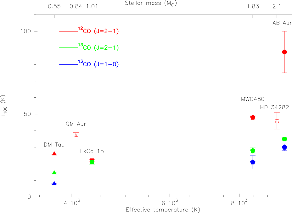
Figure 9: Temperatures derived from the CO isotopes versus effective temperature of the central star. From left to right, the sources are DM Tau (filled triangles), GM Aur (empty stars), LkCa 15 (filled squares), MWC 480 (filled pentagons), HD 34282 (empty stars) and AB Aur (filled hexagons). From top to bottom, ${}^{12}{\rm CO}$ J=2$\rightarrow$1, ${}^{13}{\rm CO}$ J=2$\rightarrow$1, ${}^{13}{\rm CO}$ J=1$\rightarrow$0 temperatures.

5.4 The LkCa 15 inner hole

In the case of LkCa 15, it is also important to mention its peculiar geometry: Piétu et al. (2006) have discovered a 50 AU cavity in the continuum emission from LkCa 15. We checked whether there is any hint of this cavity in the CO data. Adding the inner radius as an additional free parameter yields $R_{\mathrm{int}}=13\pm 5$ AU for ${}^{12}{\rm CO}$ and $R_{\mathrm{int}}=23\pm 8$ AU for ${}^{13}{\rm CO}$. These values are consistent with a smaller hole, or no hole at all, in CO and ${}^{13}{\rm CO}$. The 50 AU inner radius determined from the continuum is excluded at the 7 $\sigma$ level in ${}^{12}{\rm CO}$, and at the 3 $\sigma$ level in ${}^{13}{\rm CO}$. Moreover the fit of a hole does not significantly change the value of $p$, for both ${}^{12}{\rm CO}$ and ${}^{13}{\rm CO}$  emissions.

These small values indicate that the CO gas extends well into the continuum cavity. The cavity is thus not completely void, but still has a sufficient surface density for the ${}^{13}{\rm CO}$ lines to be detected. The LkCa 15 situation is similar to that of AB Aur, for which the apparent inner radius increases from ${}^{12}{\rm CO}$ to ${}^{13}{\rm CO}$ and to the dust emission (Piétu et al., 2005).

5.5 HCO⁺  surface density

The HCO⁺  data analysis reveal 4 major facts

• the outer radius in HCO⁺  is similar to that in ${}^{12}{\rm CO}$, and in particular it is larger than that in ${}^{13}{\rm CO}$.

• in the two cases where it could be determined, the excitation temperature of the HCO⁺ J=1$\rightarrow$0 is lower than that of the ${}^{13}{\rm CO}$ J=2$\rightarrow$1 line.

• at 300 AU, the [${}^{13}{\rm CO}$]/[HCO⁺ ] ratio is $500\pm 150$ (DM Tau), $320\pm 50$ (LkCa 15), and $1300\pm 200$ for MWC 480, with an additional uncertainty around 50 % for these last two sources due to the adopted temperature distribution. These values are similar to, although slightly smaller than the one found by Guilloteau et al. (1999) for the circumbinary disk of GG Tau ($\sim 1500$). On the other end, Pety et al. (2006) find a ratio of about 10⁴ for the low mass disk around HH 30, but at a smaller radius (100 AU).

• This ratio varies with radius: there is a tendency to have a somewhat flatter distribution of HCO⁺  than of CO (with the exception of ${}^{13}{\rm CO}$ in LkCa 15).

In DM Tau, the excitation temperature falls down to about 6 K beyond 600 AU, while the CO data indicates kinetic temperature of about 10 K in this region. Our calibration technique ensures that this is not an artifact. It may be a hint of very low temperatures in the disk mid-plane. On the other end, it may be an indication of sub-thermal excitation. However, as the critical density for the HCO⁺  J=1$\rightarrow$0  is only a few $10^{4}$ cm^-3, such a sub-thermal excitation would require that the HCO⁺  gas is located well above the disk plane. Spatially resolved observations of the HCO⁺  J=3$\rightarrow$2  transition are required to check this possibility.

5.6 Turbulence in Outer Disks

We derive intrinsic (local) line widths ranging between $0.12$ and $0.29\,{\rm km.s}^{-1}$. When taking into account the thermal component ($0.08$ to $0.15\,{\rm km.s}^{-1}$), from Eqs.6 and 7 we derive turbulent widths below 0.15 $\,{\rm km.s}^{-1}$. These values should be used as upper limits, since the spectral resolution used for the analysis (0.2 $\,{\rm km.s}^{-1}$) is comparable to the derived line widths. They are nevertheless significantly smaller than the sound speed, $C_{s}=0.3$ to $0.5\,{\rm km.s}^{-1}$ in the relevant temperature and radius range. The turbulence is thus largely subsonic. A more precise analysis, using the full spectral resolution and an accurate knowledge of the kinetic temperature distribution, is required for a better determination.

5.7 Hydrostatic Scale Height

We follow the approach which is described in Sect.3.2.5 where the scale-height is not formally derived from the hydrostatic equilibrium. In a first step, the flaring exponent $e_{h}$ is taken equal to $e_{h}=-1.25$. Such a value is in agreement with predictions from models such as Chiang & Goldreich (1997) and D’Alessio et al. (1999). The observed transitions indicate apparent scale heights at 100 AU of 30 AU in DM Tau, and 19 AU in LkCa 15 and MWC 480 (see Tab.3-5). The only discrepant result is the value derived from ${}^{12}{\rm CO}$ in MWC 480, 10 AU. In a second step, treating $e_{h}$ as a free parameter provides similar results, except for LkCa 15 where the ${}^{13}{\rm CO}$ data is best fitted by a flat ($e_{h}=0$), but thick disk (see Fig.5).

On the other end, using the temperature derived from the ${}^{13}{\rm CO}$ J=2$\rightarrow$1  transition as appropriate, we can derive the hydrostatic scales heights. These scale heights are 15, 13 and 9.5 AU, respectively for DM Tau, LkCa 15 and MWC 480, with a typical exponent $e_{h}=-1.35$, approximately 1.5 – 2 times smaller than the apparent values. Although, as mentioned in Sect.3.2.5, the scale height has to be interpreted with some caution (especially when determined from ${}^{12}{\rm CO}$), these results suggest that CO has a broader vertical distribution than what is expected from an hydrostatic distribution of the gas. The current data do not allow us to identify the causes of this effect. Vertical spreading due to turbulence can be rejected as the turbulence is largely subsonic (see Sect.5.6). The larger apparent height may be due to CO being more abundant in the photo-dissociation layer above the disk plane.

5.8 Comparison with other Disks and Models

Only one other source has been studied at the same level in the CO isotopologues: AB Aur by Piétu et al. (2005). The temperature behavior of the AB Aur disk is similar to that of the MWC 480 disk, although the AB Aur disk is warmer. Temperature derived from CO for all sources are summarized in Fig.9. As expected, the disk temperatures (midplane and surface) clearly increase with the stellar luminosity. The A0/A1 star HD34282, mapped by Piétu et al. (2003) in ${}^{12}{\rm CO}$  also exhibits a hotter disk surface while the TTauri star GM Aur (Dutrey et al., 1998) has a colder disk. From Table 1 of Piétu et al. (2005), the ${}^{13}{\rm CO}$ surface density in AB Aur at 300 AU is about $2\,10^{16}$ cm^-2, 4 to 8 times larger than in the DM Tau, MWC 480 or LkCa 15 disks. This larger surface density probably results from a lack of depletion onto dust grains, since the temperature in the AB Aur disk remains well above the CO condensation temperature at least up to 700 AU in radius, contrary to those of DM Tau, LkCa 15 and MWC 480 which are much colder beyond 200 - 300 AU.

LkCa 15 differs slightly from the general picture: no clear vertical temperature gradient is observed, and the ${}^{13}{\rm CO}$ surface density slope is much less steep (exponent $p=1.5$) and the CO isotopologues indicate a discrepant scale height behaviour. This may be linked to a peculiar disk geometry: Piétu et al. (2006) have reported a 50 AU cavity in the continuum emission from LkCa 15, perhaps due to planetary formation or a low mass companion. This peculiar geometry may affect the temperature structure of the surrounding disk, by for example shielding it from stellar radiation behind a warm, thick, inner rim. Any definite conclusion about the peculiarities of LkCa 15 seems premature at this point.

Molecular abundances in proto-planetary disks have been studied by several authors. Disks are believed to be dominated by a warm molecular layer, exposed to the UV radiation emanating from the central star. van Zadelhoff et al. (2003) showed 2-D radiative transfer effects result in a stronger penetration of the UV field into the disk than simple 1+1D models assumed. A more refined model was published by Aikawa & Nomura (2006), which use a time dependent chemistry taking into account the thermal structure of the disk, 2-D radiative transfer and sticking onto grains. Their model parameters are more appropriate for DM Tau. Despite its comprehensiveness, this model fails to represent the observed surface densities: it predicts relatively shallow ($p\simeq 1$) radial distribution of the surface density, in sharp contrast with the steep slope observed. However, their model only extends out to 300 AU, while the constraint we obtain on the surface densities in DM Tau refer mostly to larger radii.

Semenov et al. (2006) point out the importance of vertical mixing in explaining the molecular surface densities. A similar study was conducted by Willacy et al. (2006) who conclude that a diffusion coefficient of order 10¹⁸ cm²s^-1 is required to bring the CO surface density in reasonable agreement with observations. Vertical mixing may be essential in explaining why CO is detected at temperature well below the freeze out value, and also why, despite very different temperature profiles, DM Tau and MWC 480 display similar CO surface densities.

None of these model studied the ${}^{13}{\rm CO}$  isotopologue. Hily-Blant et al. (2007) used a simpler PDR model to study the effects of grain size and stellar UV flux on the CO isotopologue abundances. In this static model, self-shielding of H₂, CO and ${}^{13}{\rm CO}$ is treated explicitly, but CO sticking onto grains is not included. This model shows the importance of fractionation and reproduces better the observed surface densities. In particular, from their Fig.6, [${}^{12}{\rm CO}$]/[${}^{13}{\rm CO}$] ratio of order 10 – 20 is obtained for large grains ($a_{+}=3\,10^{-4}$ m) and $\chi=1000$ ($\chi$ being the enhancement over the interstellar UV field at 100 AU, with a 1/r² dependence), i.e. when the UV field penetration is important.

So far, no published model reproduces the smaller outer radii for ${}^{13}{\rm CO}$ than for ${}^{12}{\rm CO}$. To do so, it seems essential to account for selective photodissociation of CO isotopologues by the interstellar UV radiation field, and in particular by the UV radiation impinging on the disk outer edge. The disappearance of ${}^{13}{\rm CO}$ at distances $\sim 500$ AU from MWC 480 and LkCa 15 indicate that the typical extinction through the disk at this radius corresponds roughly to $A_{V}\simeq 1$, although the disks extend at least to 700 - 900 AU. A consistency check can be done on this hypothesis: assuming a standard $A_{V}/$H₂ ratio, the ${}^{13}{\rm CO}$ outer radius can be used to constrain the CO abundance at this distance. From Fig.4-6, the typical ${}^{12}{\rm CO}$ surface density at the ${}^{13}{\rm CO}$ outer radius is $2-4\,10^{15}$ cm^-2, which converts to X[${}^{12}{\rm CO}$] $\simeq 3-6\,10^{-5}$, in good agreement with the expectation in this transition region. In DM Tau, $A_{V}\simeq 1$ would occur near 800 AU, i.e. the (outer) DM Tau disk is more opaque than those of MWC 480 and LkCa 15. This larger opacity can result either from a larger H₂ density, or from a larger $A_{V}/$H₂, i.e. more small grains in DM Tau.

All the chemical models are hampered by the need to specify the appropriate H₂ density distribution and the dust properties. These parameters remain largely unknown. The values of $p$ and $R_{\mathrm{out}}$ for the dust in LkCa 15 and MWC 480 derived by Piétu et al. (2006) differ systematically from those found here for CO. In addition, the absolute value of the absorption coefficient of dust is also uncertain, which makes the derivation of an H₂ surface density through continuum observations quite difficult. Using the parameters given by Piétu et al. (2006), we find at the dust core outer radius, $\approx 180$ AU, that the CO abundance is $\sim 10^{-6}$ for LkCa 15, while it is $\sim 3\,10^{-7}$– $3\,10^{-6}$ for MWC 480, depending on which temperature profile is adopted for the dust. These very low values, as well as the very different values of the exponent $p$ for dust and CO, may thus indicate that the H₂ surface density cannot be extrapolated by a simple power law, but displays instead a very significant change near $\sim 150$ AU. This can have significant impact on the chemical model predictions for any specific disk.

6 Summary

We report new ${}^{13}{\rm CO}$  observations in LkCa 15 and MWC 480 obtained with the IRAM array, and HCO⁺   observations of LkCa 15 and MWC 480 and DM Tau. These data were analyzed together with existing ${}^{12}{\rm CO}$  data. As we improved our modelling method, we also carried again the analysis on DM Tau data as a consistency check. By comparing these results with previous one obtained on AB Aur (and to the temperatures derived from ${}^{12}{\rm CO}$ observations in HD34282 and GM Aur), this allowed us to derive the following conclusions:

• We systematically detect radial gas temperature gradients. Vertical temperature gradients are also ubiquitous in AB Aur, DM Tau, and MWC 480, but LkCa 15 is an apparent exception (perhaps due to its peculiar geometry). Disks surrounding hotter stars, such as Herbig Ae objects (MWC 480 and AB Aur), present a hotter CO surface. This behavior agrees with the prediction from models of passive irradiated disks.

• CO disks around hotter stars are also hotter around the mid-plane (AB Aur and to a lesser extent MWC 480). Although [CO/H₂] ratios are not directly measurable, the much higher surface density of ${}^{13}{\rm CO}$ in the warmest disk, AB Aur, indicates that depletion onto grains is an important mechanism for the colder disks. However, the CO surface density does not appear to be a monotonous function of the stellar type.

• For the more sensitive transitions, we are able to measure an apparent scale height which appears to be larger than the hydrostatic scale height. Although marginal, this result is in agreement with the expectation that molecules preferentially form in a warm photo-dissociation layer above the disk plane.

• However, in the outer part of TTauri disks ($R\geq 300$ AU) and even around MWC 480, the averaged kinetic temperature measured along the line of sight is well below the freeze-out temperature of CO, but a significant amount of CO is still observed. This is in contradiction with most predictions of chemical models but would be in favor of models with vertical mixing.

• The CO surface density falls off much more rapidly with radius than predicted by most chemical models. In the cases of DM Tau and LkCa 15, we also observe that the ${}^{12}{\rm CO}$  has a steeper surface density exponent than ${}^{13}{\rm CO}$. This suggests a steepening of the surface density slope beyond 300 – 500 AU, but photo-dissociation, and also perhaps depletion on grains are likely to play a role.

• A change in surface density behaviour is also suggested by the very different parameters (exponent $p$ and outer radius) derived from the continuum emission.

• For all disks where ${}^{12}{\rm CO}$ and ${}^{13}{\rm CO}$ data are available, photo-dissociation by the ambient UV field impinging on the disk edge is likely the appropriate mechanism to explain the smaller outer radii determined in ${}^{13}{\rm CO}$ compared to that of ${}^{12}{\rm CO}$.

• Except for the warmest disks, CO fractionation is an important mechanism. For DM Tau and LkCa 15, we estimate an isotopologue ratio, of order or less than 10 – 20 between 300 AU and the ${}^{13}{\rm CO}$ outer radius.

• At 300 AU, the [${}^{13}{\rm CO}$]/[HCO⁺ ] ratio is around 600, within a factor 2. It apparently decreases with radius.