Dissipationless collapses in MOND

Abstract

Dissipationless collapses in Modified Newtonian Dynamics (MOND) are studied by using a new particle-mesh N-body code based on our numerical MOND potential solver. We found that low surface-density end-products have shallower inner density profile, flatter radial velocity-dispersion profile, and more radially anisotropic orbital distribution than high surface-density end-products. The projected density profiles of the final virialized systems are well described by Sersic profiles with index $m{\,\mathrel{\mathchoice{\lower 2.9pt\vbox{\halign{$\m@th\displaystyle\hfil#\hfil$\cr<\crcr\sim\crcr}}}{\lower 2.9pt\vbox{\halign{$\m@th\textstyle\hfil#\hfil$\cr<\crcr\sim\crcr}}}{\lower 2.9pt\vbox{\halign{$\m@th\scriptstyle\hfil#\hfil$\cr<\crcr\sim\crcr}}}{\lower 2.9pt\vbox{\halign{$\m@th\scriptscriptstyle\hfil#\hfil$\cr<\crcr\sim\crcr}}}\,}}4$, down to $m\sim 2$ for a deep-MOND collapse. Consistently with observations of elliptical galaxies, the MOND end-products, if interpreted in the context of Newtonian gravity, would appear to have little or no dark matter within the effective radius. However, we found impossible (under the assumption of constant mass-to-light ratio) to simultaneously place the resulting systems on the observed Kormendy, Faber-Jackson and Fundamental Plane relations of elliptical galaxies. Finally, the simulations provide strong evidence that phase mixing is less effective in MOND than in Newtonian gravity.

1. Introduction

In Bekenstein & Milgrom’s (1984, hereafter BM) Lagrangian formulation of Milgrom’s (1983) Modified Newtonian Dynamics (MOND), the Poisson equation

$$\nabla^{2}\phi_{\rm N}=4\pi G\rho$$ (1)

for the Newtonian gravitational potential $\phi_{\rm N}$ is replaced by the field equation

$$\nabla\cdot\left[\mu\left({\|\nabla\phi\|\over a_{0}}\right)\nabla\phi\right]=4\pi G\rho,$$ (2)

where $a_{0}\simeq 1.2\times 10^{-10}{\rm m\,s^{-2}}$ is a characteristic acceleration, $\|...\|$ is the standard Euclidean norm, $\phi$ is the MOND gravitational potential produced by the density distribution $\rho$, and in finite mass systems $\nabla\phi\to 0$ for $\|{\bf x}\|\to\infty$. The MOND gravitational field ${\bf g}$ experienced by a test particle is

$${\bf g}=-\nabla\phi,$$ (3)

and the function $\mu$ is such that

$$\mu(y)\sim\cases{y&for $y\ll 1$,\cr 1&for $y\gg 1$;}$$ (4)

throughout this paper we use

$$\mu(y)={y\over\sqrt{1+y^{2}}}.$$ (5)

In the so-called ‘deep MOND regime’ (hereafter dMOND), describing low-acceleration systems ($\|\nabla\phi\|\ll a_{0}$), $\mu(y)=y$ and so equation (2) simplifies to

$$\nabla\cdot\left({\|\nabla\phi\|}\nabla\phi\right)=4\pi Ga_{0}\rho.$$ (6)

The source term in equation (2) can be eliminated by using equation (1), giving

$$\mu\left(\|\nabla\phi\|\over a_{0}\right)\nabla\phi=\nabla\phi_{\rm N}+{\bf S},$$ (7)

where ${\bf S}={\rm curl\,}{\bf h}$ is a solenoidal field dependent on $\rho$ and in general different from zero. When ${\bf S}=0$ equation (7) reduces to Milgrom’s (1983) formulation and can be solved explicitly. Such reduction is possible for configurations with spherical, cylindrical or planar symmetry, which are special cases of a more general family of stratifications (BM; Brada & Milgrom 1995). Though the solenoidal field ${\bf S}$ has been shown to be small for some configurations (Brada & Milgrom 1995; Ciotti, Londrillo & Nipoti 2006, hereafter CLN), neglecting it when simulating time-dependent dynamical processes has dramatic effects such as non-conservation of total linear momentum (e.g. Felten 1984; see also Section 3.1).

Nowadays several astronomical observational data appear consistent with the MOND hypothesis (see, e.g., Milgrom 2002; Sanders & McGaugh 2002). In addition, Bekenstein (2004) recently proposed a relativistic version of MOND (Tensor-Vector-Scalar theory, TeVeS), making it an interesting alternative to the cold dark matter paradigm. However, dynamical processes in MOND have been investigated very little so far, mainly due to difficulties posed by the non-linearity of equation (2). Here we recall the spherically symmetric simulations (in which ${\bf S}=0$) of gaseous collapse in MOND by Stachniewicz & Kutschera (2005) and Nusser & Pointecouteau (2006). The only genuine three-dimensional MOND N-body simulations (in which equation [2] is solved exactly) are those by Brada & Milgrom (1999, 2000), who studied the stability of disk galaxies and the external field effect, and those of Tiret & Combes (2007). Other attempts to study MOND dynamical processes have been conducted using three-dimensional N-body codes by arbitrarily setting ${\bf S}=0$: Christodoulou (1991) investigated disk stability, while Nusser (2002) and Knebe & Gibson (2004) explored cosmological structure formation.

In this paper we present results of N-body simulations of dissipationless collapse in MOND. The simulations were performed with an original three-dimensional particle-mesh N-body code, based on the numerical MOND potential solver presented in CLN, which solves equation (2) exactly. These numerical experiments are interesting both from a purely dynamical point of view, allowing for the first time to explore the relaxation processes in MOND, and in the context of elliptical galaxy formation. In fact, the ability of dissipationless collapse at producing systems strikingly similar to real ellipticals is a remarkable success of Newtonian dynamics (e.g., van Albada 1982; Aguilar & Merritt 1990; Londrillo, Messina & Stiavelli 1991; Udry 1993; Trenti, Bertin & van Albada 2005; Nipoti, Londrillo, & Ciotti 2006, hereafter NLC06), while there have been no indications so far that MOND can work as well in this respect. Here we study the structural and kinematical properties of the end-products of MOND simulations, and we compare them with the observed scaling relations of elliptical galaxies: the Faber–Jackson (FJ) relation (Faber & Jackson 1976), the Kormendy (1977) relation, and the Fundamental Plane (FP) relation (Djorgovski & Davis 1987, Dressler et al. 1987).

The paper is organized as follows. The main features of the new N-body code are presented in Section 2, while Section 3 describes the set-up and the analysis of the numerical simulations. The results are presented in Section 4 and discussed in Section 5.

2. The N-body code

While most N-body codes for simulations in Newtonian gravity are based on the gridless multipole expansion treecode scheme (Barnes & Hut 1986; see also Dehnen 2002), the non-linearity of the MOND field equation (2) forces one to resort to other methods, such as the particle-mesh technique (see Hockney & Eastwood 1988). In this approach, particles are moved under the action of a gravitational field which is computed on a grid, with particle-mesh interpolation providing the link between the two representations. In our MOND particle-mesh N-body code, we adopt a spherical grid of coordinates ($r$, $\vartheta$, $\varphi$), made of $N_{r}\times N_{\vartheta}\times N_{\varphi}$ points, on which the MOND field equation is solved as in CLN. Particle-mesh interpolations are obtained with a quadratic spline in each coordinate, while time stepping is given by a classical leap-frog scheme (Hockney & Eastwood 1988). The time-step $\Delta t$ is the same for all particles and is allowed to vary adaptively in time. In particular, according to the stability criterion for the leap-frog time integration, we adopt $\Delta t=\eta/\sqrt{\max{|\nabla^{2}\phi|}}$, where $\eta{\,\mathrel{\mathchoice{\lower 2.9pt\vbox{\halign{$\m@th\displaystyle\hfil#\hfil$\cr<\crcr\sim\crcr}}}{\lower 2.9pt\vbox{\halign{$\m@th\textstyle\hfil#\hfil$\cr<\crcr\sim\crcr}}}{\lower 2.9pt\vbox{\halign{$\m@th\scriptstyle\hfil#\hfil$\cr<\crcr\sim\crcr}}}{\lower 2.9pt\vbox{\halign{$\m@th\scriptscriptstyle\hfil#\hfil$\cr<\crcr\sim\crcr}}}\,}}0.3$ is a dimensionless parameter. We found that $\eta=0.1$ assures good conservation of the total energy in the Newtonian cases (see Section 3.1). In the present version of the code, all the computations on the particles and the particle-mesh interpolations can be split among different processors, while the computations relative to the potential solver are not performed in parallel. The solution of equation (2) over the grid is then the bottleneck of the simulations: however, the iterative procedure on which the potential solver is based (see CLN) allows to adopt as seed solution at each time step the potential previously determined.

The MOND potential solver can also solve the Poisson equation (obtained by imposing $\mu=1$ in equation 2), so Newtonian simulations can be run with the same code. We exploited this property to test the code by running several Newtonian simulations of both equilibrium distributions and collapses, comparing the results with those of simulations (starting from the same initial conditions) performed with the FVFPS treecode (Londrillo, Nipoti & Ciotti 2003; Nipoti, Londrillo & Ciotti 2003). One of these tests is described in Section 4.1.2.

We also verified that the code reproduces the Newtonian and MOND conservation laws (see Section 3.1): note that the conservation laws in MOND present some peculiarities with respect to the Newtonian case, so we give here a brief discussion of the subject. As already stressed by BM, equation (2) is obtained from a variational principle applied to a Lagrangian with all the required symmetries, so energy, linear and angular momentum are conserved. Unfortunately, as also shown by BM, the total energy diverges even for finite mass systems, thus posing a computational challenge to code validation. We solved this problem by checking the volume-limited energy balance equation

$${d\over dt}\int_{V_{0}}\left[k+\rho\phi+{a_{0}^{2}\over 8\pi G}\mathcal{F}\left({||\nabla\phi||\over a_{0}}\right)\right]d^{3}{\bf x}=$$

$${1\over 4\pi G}\int_{\partial V_{0}}\mu{\partial\phi\over\partial t}<\nabla\phi,\hat{\bf n}>da,$$ (8)

which is derived in Appendix A. In equation (2) $V_{0}$ is an arbitrary (but fixed) volume enclosing all the system mass, $k$ is the kinetic energy per unit volume, and

$$\mathcal{F}(y)\equiv 2\int_{y_{0}}^{y}\mu(\xi)\xi d\xi,$$ (9)

where $y_{0}$ is an arbitrary constant; note that only finite quantities are involved. Another important relation between global quantities for a system at equilibrium (in MOND as in Newtonian gravity) is the virial theorem

$$2K+W=0,$$ (10)

where $K$ is the total kinetic energy and $W={\rm Tr}\,W_{ij}$ is the trace of the Chandrasekhar potential energy tensor

$$W_{ij}\equiv-\int\rho({\bf x})x_{i}{\partial\phi({\bf x})\over\partial x_{j}}d^{3}{\bf x}$$ (11)

(e.g., Binney & Tremaine 1987). Note that in MOND $K+W$ is not the total energy, and is not conserved. However, $W$ is conserved in the limit of dMOND, being $W=-(2/3)\sqrt{Ga_{0}M_{*}^{3}}$ for all systems of finite total mass ${M_{*}}$ (see Appendix B for the proof). As a consequence, in dMOND the virial theorem writes simply $\sigma_{\rm V}^{4}=4G{M_{*}}a_{0}/9$, where $\sigma_{\rm V}\equiv\sqrt{2K/{M_{*}}}$ is the system virial velocity dispersion (this relation was proved for dMOND spherical systems by Gerhard & Spergel 1992; see also Milgrom 1984). In our simulations we also tested that equation (10) is satisfied at equilibrium, and that $W$ is conserved in the dMOND case (see Sections 3.1 and 4).

3. Numerical simulations

Table 1Time, velocity, and energy units for Newtonian and MOND (subscript n), and dMOND (subscript d) N-body simulations.

$t_{\rm*n}=r_{*}^{3/2}(G{M_{*}})^{-1/2}$	$t_{\rm*d}=r_{*}(G{M_{*}}a_{0})^{-1/4}$
$v_{\rm*n}=(G{M_{*}})^{1/2}r_{*}^{-1/2}$	$v_{\rm*d}=(G{M_{*}}a_{0})^{1/4}$
$E_{\rm*n}=G{M_{*}}^{2}r_{*}^{-1}$	$E_{\rm*d}=(Ga_{0})^{1/2}{M_{*}}^{3/2}$

The choice of appropriate scaling physical units is an important aspect of N-body simulations. This is especially true in the present case, in which we want to compare MOND and Newtonian simulations having the same initial conditions. As well known, due to the scale-free nature of Newtonian gravity, a Newtonian $N$-body simulation starting from a given initial condition describes in practice $\infty^{2}$ systems of arbitrary mass and size. Each of them is obtained by assigning specific values to the length and mass units, $r_{*}$ and ${M_{*}}$, in which the initial conditions are expressed. Also dMOND gravity is scale free, because $a_{0}$ appears only as a multiplicative factor in equation (6), and so a simulation in dMOND gravity represents systems with arbitrary mass and size (though in principle the results apply only to systems with accelerations much smaller than $a_{0}$). MOND simulations can also be rescaled, but, due to the presence of the characteristic acceleration $a_{0}$ in the non-linear function $\mu$, each simulation describes only $\infty^{1}$ systems, because $r_{*}$ and ${M_{*}}$ cannot be chosen independently of each other.

On the basis of the above discussion, we fix the physical units as follows (see Appendix C for a detailed description of the scaling procedure). Let the initial density distribution be characterized by a total mass ${M_{*}}$ and a characteristic radius $r_{*}$. We rescale the field equations so that the dimensionless source term is the same in Newtonian, MOND and dMOND simulations. We also require that the Second Law of Dynamics, when cast in dimensionless form, is independent of the specific force law considered, and this leads to fix the time unit. As a result, Newtonian and MOND simulations have the same time unit $t_{\rm*n}=r_{*}^{3/2}(G{M_{*}})^{-1/2}$, while the natural time unit in dMOND simulations is $t_{\rm*d}=r_{*}(G{M_{*}}a_{0})^{-1/4}$. Note that MOND simulations are characterized by the dimensionless parameter $\kappa=G{M_{*}}/r_{*}^{2}a_{0}$, and scaling of a specific simulation is allowed provided the value of $\kappa$ is maintained constant. So, simulations with lower $\kappa$ values describe lower surface-density, weaker acceleration systems; dMOND simulations represent the limit case $\kappa\ll 1$, while Newtonian ones describe the regime with $\kappa\gg 1$. With the time units fixed, the corresponding velocity and energy units are $v_{\rm*n}\equiv r_{*}/t_{\rm*n}$, $v_{\rm*d}\equiv r_{*}/t_{\rm*d}$, $E_{\rm*n}={M_{*}}v_{\rm*n}^{2}$, and $E_{\rm*d}={M_{*}}v_{\rm*d}^{2}$ (see Table 1 for a summary).

Figure 1.— Time evolution of $2K/|W|$, $K$, $W$, and $K+W$ for simulations D, M1, and N. $K$, $W$, and $K+W$ are in units of $E_{\rm*d}$ (left column), and $E_{\rm*n}$ (central and right columns). For clarity, the time axes are zoomed-in between 0 and 10.

3.1. Initial conditions and analysis of the simulations

We performed a set of five dissipationless-collapse N-body simulations, starting from the same phase-space configuration: the initial particle distribution follows the Plummer (1911) spherically symmetric density distribution

$$\rho(r)={{3{M_{*}}r_{*}^{2}}\over 4{\pi(r^{2}+r_{*}^{2})^{5/2}}},$$ (12)

where ${M_{*}}$ is the total mass and $r_{*}$ a characteristic radius. The choice of a Plummer sphere as initial condition is quite artificial, and not necessarily the most realistic to reproduce initial conditions in the cosmological context (e.g., Gunn & Gott 1972). We adopt such a distribution to adhere to other papers dealing with collisionless collapse (e.g., Londrillo et al. 1991; NLC06; see also Section 5, in which we present the results of a set of simulations starting from different initial conditions). The particles are at rest, so the initial virial ratio $2K/|W|=0$. What is different in each simulation is the adopted gravitational potential, which is Newtonian in simulation N, dMOND in simulation D, and MOND with acceleration ratio $\kappa$ in simulations M$\kappa$ ($\kappa$=1, 2, 4). For each simulation we define the dynamical time $t_{\rm dyn}$ as the time at which the virial ratio $2K/|W|$ reaches its maximum value. In particular, we find $t_{\rm dyn}\sim 2t_{\rm*d}$ in simulation D, and $t_{\rm dyn}\sim 2t_{\rm*n}$ in simulations N, M1, M2 and M4. We note that $t_{\rm dyn}\sim{G{M_{*}}^{5/2}(2|K+W|)^{-3/2}}$ in simulation N.

Following NLC06, the particles are spatially distributed according to equation (12) and then randomly shifted in position (up to $r_{*}/5$ in modulus). This artificial, small-scale ”noise” is introduced to enhance the phase mixing at the beginning of the collapse, because the numerical noise is small, and the velocity dispersion is zero (see also Section 4.2). As such, these fluctuations are not intended to reproduce any physical clumpiness.

All the simulations (realized with $N=10^{6}$ particles, and a grid with $N_{r}=64$, $N_{\vartheta}=16$ and $N_{\varphi}=32$) are evolved up $t=150t_{\rm dyn}$. In all cases the modulus of the center of mass position oscillates around zero with r.m.s ${\,\mathrel{\mathchoice{\lower 2.9pt\vbox{\halign{$\m@th\displaystyle\hfil#\hfil$\cr<\crcr\sim\crcr}}}{\lower 2.9pt\vbox{\halign{$\m@th\textstyle\hfil#\hfil$\cr<\crcr\sim\crcr}}}{\lower 2.9pt\vbox{\halign{$\m@th\scriptstyle\hfil#\hfil$\cr<\crcr\sim\crcr}}}{\lower 2.9pt\vbox{\halign{$\m@th\scriptscriptstyle\hfil#\hfil$\cr<\crcr\sim\crcr}}}\,}}0.1r_{*}$; similarly, the modulus of the total angular momentum oscillates around zero with r.m.s. ${\,\mathrel{\mathchoice{\lower 2.9pt\vbox{\halign{$\m@th\displaystyle\hfil#\hfil$\cr<\crcr\sim\crcr}}}{\lower 2.9pt\vbox{\halign{$\m@th\textstyle\hfil#\hfil$\cr<\crcr\sim\crcr}}}{\lower 2.9pt\vbox{\halign{$\m@th\scriptstyle\hfil#\hfil$\cr<\crcr\sim\crcr}}}{\lower 2.9pt\vbox{\halign{$\m@th\scriptscriptstyle\hfil#\hfil$\cr<\crcr\sim\crcr}}}\,}}0.02$, in units of $r_{*}{M_{*}}v_{\rm*n}$ (simulations M$\kappa$ and N) and of $r_{*}{M_{*}}v_{\rm*d}$ (simulation D). $K+W$ in the Newtonian simulation and $W$ in the dMOND simulation are conserved to within $2\%$ and $0.6\%$, respectively. The volume-limited energy balance equation (2) is conserved with an accuracy of $1\%$ in MOND simulations, independently of the adopted $V_{0}$. To estimate possible numerical effects, we reran one of the MOND collapse simulations (M1) using $N=2\times 10^{6}$, $N_{r}=80$, $N_{\vartheta}=24$, and $N_{\varphi}=48$: we found that the end-products of these two simulations do not differ significantly, as far as the properties relevant to the present work are concerned.

The intrinsic and projected properties of the collapse end-products are determined as in NLC06. In particular, the position of the center of the system is determined using the iterative technique described by Power et al. (2003). Following Nipoti et al. (2002), we measure the axis ratios $c/a$ and $b/a$ of the inertia ellipsoid (where $a$, $b$ and $c$ are the major, intermediate and minor axis) of the final density distributions, their angle-averaged profile and half-mass radius $r_{\rm h}$. We fitted the final angle-averaged density profiles with the $\gamma$-model (Dehnen 1993; Tremaine et al. 1994)

$$\rho(r)={\rho_{0}r_{\rm c}^{4}\over r^{\gamma}(r_{\rm c}+r)^{4-\gamma}},$$ (13)

where the inner slope $\gamma$ and the break radius $r_{\rm c}$ are free parameters, and the reference density $\rho_{0}$ is fixed by the total mass ${M_{*}}$. The fitting radial range is $0.06\,{\,\mathrel{\mathchoice{\lower 2.9pt\vbox{\halign{$\m@th\displaystyle\hfil#\hfil$\cr<\crcr\sim\crcr}}}{\lower 2.9pt\vbox{\halign{$\m@th\textstyle\hfil#\hfil$\cr<\crcr\sim\crcr}}}{\lower 2.9pt\vbox{\halign{$\m@th\scriptstyle\hfil#\hfil$\cr<\crcr\sim\crcr}}}{\lower 2.9pt\vbox{\halign{$\m@th\scriptscriptstyle\hfil#\hfil$\cr<\crcr\sim\crcr}}}\,}}\,r/r_{\rm h}\,{\,\mathrel{\mathchoice{\lower 2.9pt\vbox{\halign{$\m@th\displaystyle\hfil#\hfil$\cr<\crcr\sim\crcr}}}{\lower 2.9pt\vbox{\halign{$\m@th\textstyle\hfil#\hfil$\cr<\crcr\sim\crcr}}}{\lower 2.9pt\vbox{\halign{$\m@th\scriptstyle\hfil#\hfil$\cr<\crcr\sim\crcr}}}{\lower 2.9pt\vbox{\halign{$\m@th\scriptscriptstyle\hfil#\hfil$\cr<\crcr\sim\crcr}}}\,}}\,10$. In order to estimate the importance of projection effects, for each end-product we consider three orthogonal projections along the principal axes of the inertia tensor, measuring the ellipticity $\epsilon=1-b_{\rm e}/a_{\rm e}$, the circularized projected density profile and the circularized effective radius $R_{\rm e}\equiv\sqrt{a_{\rm e}b_{\rm e}}$ (where $a_{\rm e}$ and $b_{\rm e}$ are the major and minor semi-axis of the effective isodensity ellipse). We fit (over the radial range $0.1\,{\,\mathrel{\mathchoice{\lower 2.9pt\vbox{\halign{$\m@th\displaystyle\hfil#\hfil$\cr<\crcr\sim\crcr}}}{\lower 2.9pt\vbox{\halign{$\m@th\textstyle\hfil#\hfil$\cr<\crcr\sim\crcr}}}{\lower 2.9pt\vbox{\halign{$\m@th\scriptstyle\hfil#\hfil$\cr<\crcr\sim\crcr}}}{\lower 2.9pt\vbox{\halign{$\m@th\scriptscriptstyle\hfil#\hfil$\cr<\crcr\sim\crcr}}}\,}}\,R/R_{\rm e}\,{\,\mathrel{\mathchoice{\lower 2.9pt\vbox{\halign{$\m@th\displaystyle\hfil#\hfil$\cr<\crcr\sim\crcr}}}{\lower 2.9pt\vbox{\halign{$\m@th\textstyle\hfil#\hfil$\cr<\crcr\sim\crcr}}}{\lower 2.9pt\vbox{\halign{$\m@th\scriptstyle\hfil#\hfil$\cr<\crcr\sim\crcr}}}{\lower 2.9pt\vbox{\halign{$\m@th\scriptscriptstyle\hfil#\hfil$\cr<\crcr\sim\crcr}}}\,}}\,10$) the circularized projected density profiles of the end-products with the $R^{1/m}$ Sersic (1968) law:

$$I(R)=I_{\rm e}\,\exp\left\{-b(m)\left[\left(\frac{R}{R_{\rm e}}\right)^{1/m}-1\right]\right\},$$ (14)

where $I_{\rm e}\equiv I(R_{\rm e})$ and $b(m)\simeq 2m-1/3+4/405m$ (Ciotti & Bertin 1999). In the fitting procedure $m$ is the only free parameter, because $R_{\rm e}$ and $I_{\rm e}$ are determined by their measured values obtained by particle count. In addition, we measure the central velocity dispersion $\sigma_{0}$, obtained by averaging the projected velocity dispersion over the circularized surface density profile within an aperture of $R_{\rm e}/8$. Some of these structural parameters are reported in Table 2 for the five simulations described above, as well as for three additional simulations, which start from different initial conditions (see Section 5).

4. Results

In Newtonian gravity, collisionless systems reach virialization through violent relaxation in few dynamical times, as predicted by the theory (Lynden-Bell 1967) and confirmed by numerical simulations (e.g. van Albada 1982). On the other hand, due to the non linearity of the theory and the lack of numerical simulations, the details of relaxation processes and virialization in MOND are much less known. Thus, before discussing the specific properties of the collapse end-products we present a general overview of the time evolution of the virial quantities in our simulations, postponing to Section 4.2 a more detailed description of the phase-space evolution. In particular, in Fig. 1 we show the time evolution of $2K/|W|$, $K$, $W$, and $K+W$ for simulations D, M1, and N. In the diagrams time is normalized to $t_{\rm dyn}$, so plots referring to different simulations are directly comparable (the values of $t_{\rm dyn}$ in time units for the five simulations are given in Section 3.1). In simulation N (right column) we find the well known behavior of Newtonian dissipationless collapses: $2K/|W|$ has a peak, then oscillates, and eventually converges to the equilibrium value $2K/|W|=1$; the total energy $K+W$ is nicely conserved during the collapse, though it presents a secular drift, a well known feature of time integration in N-body codes. The time evolution of the same quantities is significantly different in a dMOND simulation (left column). In particular, the virial ratio $2K/|W|$ quickly becomes close to one, but is still oscillating at very late times because of the oscillations of $K$, while $W$ is constant as expected. As we show in Section 4.2, these oscillations are related to a peculiar behavior of the system in phase space. Finally, simulation M1 (central column) represents an intermediate case between models N and D: the system starts as dMOND, but soon its core becomes concentrated enough to enter the Newtonian regime. After the initial phases of the collapse, Newtonian gravity acts effectively in damping the oscillations of the virial ratio. Overall, it is apparent how the system is in a “mixed” state, neither Newtonian ($K+W$ is not conserved) nor dMOND ($W$ is not constant).

4.1. Properties of the collapse end-products

4.1.1 Spatial and projected density profiles

Figure 2.— Angle-averaged density, radial velocity-dispersion and anisotropy-parameter profiles (from bottom to top) for the end-products of simulations D, M1, and N. Dotted lines in the bottom panels represent $\rho\propto r^{-1}$ profiles, which are shown for reference. Empty circles in the right column show the corresponding profiles obtained with the FVFPS treecode from the same initial conditions.

Figure 3.— Line-of-sight velocity-dispersion profiles (top), circularized projected density profiles and residuals of the Sersic fit (bottom) of the end-products of simulations D, M1, and N (squares; 1-$\sigma$ error bars are always smaller than the symbol size). The dotted lines are the best-fitting Sersic models.

We found that all the simulated systems, once virialized, are not spherically symmetric. However, while the dMOND collapse end-product is triaxial ($c/a\sim 0.2$, $b/a\sim 0.4$), MOND and Newtonian end-products are oblate ($c/a\sim c/b\sim 0.5$). The ellipticity $\epsilon$ of the projected density distributions (measured for each of the principal projections) is found in the range $0.5-0.8$ in D, and $0-0.5$ in M1, M2, M4 and N. These values are consistent with those observed in real ellipticals, with the exception of $\epsilon_{b}$ in model D (see Table 2), which would correspond - if taken at face value - to an E8 galaxy. These result could be just due to the procedure adopted to measure the ellipticity (see Section 3.1), however we find interesting that dMOND gravity could be able to produce some system that would be unstable in Newtonian gravity. We remark that a similar result, in the different context of disk stability in MOND, has been obtained by Brada & Milgrom (1999).

In order to describe the radial mass distribution of the final virialized systems, we fitted their angle-averaged density profiles with the $\gamma$-model (13) over the radial range $0.06\,{\,\mathrel{\mathchoice{\lower 2.9pt\vbox{\halign{$\m@th\displaystyle\hfil#\hfil$\cr<\crcr\sim\crcr}}}{\lower 2.9pt\vbox{\halign{$\m@th\textstyle\hfil#\hfil$\cr<\crcr\sim\crcr}}}{\lower 2.9pt\vbox{\halign{$\m@th\scriptstyle\hfil#\hfil$\cr<\crcr\sim\crcr}}}{\lower 2.9pt\vbox{\halign{$\m@th\scriptscriptstyle\hfil#\hfil$\cr<\crcr\sim\crcr}}}\,}}\,r/r_{\rm h}\,{\,\mathrel{\mathchoice{\lower 2.9pt\vbox{\halign{$\m@th\displaystyle\hfil#\hfil$\cr<\crcr\sim\crcr}}}{\lower 2.9pt\vbox{\halign{$\m@th\textstyle\hfil#\hfil$\cr<\crcr\sim\crcr}}}{\lower 2.9pt\vbox{\halign{$\m@th\scriptstyle\hfil#\hfil$\cr<\crcr\sim\crcr}}}{\lower 2.9pt\vbox{\halign{$\m@th\scriptscriptstyle\hfil#\hfil$\cr<\crcr\sim\crcr}}}\,}}\,10$. The best-fit $\gamma$ and $r_{\rm c}$ for the final distribution of each simulation are reported in Table 2 together with their $1\sigma$ uncertainties (calculated from $\Delta\chi^{2}=2.30$ contours in the space $\gamma-r_{\rm c}$). As also apparent from Fig. 2 (bottom), the Newtonian collapse produced the system with the steepest inner profile ($\gamma\sim 1.7$), the dMOND end-product has inner logarithmic slope close to zero, while MOND collapses led to intermediate cases, with $\gamma$ ranging from $\sim 1.2$ ($\kappa=1$) to $\sim 1.5$ ($\kappa=4$). We also note that the ratio $r_{\rm c}/r_{\rm h}$ (indicating the position of the knee in the density profile) increases systematically from dMOND to Newtonian simulations.

The circularized projected density profiles of the end-products are analyzed as described in Section 3.1. The best-fit Sersic indices $m_{a}$, $m_{b}$ and $m_{c}$ (for projections along the axes $a$, $b$, and $c$, respectively) are reported in Table 2, together with the $1\sigma$ uncertainties corresponding to $\Delta\chi^{2}=1$; the relative uncertainties on the best-fit Sersic indices are in all cases smaller than 5 per cent and the average residuals between the data and the fits are typically $0.05{\,\mathrel{\mathchoice{\lower 2.9pt\vbox{\halign{$\m@th\displaystyle\hfil#\hfil$\cr<\crcr\sim\crcr}}}{\lower 2.9pt\vbox{\halign{$\m@th\textstyle\hfil#\hfil$\cr<\crcr\sim\crcr}}}{\lower 2.9pt\vbox{\halign{$\m@th\scriptstyle\hfil#\hfil$\cr<\crcr\sim\crcr}}}{\lower 2.9pt\vbox{\halign{$\m@th\scriptscriptstyle\hfil#\hfil$\cr<\crcr\sim\crcr}}}\,}}\langle\Delta{SB}\rangle{\,\mathrel{\mathchoice{\lower 2.9pt\vbox{\halign{$\m@th\displaystyle\hfil#\hfil$\cr<\crcr\sim\crcr}}}{\lower 2.9pt\vbox{\halign{$\m@th\textstyle\hfil#\hfil$\cr<\crcr\sim\crcr}}}{\lower 2.9pt\vbox{\halign{$\m@th\scriptstyle\hfil#\hfil$\cr<\crcr\sim\crcr}}}{\lower 2.9pt\vbox{\halign{$\m@th\scriptscriptstyle\hfil#\hfil$\cr<\crcr\sim\crcr}}}\,}}0.2$, where $SB\equiv-2.5\log[I(R)/I_{\rm e}]$. The fitting radial range $0.1\,{\,\mathrel{\mathchoice{\lower 2.9pt\vbox{\halign{$\m@th\displaystyle\hfil#\hfil$\cr<\crcr\sim\crcr}}}{\lower 2.9pt\vbox{\halign{$\m@th\textstyle\hfil#\hfil$\cr<\crcr\sim\crcr}}}{\lower 2.9pt\vbox{\halign{$\m@th\scriptstyle\hfil#\hfil$\cr<\crcr\sim\crcr}}}{\lower 2.9pt\vbox{\halign{$\m@th\scriptscriptstyle\hfil#\hfil$\cr<\crcr\sim\crcr}}}\,}}\,R/R_{\rm e}\,{\,\mathrel{\mathchoice{\lower 2.9pt\vbox{\halign{$\m@th\displaystyle\hfil#\hfil$\cr<\crcr\sim\crcr}}}{\lower 2.9pt\vbox{\halign{$\m@th\textstyle\hfil#\hfil$\cr<\crcr\sim\crcr}}}{\lower 2.9pt\vbox{\halign{$\m@th\scriptstyle\hfil#\hfil$\cr<\crcr\sim\crcr}}}{\lower 2.9pt\vbox{\halign{$\m@th\scriptscriptstyle\hfil#\hfil$\cr<\crcr\sim\crcr}}}\,}}\,10$ is comparable with or larger than the typical ranges spanned by observations (e.g., see Bertin, Ciotti & Del Principe 2002). In agreement with previous investigations, we found that the Newtonian collapse produced a system well fitted by the de Vaucouleurs (1948) law. MOND collapses led to systems with Sersic index $m<4$, down to $m\sim 2$ in the case of the dMOND collapse. Figure 3 (bottom) shows the circularized (major-axis) projected density profiles for the end-products of simulations D, M1 and N together with their best-fit Sersic laws ($m=2.87$, $m=3.20$, and $m=4.21$, respectively), and the corresponding residuals. Curiously, NLC06 found that low-$m$ systems can be also obtained in Newtonian dissipationless collapses in the presence of a pre-existing dark-matter halo, with Sersic index value decreasing for increasing dark-to-luminous mass ratio.

4.1.2 Kinematics

We quantify the internal kinematics of the collapse end-products by measuring the angle-averaged radial and tangential components ($\sigma_{r}$ and $\sigma_{\rm t}$) of their velocity-dispersion tensor, and the anisotropy parameter $\beta(r)\equiv 1-0.5\sigma^{2}_{\rm t}/\sigma^{2}_{r}$. These quantities are shown in Fig. 2 for simulations D, M1, and N. We note that the $\sigma_{r}$ profile decreases more steeply in the Newtonian than in the MOND end-products, while it presents a hole in the inner regions of the dMOND system. In addition, the dMOND galaxy is radially anisotropic ($\beta\sim 0.4$) even in the central regions, where models N and M1 are approximately isotropic ($\beta\sim 0.1$). All systems are strongly radially anisotropic for $r{\,\mathrel{\mathchoice{\lower 2.9pt\vbox{\halign{$\m@th\displaystyle\hfil#\hfil$\cr>\crcr\sim\crcr}}}{\lower 2.9pt\vbox{\halign{$\m@th\textstyle\hfil#\hfil$\cr>\crcr\sim\crcr}}}{\lower 2.9pt\vbox{\halign{$\m@th\scriptstyle\hfil#\hfil$\cr>\crcr\sim\crcr}}}{\lower 2.9pt\vbox{\halign{$\m@th\scriptscriptstyle\hfil#\hfil$\cr>\crcr\sim\crcr}}}\,}}r_{\rm h}$. For each model projection we computed the line-of-sight velocity dispersion $\sigma_{\rm los}$, considering particles in a strip of width $R_{\rm e}/4$ centered on the semi-major axis of the isophotal ellipse. The line-of-sight velocity-dispersion profiles (for the major-axis projection) are plotted in the top panels of Fig. 3. The Newtonian profile is very steep within $R_{\rm e}$, while MOND and dMOND profiles are significantly flatter there. As well as $\sigma_{r}$, $\sigma_{\rm los}$ decreases for decreasing radius in the inner region of model D. The kinematical properties of M2 and M4 are intermediate between those of M1 and of N: overall we find only weak dynamical non-homology among MOND end-products. The empty symbols in Fig. 2 (right column) refer to a test Newtonian simulation run with the FVFPS treecode (with $4\times 10^{5}$ particles). The structural and kinematical properties of the end-product of this simulation are clearly in good agreement with those of the end-product of simulation N (solid lines), which started from the same initial conditions.

4.2. Phase-space properties of MOND collapses

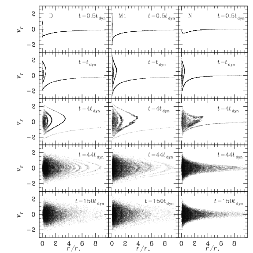
Figure 4.— Phase-space (radial-velocity vs. radius) diagrams for simulations D, M1, and N at various times. $v_{r}$ is in units of $v_{\rm*d}$ (simulation D), and $v_{\rm*n}$ (simulations M1 and N; see Table 1).

Figure 5.— Initial (top) and final (bottom) differential energy distributions. The energy per unit mass $E$ is in units of $E_{\rm*d}/{M_{*}}$ (model D), and $E_{\rm*n}/{M_{*}}$ (models M1 and N). The energy zero points in models D and M1 are such that the most bound particles of the M1 and N end-products have the same energy, and the highest energy particles of models D and M1 at $t=0$ have the same energy.

To explore the phase-space evolution of the systems during the collapse and the following relaxation we consider time snapshots of the particles radial velocity ($v_{r}$) vs. radius as in Londrillo et al. (1991). In Fig. 4 we plot five of these diagrams for simulations D, M1 and N: each plot shows the phase-space coordinates of 32000 particles randomly extracted from the corresponding simulation, and, as in Fig. 1, times are normalized to the dynamical time $t_{\rm dyn}$ (see Section 3.1). At time $t=0.5t_{\rm dyn}$ all particles are still collapsing in simulation N, while in MOND simulations a minority of particles have already crossed the center of mass, as revealed by the vertical distribution of points at $r\sim 0$ in panels D and M1. At $t=t_{\rm dyn}$ (time of the peak of $2K/|W|$ in the three models), sharp shells in phase space are present, indicating that particles are moving in and out collectively and phase mixing has not taken place yet. At $t=4t_{\rm dyn}$ is already apparent that phase mixing is operating more efficiently in simulation N than in simulation M1, while there is very little phase mixing in the dMOND collapse. At significantly late times ($t=44t_{\rm dyn}$), when the three systems are almost virialized ($2K/|W|\sim 1$; see Fig. 1), phase mixing is complete in simulation N, but phase-space shells still survive in models M1 and D. Finally, the bottom panels show the phase-space diagrams at equilibrium ($t=150t_{\rm dyn}$), when phase mixing is completed also in the MOND and dMOND galaxies: note that the populated region in the ($r$,$v_{r}$) space is significantly different in MOND and in Newtonian gravity, consistently with the sharper decline of radial velocity dispersion in the Newtonian system.

Thus, our results indicate that phase mixing is more effective in Newtonian gravity than in MOND. It is then interesting to estimate in physical units the phase-mixing timescales of MOND systems. From Table 1 it follows that $t_{\rm*n}\simeq 4.7\,(r_{*}/\rm\,kpc)^{3/2}({M_{*}}/10^{10}M_{\odot})^{-1/2}\rm\,Myr=29.8\kappa^{-3/4}({M_{*}}/10^{10}M_{\odot})^{1/4}\rm\,Myr$ for $a_{0}=1.2\times 10^{-10}{\rm m}\,{\rm s}^{-2}$. For example, in the case of model M1, adopting ${M_{*}}=10^{12}M_{\odot}$ (and $r_{*}=\sqrt{G{M_{*}}/a_{0}}\simeq 34\rm\,kpc$), shells in phase space are still apparent after $\sim 8.3\rm\,Gyr$ ($\simeq 44t_{\rm dyn}$). Simulation M1 might also be interpreted as representing a dwarf elliptical galaxy of, say, ${M_{*}}=10^{9}M_{\odot}$ (and $r_{*}=\sqrt{G{M_{*}}/a_{0}}\simeq 1.1\rm\,kpc$). In this case $44t_{\rm dyn}\sim 1.5\rm\,Gyr$. We conclude that in some MOND systems substructures in phase space can survive for significantly long times.

In addition to the ($r$,$v_{r}$) diagram, another useful diagnostic to investigate phase-space properties of gravitational systems is the energy distribution $N(E)$ (i.e. the number of particles with energy per unit mass between $E$ and $E+dE$; e.g., Binney & Tremaine 1987; Trenti & Bertin 2005). Independently of the force law, the energy per unit mass of a particle orbiting at ${\bf x}$ with speed $v$ in a gravitational potential $\phi({\bf x})$ is $E=v^{2}/2+\phi({\bf x})$, and $E$ is constant if $\phi$ is time-independent. In Newtonian gravity $\phi$ is usually set to zero at infinity for finite-mass systems, so $E<0$ for bound particles; in MOND all particles are bound, independently of their velocity, because $\phi$ is confining, and all energies are admissible. This difference is reflected in Fig. 5, which plots the initial (top) and final (bottom) differential energy distributions for simulations D, M1, and N. Given that the particles are at rest at $t=0$, the initial $N(E)$ depends only on the structure of the gravitational potential, and is significantly different in the Newtonian and MOND cases. We also note that $N(E)$ is basically the same in models D and M1 at $t=0$, because model M1 is initially in dMOND regime. In accordance with previous studies, in the Newtonian case the final differential $N(E)$ is well represented by an exponential function over most of the populated energy range (Binney 1982; van Albada 1982; Ciotti 1991; Londrillo et al. 1991; NLC06). In contrast, in model D the final $N(E)$ decreases for increasing energy, qualitatively preserving its initial shape. In the case of simulation M1 it is apparent a dichotomy between a Newtonian part at lower energies (more bound particles), where $N(E)$ is exponential, and a dMOND part at higher energies, where the final $N(E)$ resembles the initial one. We interpret this result as another manifestation of a less effective phase-space reorganization in MOND than in Newtonian collapses.

4.3. Comparison with the observed scaling relations of elliptical galaxies

Figure 6.— The location of the end-products M1 (circles), M2 (squares), M4 (triangles) and ${\rm M^{\prime}}$ (stars) in the planes ${M_{*}}-R_{\rm e}$ (a), ${M_{*}}-\sigma_{0}$ (c), ${M_{*}}-m$ (d), and in the plane in which the FP is seen edge-on (b). Vertical bars account for the projection effects, while the solid symbols refer to average values between the two extremes. The thick solid lines represent the observed Kormendy (a), FJ (c), and FP (b) relations, and the thin solid lines give estimates of the corresponding scatter (Bernardi et al. 2003ab). The normalization is such that $R_{\rm e}\simeq 4\rm\,kpc$ for stellar mass ${M_{*}}=10^{11}M_{\odot}$ (Shen et al. 2003). See text for the meaning of the dotted lines.

It is not surprising that galaxy scaling relations represent an even stronger test for MOND than for Newtonian gravity, due to the absence of dark matter and the existence of the critical acceleration $a_{0}$ with a universal value in the former theory (e.g., see Milgrom 1984; Sanders 2000). For example, when interpreting the FP tilt in Newtonian gravity one can invoke a systematic and fine-tuned increase of the galaxy dark-to-luminous mass ratio with luminosity (e.g., Bender, Burstein & Faber 1992; Renzini & Ciotti 1993; Ciotti, Lanzoni & Renzini 1996), while in MOND the tilt should be related to the characteristic acceleration $a_{0}$. Note, however, that in MOND as well as in Newtonian gravity other important physical properties may help to explain the FP tilt, such as a systematic increase of radial orbital anisotropy with mass or a systematic structural weak homology (Bertin et al. 2002). Due to the relevance of the subject, we attempt here to derive some preliminary hints. In particular, for the first time, we can compare with the scaling relations of elliptical galaxies MOND models produced by a formation mechanism, yet as simple as the dissipationless collapse.

In this Section we consider the end-products of simulations M1, M2, and M4. As already discussed in Section 3, each of the three systems corresponds to a family with constant ${M_{*}}/r_{*}^{2}$. This degeneracy is represented by the straight dotted lines in Fig. 6a: all galaxies on the same dotted line have the same $\kappa$ value. This behavior is very different from the Newtonian case, in which the result of a N-body simulation can be placed anywhere in the space $R_{\rm e}-{M_{*}}$, by arbitrarily choosing ${M_{*}}$ and $r_{*}$. For comparison with observations, the specific scaling laws represented in Fig. 6 (thick solid lines) are the near-infrared $z^{*}$-band Kormendy relation $R_{\rm e}\propto{M_{*}}^{0.63}$ and FJ relation ${M_{*}}\propto\sigma_{0}^{3.92}$ (Bernardi et al. 2003a), and the edge-on FP relation in the same band $\log R_{\rm e}=A\log\sigma_{0}+B\log({M_{*}}/R_{\rm e}^{2})+const$ (with $A=1.49$, $B=-0.75$; Bernardi et al. 2003b), under the assumption of luminosity-independent mass-to-light ratio.

The physical properties of each model are determined as follows. First, for each model (identified by a value of $\kappa=G{M_{*}}/r_{*}^{2}a_{0}$) we measure the ratio $R_{\rm e}/r_{*}$ (see Section 3.1), and so we obtain $R_{\rm e}=R_{\rm e}(\kappa,{M_{*}})$. This function, for fixed $\kappa$ and variable ${M_{*}}$, is a dotted line in Fig. 6a. As apparent, only one pair $(R_{\rm e},{M_{*}})$ satisfies the Kormendy relation for each $\kappa$: in particular, we obtain that models M1, M2, and M4 have stellar masses $1.6\times 10^{12}$, $1.4\times 10^{11}$, and $10^{10}M_{\odot}$, respectively (so lower $\kappa$ models correspond to higher mass systems). We are now in the position to obtain $r_{*}=\sqrt{G{M_{*}}/a_{0}\kappa}$ and $v_{\rm*n}=(\kappa a_{0}G{M_{*}})^{1/4}$, so we know the physical value of the projected central velocity dispersion, and we can place our models also in the FJ and FP planes. It is apparent that these two relations are not reproduced, in particular by massive galaxies. We note that this discrepancy cannot be fixed even when considering the mass interval allowed by the scatter in the Kormendy relation (thin solid lines in panel a), as revealed by the dotted lines in Fig. 6bc, which are just the projections of the dotted lines in Fig. 6a onto the planes of the edge-on FP and the FJ. Finally, Fig. 6d plots the best-fit Sersic index $m$ of the models as a function of ${M_{*}}$. Observations show that elliptical galaxies are characterized by $m$ values increasing with size: $m{\,\mathrel{\mathchoice{\lower 2.9pt\vbox{\halign{$\m@th\displaystyle\hfil#\hfil$\cr>\crcr\sim\crcr}}}{\lower 2.9pt\vbox{\halign{$\m@th\textstyle\hfil#\hfil$\cr>\crcr\sim\crcr}}}{\lower 2.9pt\vbox{\halign{$\m@th\scriptstyle\hfil#\hfil$\cr>\crcr\sim\crcr}}}{\lower 2.9pt\vbox{\halign{$\m@th\scriptscriptstyle\hfil#\hfil$\cr>\crcr\sim\crcr}}}\,}}4$ for galaxies with $R_{\rm e}{\,\mathrel{\mathchoice{\lower 2.9pt\vbox{\halign{$\m@th\displaystyle\hfil#\hfil$\cr>\crcr\sim\crcr}}}{\lower 2.9pt\vbox{\halign{$\m@th\textstyle\hfil#\hfil$\cr>\crcr\sim\crcr}}}{\lower 2.9pt\vbox{\halign{$\m@th\scriptstyle\hfil#\hfil$\cr>\crcr\sim\crcr}}}{\lower 2.9pt\vbox{\halign{$\m@th\scriptscriptstyle\hfil#\hfil$\cr>\crcr\sim\crcr}}}\,}}3\rm\,kpc$ and $m{\,\mathrel{\mathchoice{\lower 2.9pt\vbox{\halign{$\m@th\displaystyle\hfil#\hfil$\cr<\crcr\sim\crcr}}}{\lower 2.9pt\vbox{\halign{$\m@th\textstyle\hfil#\hfil$\cr<\crcr\sim\crcr}}}{\lower 2.9pt\vbox{\halign{$\m@th\scriptstyle\hfil#\hfil$\cr<\crcr\sim\crcr}}}{\lower 2.9pt\vbox{\halign{$\m@th\scriptscriptstyle\hfil#\hfil$\cr<\crcr\sim\crcr}}}\,}}4$ for those with $R_{\rm e}{\,\mathrel{\mathchoice{\lower 2.9pt\vbox{\halign{$\m@th\displaystyle\hfil#\hfil$\cr<\crcr\sim\crcr}}}{\lower 2.9pt\vbox{\halign{$\m@th\textstyle\hfil#\hfil$\cr<\crcr\sim\crcr}}}{\lower 2.9pt\vbox{\halign{$\m@th\scriptstyle\hfil#\hfil$\cr<\crcr\sim\crcr}}}{\lower 2.9pt\vbox{\halign{$\m@th\scriptscriptstyle\hfil#\hfil$\cr<\crcr\sim\crcr}}}\,}}3\rm\,kpc$ (e.g. Caon, Capaccioli & d’Onofrio 1993). Our models behave in the opposite way, as $m$ decreases for increasing size (mass) of the system. So, while model M4 ($R_{\rm e}\sim 1\rm\,kpc$, $m\sim 3.4$) is consistent with observations, models M1 and M2 have significantly lower $m$ than real ellipticals of comparable size. However, this finding is not a peculiarity of MOND gravity: also in Newtonian gravity dissipationless collapse end-products with $m>4$ are obtained only for specific initial conditions (NLC06), while equal mass Newtonian mergings are able to produce high-$m$ systems (Nipoti et al. 2003).

So far we have compared the results of our simulations with the scaling relations of high-surface brightness galaxies. However, it is well known that low surface-brightness hot stellar systems, such as dwarf ellipticals and dwarf spheroidals, have larger effective radii than predicted by the Kormendy relation (e.g., Bender et al. 1992; Capaccioli, Caon & d’Onofrio 1992; Graham & Guzmán 2003). In particular, dwarf ellipticals are characterized by effective surface densities comparable to those of the most luminous ellipticals, while their surface brightness profiles are characterized by Sersic indices smaller than $4$ (e.g. Caon et al. 1993; Trujillo, Graham, & Caon 2001). Dwarf spheroidals are the lowest surface-density stellar systems known, and typically have exponential ($m\sim 1$) luminosity profiles (e.g. Mateo 1998). So, simulations M1 and D can be interpreted as modeling a dwarf elliptical and a dwarf spheroidal, respectively, and their end-products qualitatively reproduce the surface brightness profiles of the observed systems. As pointed out in Section 4.1.2, the velocity-dispersion profile of model D is rather flat, with a hole in the central regions: interestingly observations of dwarf spheroidals indicate that their velocity-dispersion profiles are also flat (e.g. Walker et al. 2006 and references therein).

5. Discussion and conclusions

In this paper we studied the dissipationless collapse in MOND by using a new three-dimensional particle-mesh N-body code, which solves the MOND field equation (2) exactly. For obvious computational reasons, we did not attempt a complete exploration of the parameter space, and we just presented results of a small set of numerical simulations, ranging from Newtonian to dMOND systems. The main results of the present study can be summarized as follows:

• The intrinsic structural and kinematical properties of the MOND collapse end-products depend weakly on their characteristic surface density: lower surface-density systems have shallower inner density profile, flatter velocity-dispersion profile, and more radially anisotropic orbital distribution than higher surface-density systems.

• The projected density profiles of the MOND collapse end-products are characterized by Sersic index $m$ lower than $4$, and decreasing for decreasing mean surface density. In particular, the end-product of the dMOND collapse, modeling a very low surface density system, is characterized by a Sersic index $m\sim 2$ and by a central hole in the projected velocity-dispersion profile.

• We found impossible to satisfy simultaneously the observed Kormendy, Faber-Jackson and Fundamental Plane relations of elliptical galaxies with the MOND collapse end-products, under the assumption of a luminosity independent mass-to-light ratio. In other words, this point and the two points above show that, in the framework of dissipationless collapse, the presence of a characteristic acceleration is not sufficient to reproduce important observed properties of spheroids of different mass and surface density, such as their scaling relations and weak structural homology.

• From a dynamical point of view we found that phase mixing is less effective (and stellar systems take longer to relax) in MOND than in Newtonian gravity.

A natural question to ask is how the end-products of our simulations would be interpreted in the context of Newtonian gravity. Clearly, models D and N would represent dark-matter dominated and baryon dominated stellar systems, respectively. More interestingly, models M1, M2, and M4, once at equilibrium, would be characterized by a dividing radius, separating a baryon-dominated inner region (with accelerations higher than $a_{0}$) from a dark-matter dominated outer region (with accelerations lower than $a_{0}$). This radius is $\sim 1.1r_{\rm h}$ for M1, $\sim 1.8r_{\rm h}$ for M2, and $\sim 2.7r_{\rm h}$ for M4. So, all these models would show little or no dark matter in their central regions. Remarkably, observational data indicate that there is at most as much dark matter as baryonic matter within the effective radius of ellipticals (e.g. Bertin et al. 1994; Cappellari et al. 2006 and references therein).

The conclusions above have been drawn by considering only simulations starting from an inhomogeneous Plummer density distribution. To explore the dependence of these results on this specific choice, we ran also three simulations starting from a cold ($2K/|W|=0$), inhomogeneous and truncated density distribution $\rho(r)=C{M_{*}}/(r_{*}^{3}+r^{3})$, where $C^{-1}\equiv 4\pi\ln(1+r_{\rm t}^{3}/r_{*}^{3})/3$, ${M_{*}}$ is the total mass, and $r_{\rm t}=20r_{*}$ is the truncation radius. Inhomogeneities are introduced as described in Section 3.1. Note that in the external parts the new initial conditions are significantly flatter than a Plummer sphere. The three simulations are labeled ${\rm D^{\prime}}$ (dMOND), ${\rm M^{\prime}}$ (MOND with acceleration ratio $\kappa=20$) and ${\rm N^{\prime}}$ (Newtonian). As in the case of Plummer initial conditions, also in these cases the final intrinsic and projected density distributions are well represented by $\gamma$-models and Sersic models, respectively. In analogy with model N, the Newtonian collapse ${\rm N^{\prime}}$ produced the system with the steepest central density distribution (see Table 2). In addition, model ${\rm M^{\prime}}$, when compared with the scaling laws of ellipticals (stars in Fig. 6), follows the same trend as models M1, M2 and M4. The analysis of the time-evolution in phase-space of models ${\rm D^{\prime}}$, ${\rm M^{\prime}}$ and ${\rm N^{\prime}}$ confirmed that mixing and relaxation processes are less effective in MOND than in Newtonian gravity.

How do the presented results depend on the specific choice (equation 5) of the MOND interpolating function $\mu$? Recently, a few other interpolating functions have been proposed to better fit galactic rotation curves (Famaey & Binney 2005), and in the context of TeVeS (Bekenstein 2004; Zaho & Famaey 2006). It is reasonable to expect that the exact form of $\mu$ is not critical in a violent dynamical process such as dissipationless collapse. We verified that this is actually the case, by running an additional MOND simulation with the same initial conditions and parameter $\kappa$ as simulation M1, but adopting $\mu(y)=y/(1+y)$, as proposed by Famaey & Binney (2005). In fact, neither in the time-evolution nor in the structural and kinematical properties of the end-products we found significant differences between the two simulations. This result suggests that, in the context of structure formation in MOND, the crucial feature is the presence of a characteristic acceleration separating the two gravity regimes, while the details of the transition region are unimportant.

Though the dissipationless collapse is a very simplistic model for galaxy formation, it is expected to describe reasonably well the last phase of “monolithic-like” galaxy formation, in which star formation is almost completed during the initial phases of the collapse. The importance of gas dissipation in the formation of elliptical galaxies is very well known, going back to the seminal works of Rees & Ostriker (1977) and White & Rees (1978; see also Ciotti, Lanzoni & Volonteri 2006, and references therein, for a discussion of the expected impact of gas dissipation on the scaling laws followed by elliptical galaxies). This aspect has been completely neglected in our exploration, and we are working on an hybrid (stars plus gas) version of the MOND code to explore quantitatively this issue. We also stress that the dissipationless collapse process catches the essence of violent relaxation, which is certainly relevant to the formation of spheroids even in more complicated scenarios, such as merging. For example, it is well known that in Newtonian dynamics systems with de Vaucouleurs profiles are produced by dissipationless merging of spheroids (e.g. White 1978) or disk galaxies (e.g. Barnes 1992) as well as by dissipationless collapses (van Albada 1982). Merging simulations in MOND have not been performed so far, and a relevant and still open question is how efficient merging is in MOND, in which the important effect of dark matter halos is missing, and galaxies are expected to collide at higher speed than in Newtonian gravity (Binney 2004; Sellwood 2004). Our results, indicating that relaxation takes longer in MOND than in Newtonian gravity, go in the direction of making merging time scales even longer in MOND; on the other hand, analytical estimates seem to indicate shorter dynamical friction time-scales in MOND than in Newtonian gravity (Ciotti & Binney 2004). So, the next application of our code will be the study of galaxy merging in MOND.

Appendix A The volume-limited energy-balance equation in MOND

In this Appendix we derive a useful volume-limited integral relation representing energy conservation in MOND, well suited to test numerical simulations. The total (ordered and random) kinetic energy per unit volume of a continuous distribution with density $\rho$ and velocity field ${\bf u}$ is

$$k={\rho\over 2}(||{\bf u}||^{2}+{\rm Tr}\,{\sigma^{2}_{ij}}),$$ (A1)

where $\sigma^{2}_{ij}$ is the velocity-dispersion tensor. In the present case the energy balance equation is (e.g. Ciotti 2000)

$${d\over dt}\int_{V(t)}kd^{3}{\bf x}=-\int_{V(t)}\rho{\bf u}\cdot\nabla\phi d^{3}{\bf x},$$ (A2)

where the integral in the r.h.s. is the work per unit time done by mechanical forces. By application of the Reynolds transport theorem and using the mass continuity equation we obtain

$${\partial\over\partial t}(k+\rho\phi)+\nabla\cdot[(k+\rho\phi){\bf u}]=\rho{\partial\phi\over\partial t}.$$ (A3)

When $\phi$ is the MOND gravitational potential, $\rho$ can be eliminated using equation (2), so

$$4\pi G\rho{\partial\phi\over\partial t}=\nabla\cdot(\mu\nabla\phi){\partial\phi\over\partial t}=\nabla\cdot\left(\mu\nabla\phi{\partial\phi\over\partial t}\right)-{a_{0}^{2}\over 2}{\partial\over\partial t}\left[\mathcal{F}\left({||\nabla\phi||\over a_{0}}\right)\right],$$ (A4)

where $\mathcal{F}$ is defined in equation (9). Thus, equation (A3) can be written as

$${\partial\over\partial t}\left[k+\rho\phi+{a_{0}^{2}\over 8\pi G}\mathcal{F}\left({||\nabla\phi||\over a_{0}}\right)\right]+\nabla\cdot\left[(k+\rho\phi){\bf u}-{\mu\nabla\phi\over 4\pi G}{\partial\phi\over\partial t}\right]=0.$$ (A5)

By integration over a fixed control volume $V_{0}$ enclosing all the system mass one obtains equation (2).

Appendix B The virial trace $W$ in deep-MOND systems of finite mass

Here we prove that $W=-(2/3)\sqrt{Ga_{0}M_{*}^{3}}$ for any dMOND system of finite mass ${M_{*}}$. Eliminating $\rho$ from equation (11) by using equation (6), and considering the trace of the resulting expression one finds

$$W=-{1\over 4\pi Ga_{0}}\int{\cal D}[\phi]\nabla\cdot\left({\|\nabla\phi\|}\nabla\phi\right)d^{3}{\bf x},$$ (B1)

where we define the operator ${\cal D}\equiv<{\bf x},\nabla>$. The remarkable fact behind the proof is that the integrand above can be written as the divergence of a vector field, so only contributions from $r\to\infty$ are important. We will then use the spherically symmetric asymptotic behavior of dMOND solutions for $r\to\infty$ (BM)

$${\bf g}=-\nabla\phi\sim-{\sqrt{G{M_{*}}a_{0}}\over r}\hat{\bf e}_{r}$$ (B2)

and Gauss theorem to evaluate $W$.

Theorem. For a generic potential the following identity holds:

$${\cal D}[\phi]\nabla\cdot({\|\nabla\phi\|}\nabla\phi)=\nabla\cdot\left({\cal D}[\phi]{\|\nabla\phi\|}\nabla\phi-{{\bf x}{\|\nabla\phi\|}^{3}\over 3}\right).$$ (B3)

Proof. From standard vector analysis (e.g. Jackson 1999) it follows that

$${\cal D}[\phi]\nabla\cdot\left({\|\nabla\phi\|}\nabla\phi\right)=\nabla\cdot\left({\cal D}[\phi]{\|\nabla\phi\|}\nabla\phi\right)-{\|\nabla\phi\|}<\nabla\phi,\nabla{\cal D}[\phi]>,$$ (B4)

and

$${\|\nabla\phi\|}<\nabla\phi,\nabla{\cal D}[\phi]>={\nabla\cdot\left({\bf x}{\|\nabla\phi\|}^{3}\right)\over 3}.$$ (B5)

Identity (B5) follows from the expansion $\nabla{\cal D}[\phi]=\nabla\phi+{\cal D}[\nabla\phi]$ as

$${\|\nabla\phi\|}^{3}+{\|\nabla\phi\|}<\nabla\phi,{\cal D}[\nabla\phi]>={\|\nabla\phi\|}^{3}+{{\cal D}\left[{\|\nabla\phi\|}^{3}\right]\over 3}={\nabla\cdot\left({\bf x}{\|\nabla\phi\|}^{3}\right)\over 3}.$$ (B6)

Combining equations (B4) and (B5) completes the proof of equation (B3).

We now transform the volume integral (B1) in a surface integral over a sphere of radius $r$, and we consider the limit for $r\to\infty$ together with the asymptotic relation (B2), obtaining

$$W=-{1\over 4\pi Ga_{0}}\lim_{r\to\infty}\int_{4\pi}{2\over 3}r^{3}g^{2}d\Omega=-{2\over 3}\sqrt{Ga_{0}M_{*}^{3}}.$$ (B7)

Appendix C Scaling of the equations

Given a generic density distribution $\rho$, and the mass and length units ${M_{*}}$ and $r_{*}$, we define the dimensionless quantities $\tilde{{\bf x}}\equiv{\bf x}/r_{*}$, and $\tilde{\rho}\equiv\rho r_{*}^{3}/{M_{*}}$. From equation (3) the equation of motion for a test particle can be written in dimensionless form as

$${d^{2}\tilde{{\bf x}}\over d\tilde{t}^{2}}=-{\phi_{*}t_{*}^{2}\over r_{*}^{2}}\tilde{\nabla}\tilde{\phi},$$ (C1)

where $\phi_{*}$ and $t_{*}$ are for the moment two unspecified scaling constants, $\tilde{\phi}=\phi/\phi_{*}$ and $\tilde{t}=t/t_{*}$, and the dimensionless gradient operator is $\tilde{\nabla}=r_{*}\nabla$. In all of our simulations we define $t_{*}\equiv r_{*}/\sqrt{\phi_{*}}$, so that the scaling factor in equation (C1) is unity, while $\phi_{*}$ is specified case-by-case from the field equation as follows.

In Newtonian gravity the Poisson equation (1) can be written as

$$\tilde{\nabla}^{2}\tilde{\phi}=4\pi{G{M_{*}}\over r_{*}\phi_{*}}\tilde{\rho}:$$ (C2)

we fix $\phi_{*}=G{M_{*}}/r_{*}$, so $t_{*}=\sqrt{r_{*}^{3}/G{M_{*}}}\equiv t_{\rm*n}$. The dMOND field equation (6) in dimensionless form writes

$$\tilde{\nabla}\cdot(||\tilde{\nabla}\tilde{\phi}||\tilde{\nabla}\tilde{\phi})=4\pi{G{M_{*}}a_{0}\over\phi_{*}^{2}}\tilde{\rho},$$ (C3)

so the natural choice is $\phi_{*}=\sqrt{G{M_{*}}a_{0}}$, and $t_{*}=r_{*}(G{M_{*}}a_{0})^{-1/4}\equiv t_{\rm*d}$. Finally, the MOND field equation (2) in dimensionless form is

$$\tilde{\nabla}\cdot\left[\mu(\kappa||\tilde{\nabla}\tilde{\phi}||)\tilde{\nabla}\tilde{\phi}\right]=4\pi{G{M_{*}}\over r_{*}\phi_{*}}\tilde{\rho},$$ (C4)

where $\kappa\equiv\phi_{*}/r_{*}a_{0}$. In this case, as in the Newtonian case, $\phi_{*}=G{M_{*}}/r_{*}$, so $t_{*}=t_{\rm*n}$ and $\kappa=G{M_{*}}/r_{*}^{2}a_{0}$.

References

- (1) Aguilar, L.A., & Merritt, D. 1990, ApJ, 354, 33
- (2) Barnes, J. 1992, ApJ, 393, 484
- (3) Barnes, J.E., & Hut, P. 1986, Nature, 324, 446
- (4) Bekenstein, J. 2004, Phys. Rev. D, 70, 083509
- (5) Bekenstein, J., & Milgrom, M. 1984, ApJ, 286, 7 (BM)
- (6) Bender, R., Burstein, D., & Faber, S.M. 1992, ApJ, 399, 462
- (7) Bernardi M., et al. 2003a, AJ, 125, 1849
- (8) Bernardi M., et al. 2003b, AJ, 125, 1866
- (9) Bertin, G., Ciotti, L., & Del Principe, M. 2002, A&A, 386, 1491
- (10) Bertin, G., et al. 1994, A&A, 292, 381
- (11) Binney, J. 1982, MNRAS, 200, 951
- (12) Binney, J. 2004, in Ryder, S.D., Pisano, D.J., Walker, M.A., Freeman, K.C., eds, IAU Symp. 220, Dark Matter in Galaxies. Astron. Soc. Pac., San Francisco, p. 3
- (13) Binney, J., & Tremaine, S. 1987, Galactic Dynamics (Princeton: Princeton University Press)
- (14) Brada, R., & Milgrom, M. 1995, MNRAS, 276, 453
- (15) Brada, R., & Milgrom, M. 1999, ApJ, 519, 590
- (16) Brada, R., & Milgrom, M. 2000, ApJ, 541, 556
- (17) Caon, N., Capaccioli, M., & D’Onofrio, M. 1993, MNRAS, 265, 1013
- (18) Capaccioli, M., Caon N., & D’Onofrio, M. 1992, MNRAS, 259, 323
- (19) Cappellari M., et al., 2006, MNRAS, 366, 1126
- (20) Christodoulou, D.M. 1991, ApJ, 372, 471
- (21) Ciotti, L. 1991, A&A, 249, 99
- (22) Ciotti, L. 2000, Lecture Notes on Stellar Dynamics (Pisa: Scuola Normale Superiore editor)
- (23) Ciotti, L., & Bertin, G. 1999, A&A, 352, 447
- (24) Ciotti, L., & Binney, J. 2004, MNRAS, 351, 285
- (25) Ciotti, L., Lanzoni, B., & Renzini, A. 1996, MNRAS, 282, 1
- (26) Ciotti, L., Lanzoni, B., & Volonteri, M. 2006, ApJ, in press (astro-ph/0611328)
- (27) Ciotti, L., Londrillo, P., & Nipoti, C. 2006, ApJ, 640, 741 (CLN)
- (28) Ciotti, L., Nipoti, C., & Londrillo, P. 2007, in proceedings of the International Workshop “Collective phenomena in macroscopic systems” (Como, Italy, December 4-6, 2006)
- (29) de Vaucouleurs, G. 1948, Ann. d’Astroph., 11, 247
- (30) Dehnen, W. 1993, MNRAS, 265, 250
- (31) Dehnen, W. 2002, Journal of Computational Physics, 179, 27
- (32) Djorgovski, S., & Davis, M. 1987, ApJ, 313, 59
- (33) Dressler, A., Lynden-Bell, D., Burstein, D., Davies, R.L., Faber, S.M., Terlevich, R., & Wegner, G. 1987, ApJ, 313, 42
- (34) Faber, S.M., & Jackson, R.E. 1976, ApJ, 204, 668
- (35) Famaey, B., & Binney, J. 2005, MNRAS, 363, 603
- (36) Felten, J.E. 1984, ApJ, 286, 3
- (37) Gerhard, O.E., & Spergel, D.N. 1992, ApJ, 397, 38
- (38) Graham, A.W., & Guzmán, R. 2003, AJ, 125, 2936
- (39) Gunn, J.E., & Gott, J.R. 1972, ApJ, 176, 1
- (40) Hockney, R., & Eastwood, J. 1988, Computer Simulation Using Particles (Bristol: Hilger)
- (41) Jackson, J.D. 1999, Classical Electrodynamics (New York: New John Wiley & Sons, Inc.)
- (42) Knebe, A., & Gibson, B.K. 2004, MNRAS, 347, 1055
- (43) Kormendy J., 1977, ApJ, 295, 73
- (44) Londrillo, P., Messina, A., & Stiavelli, M. 1991, MNRAS, 250, 54
- (45) Londrillo, P., Nipoti, C., & Ciotti, L. 2003, In “Computational astrophysics in Italy: methods and tools”, Roberto Capuzzo-Dolcetta ed., Mem. S.A.It. Supplement, vol. 1, p. 18
- (46) Lynden-Bell, D. 1967, MNRAS, 136, 101
- (47) Mateo, M.L. 1998, ARA&A, 36, 435
- (48) Milgrom, M. 1983, ApJ, 270, 365
- (49) Milgrom, M. 1984, ApJ, 287, 571
- (50) Milgrom, M. 2002, New. Astron. Rev., 46, 741
- (51) Nipoti, C., Londrillo, P., & Ciotti, L. 2002, MNRAS, 332, 901
- (52) Nipoti, C., Londrillo, P., & Ciotti, L. 2003, MNRAS, 342, 501
- (53) Nipoti, C., Londrillo, P., & Ciotti, L. 2006, MNRAS, 370, 681 (NLC06)
- (54) Nusser, A. 2002, MNRAS, 331, 909
- (55) Nusser, A., & Pointecouteau, E. 2006, MNRAS, 366, 96
- (56) Plummer, H.C. 1911, MNRAS, 71, 460
- (57) Power, C., Navarro, J.F., Jenkins, A., Frenk, C.S., White, S.D.M., Springel, V., Stadel, J., & Quinn, T. 2003, MNRAS, 338, 14
- (58) Rees, M.J., & Ostriker, J.P. 1977, MNRAS, 179, 541
- (59) Renzini A., Ciotti L., 1993 ApJ, 416, L49
- (60) Sanders, R.H. 2000, MNRAS, 313, 767
- (61) Sanders, R.H., & McGaugh, S.S. 2002, ARA&A, 40, 263
- (62) Sellwood, J. 2004, in Ryder, S.D., Pisano, D.J., Walker, M.A., Freeman, K.C., eds, IAU Symp. 220, Dark Matter in Galaxies. Astron. Soc. Pac., San Francisco, p. 27
- (63) Sersic, J.L. 1968, Atlas de galaxias australes. Observatorio Astronomico, Cordoba
- (64) Shen, S., Mo, H.J., White, S.D.M., Blanton, M.R., Kauffmann, G., Voges, W., Brinkmann, J., & Csabai, I. 2003, MNRAS, 343, 978
- (65) Stachniewicz, S., & Kutschera, M. 2005, MNRAS, 362, 89
- (66) Tiret, O., & Combes, F. 2007, preprint (astro-ph/0701011)
- (67) Tremaine, S., Richstone, D.O., Yong-Ik, B., Dressler, A., Faber, S.M., Grillmair, C., Kormendy, J., & Laurer, T.R. 1994, AJ, 107, 634
- (68) Trenti, M., & Bertin, G. 2005, A&A, 429, 161
- (69) Trenti, M., Bertin, G., & van Albada, T.S. 2005, A&A, 433, 57
- (70) Trujillo, I., Graham, A.W., & Caon, N. 2001, MNRAS, 326, 869
- (71) Udry, S. 1993, A&A, 268, 35
- (72) van Albada, T.S. 1982, MNRAS, 201, 939
- (73) Walker, M.G., Mateo, M., Olszewski, E.W., Pal, J.K., Sen, B., & Woodroofe, M. 2006, ApJ, 642, L41
- (74) White, S.D.M 1978 MNRAS, 184, 185
- (75) White, S.D.M, & Rees, M.J., 1978, MNRAS, 183, 341
- (76) Zaho, H., & Famaey, B. 2006, ApJ, 638, L9