Toward a New Geometric Distance to the Active Galaxy NGC 4258:
I. VLBI Monitoring of Water Maser Emission

Abstract

We report a three year, 18 epoch, VLBI monitoring study of H₂O masers in the sub-parsec, warped, accretion disk within the NGC 4258 AGN. Our immediate goals are to trace the geometry of the underlying disk, track rotation via measurement of proper motion, and ascertain the radii of masers for which centripetal acceleration may be measured separately. The monitoring includes $\sim 4\times$ as many epochs, $\sim 3\times$ denser sampling, and tighter control over sources of systematic error than earlier VLBI investigations. Coverage of a $\sim 2400$ km s^-1 bandwidth has also enabled mapping of molecular material $\sim 30\%$ closer to the black hole than accomplished previously, which will strengthen geometric and dynamical disk models. Through repeated observation we have also measured for the first time a $5\mu$as ($1\sigma$) thickness of the maser medium. Assuming this corresponds to the thickness of the accretion disk, hydrostatic equilibrium requires a disk plane temperature of $\approx$ 600 K. Our long-term goal is a geometric distance to NGC 4258 that is accurate to $\sim 3\%$, a $\sim 2\times$ improvement over the current best estimate. A geometric estimate of distance can be compared to distances obtained from analysis of Cepheid light curves, with the intent to recalibrate the extragalactic distance scale with reduced systematic uncertainties. This is the first paper in a series. We present here VLBI observations, data reduction, and temporal and spatial characteristics of the maser emission. Later papers will report estimation of orbital acceleration and proper motion, modeling of disk 3-D geometry and dynamics, and estimation of a “ maser distance.” Estimation of a “Cepheid distance” is presented in a parallel paper series.

1 Introduction

The extragalactic distance scale (EDS) is underpinned by measurements of “standard candles” in the Large Magellanic Cloud (LMC) and other nearby galaxies (Freedman et al., 2001). The long-term importance of a high-accuracy EDS calibration lies in potential precision estimation of cosmological parameters, such as the equation of state for dark energy (e.g., Hu, 2005). One means by which the EDS calibration might be improved is by anchoring “standard candle” calibration to distances estimated by geometric techniques. Towards this end, NGC 4258—for which a geometric distance has been estimated from modelling of the 3-D geometry and dynamics of the accretion disk surrounding the central engine (Herrnstein et al., 1999)—could either replace or be used in conjunction with the LMC as anchor.

In NGC 4258, accretion disk material emits H₂O maser emission in the $6_{16}-5_{23}$ transition at 22.235 GHz, which was first reported close to the systemic velocity ($V_{sys}$) by Claussen et al. (1984). A key discovery was high-velocity Doppler components at $\sim V_{sys}\pm 1000$ km s^-1 (Nakai, Inoue, & Miyoshi, 1993) in NGC 4258, where $V_{sys}=472\pm 4$ km s^-1, adopting the Local Standard of Rest (LSR) and radio definition of Doppler shift (Cecil, Wilson, & Tully, 1992). An early Very Long Baseline Interferometry (VLBI) study (Greenhill et al., 1995a) suggested that maser emission might originate from a rotating disk, as did a parallel investigation of secular velocity drifts for the peaks of spectral features, i.e., centripetal accelerations (Haschick, Baan, & Peng 1994; Greenhill et al. 1995b; Nakai et al. 1995; see also Watson & Wallin 1994). Low-velocity Doppler components (those near $V_{sys}$) drifted by $\approx+10$ km s^-1 yr^-1 and high-velocity components drifted by $<\pm 1$ km s^-1 yr^-1, thus localizing the former to the near side of the disk and the latter near the mid-line (i.e., the diameter perpendicular to the line of sight). The sub-parsec disk model was confirmed by Very Long Baseline Array (VLBA) observations, which traced, most importantly, the disk warp and the rotation curve, the latter being Keplerian to better than 1% (Miyoshi et al. 1995; see also Herrnstein et al. 2005).

For a Keplerian system, accurate first-order estimates of geometric distance may be obtained relatively simply from the geometry of the warped disk and measurements of acceleration or proper motion for low-velocity emission. To date, NGC 4258 is the only galaxy for which this has been done. Herrnstein et al. (1999) obtained a distance to NGC 4258 of $7.2\pm 0.3~{}(random)\pm 0.4~{}(systematic)$ Mpc, where the systematic term is due mostly to a thus far weak constraint on orbital eccentricity ($<0.1$). Our major aim is to reduce both random and systematic error. Herrnstein et al. (1999) used four epochs of VLBA data spanning 3 years to estimate distance. In contrast, we have 18 epochs over a subsequent 3.4 year interval. This facilitates more detailed modeling of disk substructure, formal incorporation of orbital eccentricity and periapsis angle as parameters, more definitive tracking of disk rotation, and reduction of random and systematic error by a factor of at least two. Humphreys et al. (2005) discuss early progress.

The current distance scale, as characterized by the Hubble constant (H_∘), may be uncertain by perhaps as little as 10% (Freedman et al., 2001). The most robust estimate depends on measured mean magnitudes of $\sim 800$ Cepheid variable stars in 31 galaxies within 30 Mpc, and comparison with the period luminosity (PL) relation for Cepheids in the Large Magellanic Cloud (LMC). The LMC establishes a zero point for calibration of Cepheid light curves in other galaxies. Common secondary distance indicators that are identifiable in the Hubble Flow (e.g., Tully Fisher relation, type Ia SNe), are calibrated using distances to Cepheid host galaxies and are used in turn to estimate H_∘. High-precision estimates of H_∘ are also available from analysis of Cosmic Microwave Background (CMB) fluctuations (e.g., Spergel et al., 2006). However, degeneracies in analysis of CMB data do not allow independent determination of both H_∘ and the equation of state for dark energy, $w$. Note that Spergel et al. (2006) assumed a flat universe with $w=-1$ and obtained a value of H_∘ in good agreement with Freedman et al. (2001).

The most substantial problem with the current Cepheid-based calibration of the EDS is dependence on the LMC as zero point anchor for PL relations. Contributing factors include uncertainty in distance to the LMC, poorly understood internal galactic structure, and controversy over the impact of the difference in stellar metallicity between the LMC and HST Cepheid-sample galaxies.

The adopted uncertainty in the LMC distance by Freedman et al. (2001) is $\sim 5\%$. However, LMC distance estimates obtained from different calibrations and analyses over the last decade cover a $\pm 23\%$ range ($\pm 0.50$ mag when expressed in terms of distance moduli). This is well beyond uncertainties for individual measurements (Figure 8 of Benedict et al., 2002a) and likely indicative of unresolved systematic errors. Although uncertainties $\ll 10\%$ have been obtained from the distributions of distance estimates for different subsamples of measurements (e.g., Freedman et al., 2001; Benedict et al., 2002b), in the face of apparently unresolved systematics, the averages and moments may be statistically problematic.

The uncertain structure of the LMC (e.g., disk eccentricity, out-of-plane stellar component), complicates interpretation of distance indicators (van der Marel, 2001; Nikolaev et al., 2004, and references therein). For instance, robust estimates of distance have been obtained for eclipsing binaries, with individual uncertainties of 2 - 3% (e.g., Fitzpatrick et al., 2002, and references therein). However, for the four systems well studied thus far, the range of implied distances for the LMC center covers 14% (Fitzpatrick et al., 2003).

The impact of metallicity could be as large at $\pm 10\%$ in distance. Limited theoretical and empirical understanding has led to long term controversy over the magnitude and sign of the effect of metal content on Cepheid brightness (Sasselov et al., 1997; Kochanek, 1997; Kennicutt et al., 1998; Groenewegen et al., 2004; Sakai et al., 2004; Romaniello et al., 2006). Attempts to make definitive measurements have been complicated by the magnitude of observable metallicity gradients in well studied galaxies, the sizes of Cepheid samples, and the effects of reddening and crowding in low-metallicity fields at smaller galactocentric radii. Consensus theoretical models have not emerged because of computational difficulty, with some doubt as to whether or not metal content alone needs to be considered (Fiorentino et al., 2002).

Precision estimation of cosmological parameters is best achieved by multiple approaches. Hu (2005) argues that percent level accuracy in H_∘, combined with measurements of CMB fluctuations, would enable robust constraint on $w$ independent of those provided by measurements of, e.g., weak lensing and large scale structure. Spergel et al. (2006) also demonstrate the impact on estimates of curvature by independent constraint on H_∘. A new “maser distance” for NGC4258 is a first step, with the immediate goal of $\sim 3\%$. This paper is the first in a series. Here we present the VLBI data and briefly discuss general trends such as time evolution of position-velocity traces. Later work will present time-series maser spectroscopy and modeling of the combined datasets to obtain an improved geometric distance (cf. Herrnstein et al., 1999). Parallel analysis of recent Cepheid photometry obtained with the Hubble Space Telescope, beginning with Macri et al. (2007), will provide an improved “Cepheid distance” (cf. Newman et al., 2001). Ultimately, the two programs will culminate in comparison of maser and Cepheid distances and re-assessment of the EDS and implications for cosmology.

2 Observations and Data Reduction

2.1 The Observations

The design of the observing program was intended to enable (1) unambiguous tracking of evolution in the source spectrum and disk structure, through close spacing of epochs; (2) monitoring to detect possible transient emission outside the historically recognized velocity range of the maser, i.e., three 200 km s^-1-wide line complexes distributed over $\sim 2000$ km s^-1 (e.g., Bragg et al., 2000); (3) tight control over sources of systematic error; and (4) relatively uniform sensitivity from epoch to epoch.

We observed NGC 4258 18 times between 1997 March 6 and 2000 August 12, using the VLBA, the Very Large Array (VLA), and the Effelsberg 100-m telescope (EFLS) of the Max-Planck-Institut für Radioastronomie (Table 1). Twelve “medium-sensitivity” epochs involved the VLBA alone; the remaining six “high-sensitivity” VLBI epochs were interleaved and involved the VLBA, augmented by the phased VLA and EFLS.

In medium-sensitivity epochs, we recorded eight 16 MHz ($\approx$ 216 km s^-1) basebands with 1-bit sampling. We overlapped seven bands by 15%, resulting in observing bandpasses of $\sim 362$ to 1676 km s^-1 (covering low-velocity and red-shifted high-velocity emission) and $\sim-706$ to 608 km s^-1 (covering low-velocity and blue-shifted high-velocity emission), depending upon the epoch (Table 2). We tuned the eighth band to enable dual polarization observations of the emission peak (spanning the velocity range 362-578 km s^-1 for red-shifted epochs and 392-608 km s^-1 for blue-shifted epochs), thus increasing the signal-to-noise ratio available for tracking atmospheric and instrumental response fluctuations during calibration. Because the $\sim 2000$ km s^-1 bandwidth of the source was difficult to accommodate instantaneously with VLBI data acquisition systems, we alternated month-to-month between observing two offset $\sim 1500$ km s^-1 bands. One covered low-velocity and red-shifted high-velocity maser emission, and the other covered low-velocity and blue-shifted high-velocity emission. Combining data from adjacent months, we effectively observed $\sim 2400$ km s^-1, centered approximately on the systemic velocity.

In high-sensitivity epochs, we recorded eight 8 MHz ($\approx$ 108 km s^-1) basebands with 2-bit sampling, alternating baseband tuning over the course of each track to cover the three emission complexes. The narrower instantaneous bandwidth accommodated the limited IF bandwidth of the VLA ($2\times 50$ MHz). In the first five high-sensitivity epochs, we recorded both upper and lower sidebands to limit the number of baseband mixers required and thereby accommodate a reduced complement at Effelsberg. To avoid band gaps at mixer frequencies, we overlapped the sidebands of adjacent mixers and obtained $\approx$ 300 km s^-1 coverage of low-velocity, red-shifted, and blue-shifted emission complexes. In the last high-sensitivity epoch, we took advantage of a new complement of mixers at Effelsberg, recording only upper sidebands with 20% overlap and 365 km s^-1 coverage of each emission line complex.

2.2 Strengths of the Current Study

Time Sampling — Spacing between high-sensitivity epochs, $\sim 8$ months, was comparable to spacing between epochs in an earlier VLBI study (Herrnstein et al., 2005, their Table 1), but the 1-2 month time interval between most medium-sensitivity epochs was comparable to the typical known timescale for spectral variability (e.g., Bragg et al., 2000). A minimum 8 day separation between epochs also enabled testing for short-term source structure variability.

Bandwidth — The high-sensitivity epochs (as in all previous VLBI studies) focused on the velocity ranges in which Nakai, Inoue, & Miyoshi (1993) identified emission. In contrast, medium sensitivity observations monitored all velocities from $v_{\rm\tt LSR}\sim-706$ to 1676 km s^-1, achieving a detection threshold $\approx 2\times$ below that of earlier broadband ($-$1200 to 2650 km s^-1) single-dish studies by Nakai, Inoue, & Miyoshi (1993) and Nakai et al. (1995), scaled to the same channel spacing. Emission at “new” velocities was sought because it would presumably arise in previously unmapped portions of the accretion disk. For each epoch, we recorded eight basebands (which were correlated in two passes). Each baseband was divided into 512 spectral channels.

Quality and Consistency — The same observing setup and data reduction path were used for each medium-sensitivity epoch. A separate common setup and reduction path was used for high-sensitivity epochs. Deliberate repetition (e.g., u,v-coverage, choice and timing of calibrators, baseband tuning) limited systematic errors in differential measurements of dynamical quantities (i.e., proper motion, acceleration).

Sensitivity — Noise levels ($1\sigma$) in synthesis images were 2.3 - 4.7 mJy with a 3.0 mJy median for high-sensitivity epochs and 3.6 - 5.8 mJy with a 4.3 mJy median for medium-sensitivity epochs (Table 1). Earlier studies of low- and high-velocity emission together achieved sensitivities of 3.0 - 6.5 mJy with a 5.6 mJy median (Herrnstein et al., 2005).

2.3 Calibration and Imaging

Calibration and synthesis imaging were performed using the Astronomical Image Processing System (AIPS) software package with largely standard techniques for spectral-line VLBI. We discuss notable elements of the processing below.

2.3.1 Array and Sky Geometry

We sought to ensure consistency in the antenna coordinates used for each correlation over the 3 years of monitoring. This was achieved by implementing (post-processing) the station positions and (tectonic) velocities estimated by the United States Naval Observatory (USNO) in solution N9810 (Table 3). Because the VLA does not have dual-frequency geodetic VLBI receivers and is absent from solution N9810, we adopted a position estimated by the NRAO using single-frequency data for epoch 2000.9 and the average velocity for the nearby Pietown and Los Alamos stations (C. Walker, private communication). After correction, station positions were accurate to $\approx$ 1 mm for the VLBA and EFLS and $\approx$ 3 cm for the VLA.

To ensure consistency in the maser position and error budget from epoch to epoch, we adopted a maser position obtained from analysis of early VLBI data: $\alpha({\rm J2000})=12^{h}18^{m}57\,{\hbox to0.0pt{.\hss}}^{s}\!\,5046\pm 0\,{\hbox to0.0pt{.\hss}}^{s}\!\,0003;\ \delta({\rm J2000})=47^{\circ}18^{\prime}14\,{\hbox to0.0pt{.\hss}}{{}^{\prime\prime}}\!\,303\pm 0\,{\hbox to0.0pt{.\hss}}{{}^{\prime\prime}}\!\,003$ (Herrnstein et al., 2005). This was used in correlation of all but the first three epochs, for which we applied a frequency-dependent shift to the measured maser spot positions, after Herrnstein et al. (2005). The shift corresponded to an error of $-0\,{\hbox to0.0pt{.\hss}}^{s}\!\,0054$ and $0\,{\hbox to0.0pt{.\hss}}{{}^{\prime\prime}}\!\,033$ in right ascension and declination, respectively, in the a priori position. A priori calibrator positions were accurate to $\lesssim 1$ mas, and no corrections were made. A priori earth orientation parameters were compared to “final” values published by the USNO and found to be accuarate to $<1$ mas (pole position in X and Y) and $<0.1$ ms (UT1-UTC) for each epoch. We discuss the impact of these uncertainties and limits in $\S 2.5$ (see also Table 4).

2.3.2 Amplitude Calibration

To calibrate VLBA fringe amplitudes, we applied observatory-standard antenna gain curves and time-series system temperature measurements. An $\approx 40$% depression in the system temperatures of the red-shifted high-velocity basebands in high-sensitivity epochs rendered some of these calibrations suspect. Such large changes in system temperature is not likely and is probably due to a measurement problem. To compensate, we computed a system temperature time-series characteristic of the several low-velocity basebands and applied it to all basebands.

Accurate system temperature time-series were typically not available for the VLA and EFLS. For these two stations, we calibrated amplitudes through a comparison of fringe amplitudes on 4C39.25 among VLBA stations (after calibration) and fringe amplitudes for baselines including the VLA or EFLS. Time sampling of the resulting calibration was relatively coarse, but we anticipated later self-calibration would enable refinement.

We note that in the three cases for which we made nonstandard amplitude corrections (i.e., VLA, EFLS, and the red-shifted high-velocity VLBA basebands in high-sensitivity epochs) amplitude errors for some basebands could survive self-calibration, because gain corrections are calculated for emission in just one (low-velocity) baseband. Though a matter of concern, amplitude errors on the order of a few tens of percent on a small fraction of baselines are anticipated to have a relatively small impact on astrometry for point-like sources, i.e., maser spots.

We expect the overall flux scale for a given epoch to be accurate to $\approx 30\%$ for medium-sensitivity epochs and $\approx 50\%$ for high-sensitivity epochs. However, when comparing the overall flux scale between or among epochs, we expect an accuracy of $\approx 15\%$ for medium-sensitivity epochs and $\approx 25\%$ for high-sensitivity epochs.

2.3.3 Global Fringe fitting

The most demanding element of the global fringe fitting process was the accurate measurement of the slowly time variable electronic phase offsets among basebands, using observations of quasars made approximately every hour for that purpose. Specifically, the wide spacing in frequency among bands increased susceptibility to (nonphysical) phase wraps entering the interpolation of phase offsets between adjacent calibrator scans. Because the phase wraps were readily detected, straight-forward editing of single-band delay and rate data enabled removal and estimation of offsets with accuracies on the order of $10^{\circ}$ or $\sim 3\%$ of a fringe on the sky.

2.3.4 Self-calibration

We applied self-calibration solutions to the data in each baseband to correct for fluctuations in fringe amplitude and phase. These fluctuations arose from instabilities in the atmosphere and in the frequency standards at the stations and from antenna gain changes. For each epoch, we identified a relatively unblended Doppler component ($\mathrel{\hbox{\raise 2.15277pt\hbox{$>$}\hbox to0.0pt{\hss\lower 2.15277pt\hbox{$\sim$}}}}$ 1 Jy) to provide the reference signal. Images of the reference component achieved dynamic ranges of 40-300, defined with respect to the $5\sigma$ noise level or strongest artifact.

We observed unusually large artifacts in images of high-velocity red-shifted emission for a few high-sensitivity epochs. Dynamic ranges were reduced by a factor of $\sim 4$. We were unable to identify a cause and adopted an empirical strategy to correct the problem. For these epochs, we performed a second self-calibration on the strongest observed red-shifted Doppler component. Though typically only a few tenths of a Jy, this secondary reference was detectable because the initial self-calibration extended the phase coherence of the data. We applied the additional, slowly varying amplitude and phase corrections to the data in all red-shifted basebands. To recover relative position information (with respect to the primary reference emission), we applied the angular offset between reference features, measured prior to the second self-calibration.

Secondary self-calibration of the blue-shifted high-velocity emission was not possible because the peak flux density was too low ($<100$ mJy). We tested two secondary calibrations for the “blue data”. The first was achieved by applying the “red data” self-calibration corrections to the “blue data” and the second by applying the complex conjugate of the “red data” corrections to the “blue data”. In the first case we implicitly modeled the unexplained errors as phase-only, while in the second case as delay-only. Neither approach improved the signal-to-noise in images of blue-shifted emission, and was therefore not adopted. Some losses in imaging blue-shifted emission remain possible.

2.3.5 Imaging and Deconvolution

We imaged and CLEANed a $25.6\times 25.6$ mas field (in medium-sensitivity epochs) or a $30.72\times 30.72$ mas field (in high-sensitivity epochs) over the inner 96% of each bandpass. The known angular extent of the maser source is $\sim 1\times 16$ mas. Synthesized beam sizes and typical noise levels for individual spectral channels are given in Table 1. We used a hybrid weighting scheme midway between uniform and natural weighting (ROBUST=0 in the AIPS task IMAGR), in order to balance the desire for a small beam measured at the half-power points and low rms noise. In five of the six high-sensitivity epochs, we extended imaging outside the inner 96% of the bandpasses, because a blue-shifted Doppler component had been found in the medium-sensitivity epochs. The anticipated emission was detected in one epoch (BM081A).

2.4 Identification of Maser Spots and Continuum Emission

We fit a 2-D Gaussian brightness distribution to all peaks in channel maps and required that they satisfy the following requirements, in order to be judged bona fide maser “spots.”

• Emission centroids lie within one beamwidth over at least three adjacent channels at or above the 6$\sigma$ level.

• Fitted peak intensities exceed the intensity of imaging artifacts, i.e., intensities must exceed the local peak intensity divided by the dynamic range. We note that this dynamic range cut was only relevant to channels in high-sensitivity epochs with strong emission features and candidate secondary features.

• Half-power major and minor axes are both smaller than twice the major and minor axes of the convolving beam. In cases where breadth appeared consistent with blending of individual maser spots, we attempted to fit multi-component Gaussian models.

In each epoch, there are on the order of $10^{7}$ independent pixels among the image cubes. The probability that one or more will exceed 6$\sigma$, in the absence of a signal, is $\approx 10\%$ (e.g., Thompson, Moran, & Swenson, 2001, Fig. 9.5). By requiring three adjacent channels to satisfy this criterion, with a constraint on position, the chances of false detection are on the order of $10^{-7}$ (where we have accounted for correlation among channels consistent with the FX architecture and time-windowing of data in the VLBA correlator).

Where we had a priori information as to the location in velocity and position of a maser, we relaxed the 6$\sigma$ selection criterion. There were three instances.

• High-velocity features ($>3.5\sigma$) were accepted if emission at corresponding positions and velocities had been detected above the formal detection threshold in other epochs. The probability of false detection of a $3.5\sigma$ emission peak over one independent point (one beam) is $<10^{-3}$. Blue-shifted Doppler components falling into this category were found at $-285$ km s^-1 (BM081A), $-367$ km s^-1 (BM112G), $-373$ km s^-1 (BM081B and BM112C), and $-515$ km s^-1 (BM112C, BM112E, and BM112H). Red-shifted Doppler components falling into this category were found at 1566 km s^-1 (BM112F and BM112M).

• High-velocity blue-shifted emission ($>2\sigma$) was accepted in spectral channels adjacent to already identified blue-shifted features, if in the same epoch and at the same angular position to within a beam width. Blue-shifted emission was identified in this way at $-285$ km s^-1 (BM112C, BM112E, BM112G, BM112L, BM112N, and BM112P), $-367$ km s^-1 (BM112C), $-373$ km s^-1 (BM056C, BM112E, BM112G, BM112H, and BM112L), $-435$ km s^-1 (BM056C and BM081A), $-441$ km s^-1 (BM056C), and $-515$ km s^-1 (BM112G). The motivation for this extension of our detection limit was better establishment of line shape for weak features. It was not used to increase the number of features.

• High-velocity features ($>3.5\sigma$) outside the nominal range (i.e., Nakai, Inoue, & Miyoshi, 1993) were accepted, if single-dish study separately identified the Doppler components. In this way, we detected the 1647 km s^-1 component first reported by Modjaz et al. (2005) for epoch 2003.75. Extrapolating from the positions of other red-shifted Doppler components and adopting a Keplerian rotation curve for the “maser disk,” we confined the anticipated position of the 1647 km s^-1 emission to within 1 beam $\times$ 3 channels. Emission was detected in BM112M at 5$\sigma$ in the line-center channel and 4$\sigma$ in adjacent channels. Marginal detections were also found in two adjacent epochs, i.e., emission at 2.4 and 3.0$\sigma$ in two contiguous spectral channels for BM112K and four $2.8\sigma-3.3\sigma$ points in adjacent spectral channels for BM112O.

In addition to identifying maser emission, we searched for continuum emission at all epochs within 12.5 mas of the low-velocity reference emission. Continuum u,v-data were constructed by frequency averaging each baseband prior to imaging. In the case of BG107 and all medium-sensitivity epochs, we discarded the outer 2% of each of the red- or blue-shifted basebands and obtained an effective average of 1960 channels (30.6 and 61.3 MHz for BG107 and medium-sensitivity epochs, respectively). In the other high-sensitivity epochs, we discarded the outer 2% of each of three red- or blue-shifted basebands and averaged 1470 channels (23.0 MHz). Fewer channels were retained in these epochs, because of extensive overlap of sidebands for adjacent baseband mixers.

Finally, we performed a separate search for maser emission that might be associated with jet activity in NGC 4258, well downstream from the central engine. In the most sensitive of our high-sensitivity observations (BM112H), we boxcar averaged the u,v-data over four channels to improve sensitivity and imaged a $30.72\times 491.52$ mas ($512\times 8192$ pixels, E-W$\times$N-S) strip centered on the reference position. No emission peaks exceeded a 6$\sigma$ detection threshold (13 mJy).

2.5 The Error Budget

For each Gaussian fit, the random measurement error in position was estimated as being the larger of the fitting error or the beam full-width at half-maximum (FWHM) divided by twice the peak signal-to-noise ratio ($S/N$). We estimated the systematic position error from two components: (1) errors that scale with difference in sky frequency between a given channel and the reference (i.e., $\nu-\nu_{ref}$), and (2) errors that scale with the difference in baseband frequencies of a given channel and the reference (i.e., [$\nu-\nu_{\circ}]-[\nu_{ref}-\nu_{ref_{\circ}}]$, where $\nu_{\circ}$ and $\nu_{ref_{\circ}}$ are the band-center frequencies). The maximum difference in sky frequencies is $\approx$ 75 MHz for NGC 4258; the maximum difference in baseband frequencies is $<8$ MHz. Errors in the absolute position of the reference and calibrators, or errors in zenith propagation delay and baseline coordinates give rise to the first type of systematic error. Uncertainty in station clocks give rise to the second type.

A consistency check of the high-accuracy ($\sim 3$ mas) maser reference position of Thompson, Moran, & Swenson (2001) can be obtained from our continuum imaging of BM081B. In this epoch, we imaged with a less accurate ($\sim 60$ mas) a priori maser reference position, which led to a substantial difference between red- and blue-shifted position offsets, due to the large frequency difference between red- and blue-shifted continuum “bands” (see Table 4). If we assume that this misalignment of red- and blue-shifted continuum is entirely due to an inaccurate a priori maser reference position, we obtain a new reference position that is offset from Thompson, Moran, & Swenson (2001) by $0{\hbox to0.0pt{.\hss}}^{s}\!001$ in right ascension and $0{\hbox to0.0pt{.\hss}}{{}^{\prime\prime}}\!01$ in declination, well within our $1.5\sigma$ combined errors (ours plus Herrnstein’s, added in quadrature). We note that all channel and continuum peak positions in this epoch were corrected, post-imaging, for the lower-accuracy a priori maser reference position.

Table 4 gives the magnitudes of random and systematic position error. Random error dominates the error budget for weak masers, whether they be at low- or high-velocities. For instance, blue-shifted masers are dominated by random error. Systematic error dominates red-shifted masers stronger than $\approx$ 0.1 Jy and low-velocity masers stronger than $\approx$ 0.5 Jy. The largest contribution to systematic error arises from uncertainty in the absolute position of the reference emission, causing $\approx$ 10 $\mu$as error across 75 MHz, the typical frequency separation between low and high-velocity masers. For a given Doppler component, the error repeats from epoch to epoch, with second-order impact (because reference emission velocities differ by $<4$ MHz among epochs). However, a 10 $\mu$as error is comparable to upper limits on disk thickness and the hydrostatic scale height (Moran et al., 1995), with implications discussed in a later paper.

2.6 Relativistic Velocity Assignments

Velocities in the LSR reference frame, assuming the radio definition of Doppler shift, were assigned to each channel. The choices of reference frame and definition were made for consistency with previous work (e.g., Herrnstein et al., 2005). However, the first-order (radio definition) and full relativistic treatment of velocity differ by as much as 4 km s^-1 for the most red-shifted emission. Because this is comparable in magnitude to important physical effects (e.g., distortion of the rotation curve by disk warping), we have adopted relativistic velocities for purposes of disk modeling. Both first-order and relativistic velocities are presented with the fitted maser spot parameters in Table 5.

In order to convert classical to relativistic velocities, we first reconstructed the actual sky frequency of a feature observed in the earth’s topocentric frame at 12^h UT for the date of observation. This involved removing the LSR correction to obtain the classical topocentric velocity and converting to the observed frequency according to the classical radio Doppler formula

$$x={\nu_{\rm obs}\over\nu_{\rm 0}}=1-{v_{\rm ctop}\over c},$$

where $\nu_{\rm obs}$ is the observed sky frequency, $\nu_{\rm 0}$ the frequency in the emitter’s rest frame, $v_{\rm ctop}$ is the classical velocity in the topocentric frame, and $c$ is the speed of light. We then converted to a relativistic topocentric velocity,

$${v_{\rm rtop}\over c}={(1-x^{2})\over(1+x^{2})}.$$

Finally, we reintroduced the LSR correction to obtain a relativistic LSR velocity,

$$v_{\rm r{\tt LSR}}={v_{\rm rtop}+\Delta v_{\rm\tt LSR}\over 1+(v_{\rm rtop}\ \Delta v_{\rm\tt LSR})/c^{2}}.$$

After velocity correction, all positions were re-referenced to $v_{\rm rLSR}$ = 510.0 km s^-1, corresponding to the classical LSR velocity $v_{\rm cLSR}=509.6$ km s^-1. We note that in all previous NGC 4258 studies (e.g., Herrnstein et al., 1999), the quoted velocities have been classically defined and conversions performed during accretion disk modeling made the analyses relativistically correct. Those conversions included a general relativistic correction, which for a black hole of mass $3.8\times 10^{7}{{\rm M}_{\odot}}$ was $\approx 4$ km s^-1 at the disk inner radius and 2 km s^-1 at the outer radius. We have not applied a general relativistic correction to the data presented here because the correction is model dependent, and its discussion is reserved for a later paper.

3 Results

3.1 Data Products

Maser Spectra — Spectra of low- and high-velocity masers are shown in Figures 1-4. These spectra were constructed from fitted maser spot flux densities. An average spectrum for all epochs is shown in Figure 5. Channels without detectable emission are not shown.

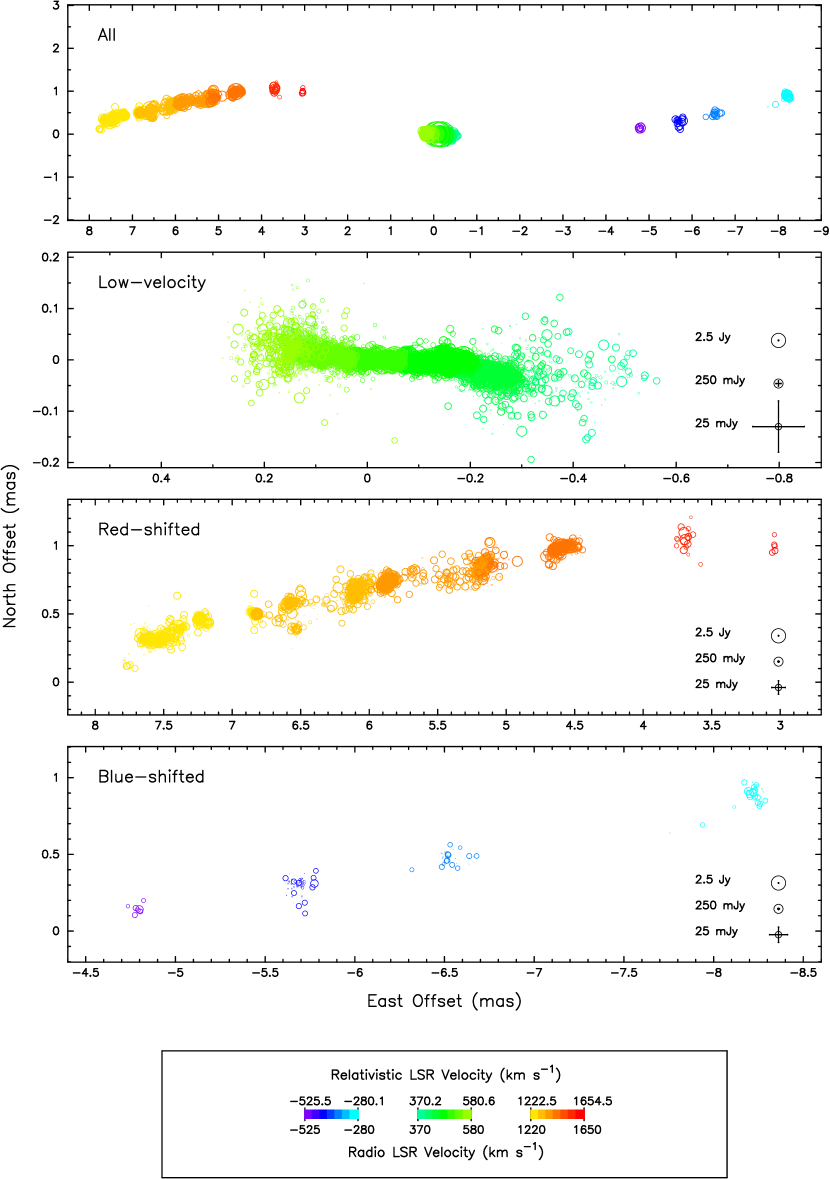
Figure 6: Maps of maser emission for all epochs superposed. (top) The full velocity range of the emission. (upper middle) Low-velocity emission. (lower middle) Red-shifted high-velocity emission. (bottom) Blue-shifted high-velocity emission. Symbol diameter is proportional to the logarithm of peak flux density. Each panel is scaled separately. A key on the right hand side of the three lower panels gives the symbol sizes of 2.5 Jy, 250 mJy, and 25 mJy masers, as well as the x-y sizes of their associated random errors. The color bar at bottom codes nonrelativistic LSR velocity (lower label) or relativistic LSR velocity (upper label). Note that the thinness of the maser disk in the low-velocity panel is obscured by the large number of masers plotted. See Figures 7-9 for additional discussion.

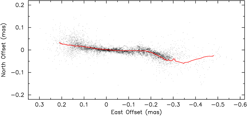
Figure 7: Map of low-velocity maser emission. All masers have the same symbol size. The red curve is the boxcar smoothed (30 km s^-1 width) weighted average of low-velocity masers, computed from medium-sensitivity epochs (see $\S 3.2$).

Maser Maps — We present the full set of Gaussian fits for detected maser spots in Table 5. Note that spots that lie in the overlap between adjacent basebands appear twice. Quoted position uncertainties are fitted random error. The true random error is estimated to be the maximum of the fitted random error and the random error computed according to Table 4. The sky distribution and related statistics of the masers are shown in Figures 6-9; the position along the major axis of the disk versus LSR velocity are shown in Figures 10-13. We define the impact parameter to be $b=\pm(\Delta x^{2}+\Delta y^{2})^{1/2},$ where $\Delta x$ and $\Delta y$ are the east-west and north-south offsets from the emission at 510.0 km s^-1 (relativistic), respectively, and the sign of b is taken from the sign of $\Delta x$ (which is feasible because the disk is elongated chiefly east-west). The formal uncertainty in impact parameter ($\sigma_{b}$) is given by

$$\sigma_{b}=\Bigl{[}\ {{(\Delta x\ \sigma_{x})^{2}+(\Delta y\ \sigma_{y})^{2}}\over{\Delta x^{2}+\Delta y^{2}}}\ \Bigr{]}^{1/2},$$

where $\sigma_{x}$ and $\sigma_{y}$ are the random components of uncertainty in east and north offsets, respectively.

Continuum Maps — We detected continuum emission $>3\sigma$ in fifteen epochs and averaged deconvolved images (with uniform weighting) to obtain a peak intensity of 1.1 mJy ($23\sigma$) (Figure 14). Nondetection for the remaining three epochs may be attributed to known time variability of the source (Herrnstein et al., 1998). In Table 6, we list (angle integrated) flux densities and centroid positions. Figure 15 shows a plot of flux density versus time. Our measurements are consistent with the hypothesis that the emission traces a jet extending outward from the central engine, along the spin axis of the accretion disk (Herrnstein et al., 1998).

3.2 Position Shifts

Visual comparison shows that the position-velocity loci for low- and red-shifted high-velocity emission are offset at a few epochs by up to $\sim 30\mu$as from a weighted average locus computed from the medium-sensitivity epochs. The shifts do not appear to be frequency dependent. We attribute them to residual phase offsets between basebands correlated in separate passes (as were low and high-velocity bands), uncertainty in the post self-calibration registration that was required for particular high-sensitivity epochs, and unmodeled changes in the structure of the reference emission from epoch to epoch.

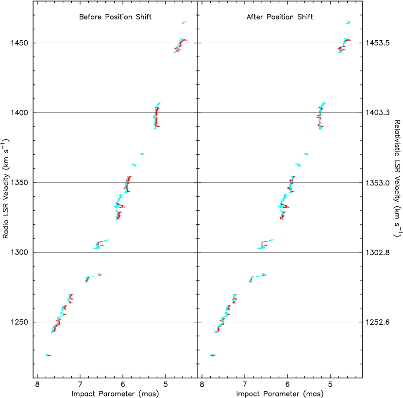
Figure 16: Position–velocity traces for red-shifted emission that demonstrate the magnitude of the postion offset affecting some epochs and the effectiveness of correction ($\S 3.2$). Both panels show the weighted average of red-shifted masers in medium-sensitivity epochs (blue) and the trace for one high-sensitivity observation, BM112H (red). (left) – No position shift to the BM112H data is applied. The masers appear to be offset in position from the weighted average. (right) – Good agreement after a single position shift (applied to the BM112H data) that minimizes the offset in a least squares sense.

We computed corrections for this effect as follows. First, we constructed variance-weighted average x and y positions for each channel from all medium-sensitivity epochs. (Weighting depended upon random measurement error alone.) Next, we downweighted outliers according to the empirical scheme below and computed new variance-weighted averages. To downweight outlying samples, we multiplied measurement errors by an empirical factor that increased with offset: $\exp({\Delta\over 4\sigma})^{2}$, where $\Delta$ is the offset in $x$ or $y$ from the weighted average and $\sigma$ is the unmodified measurement uncertainty. For instance, the measurement error for points that deviated by $6\sigma$ is increased by a factor of 10, whereas the measurement error for points that deviated by $1\sigma$ is increased by a factor of 1.06. Finally, we obtained offset corrections for individual epochs (both high- and medium-sensitivity) by minimizing the sum of the squares of the offsets from the variance-weighted averages above. Figure 16 shows the observed and corrected offsets for red-shifted emission in observation BM112H, an epoch with one of the largest shifts. Table 7 quantifies the computed shifts for each epoch, which we applied to the data. However, we note that Table 5 contains uncorrected maser spot positions. In addition, no corrections have been computed for blue-shifted emission because it is too sparse to enable comparisons.

4 The Sky Distribution of Maser Emission

Maser emission in NGC 4258 traces a thin, slightly warped, nearly edge-on disk (Miyoshi et al., 1995; Herrnstein et al., 1998, 2005). The new VLBI data (Figure 6) trace this structure more fully, due to both emission time variability (i.e., development of new Doppler components) and broader observing bandwidth (e.g., velocities above 1500 km s^-1). The flaring (in north offset range) of low-velocity maser spots at the east offset edges of the plot is an artifact and is due to the fact that the weaker spots, which have lower positional accuracy, are preferentially located away from the middle of the low-velocity spectrum (Figure 1). Crowding of plot symbols also obscures the relative breadths of the distributions of maser spots with different flux densities. To assess the statistics of the distribution of maser spots, we have computed perpendicular offsets of low-velocity masers from a boxcar-smoothed (30 km s^-1 width), weighted average locus of emission observed in the medium-sensitivity epochs. For spots $<250$ mJy, the distribution is Gaussian and is consistent with measurement noise (Figure 8, top panel). For spots $>250$ mJy, the distribution exhibits significant non-Gaussian wings and tail (Figure 8, bottom panel), which is a result of source structure on scales of order 10 $\mu$as. If we restrict the velocity range under consideration, the distribution of strong spots may be related to accretion disk thickness. The inclination and position angle warp of the disk combine to create a concavity on the near side, the bottom of which is tangent to our line of sight (i.e., the disk is seen edge-on at this point). Maser spots in the velocity range 485-510 km s^-1 lie in this part of the disk (Herrnstein et al., 2005, their Figure 14). Previously measured accelerations for masers in this velocity range are 8-10 km s^-1 yr^-1, which suggests a radius of 3.7-4.1 mas and from the warp model we infer a projected range vertical offset of only 3 $\mu$as. The observed distribution of maser spot position offsets from the mean locus is nearly Gaussian with $\sigma$ = 5.1 $\mu$as (12 $\mu$as at full-width half-maximum). Because most of the maser spot positions in this velocity range are measured with $<3\mu$as accuracy, we propose that this Gaussian distribution largely represents a true distribution about the local midplane of the disk (i.e., the thickness of warm molecular material.) See next section for interpretation.

5 Notes on Source Structure and Evolution

The long-term importance of VLBI monitoring of the NGC 4258 H₂O maser includes contributions to estimation of a geometric distance and its application to high-accuracy measurement of the Hubble constant. Estimation of a distance requires additional quantification of centripetal accelerations for disk material and modeling of 3-D disk structure and dynamics. These will be treated in follow-on papers. However, we can make several observations based on the time-series VLBI data alone.

Accretion disk thickness.— In prior analyses, scatter in low-velocity maser spot positions (north-south) have been used to estimate an upper limit on the thickness of the underlying accretion disk. Moran et al. (1995) obtained a limit of $\sim 10\mu$as by focusing on strong maser features toward the middle of the spectrum for a VLBI epoch in 1994. We have combined the results for all 18 VLBI epochs to obtain a time-average sample of emission for which the width of the distribution ($1\sigma$) is $5.1\mu$as. This may be the first directly measured thickness for an accretion disk around any black hole. In hydrostatic equilibrium the accretion disk is expected to have a Gaussian distribution of density as a function of height with $\sigma=r\ c_{s}/v_{\phi}$, where $r$ is the radius, $v_{\phi}$ is the orbital velocity, and $c_{s}$ is the sound speed (Frank, King, & Raine, 2002). Note that $v_{\phi}/r=(GM/r^{3})^{1/2}=\omega$, which is the slope of the impact parameter versus velocity curve of Figure 10 and equals $2.67\times 10^{-10}$ s^-1. Hence, for $\sigma=5.1\ \mu$as or $5.5\times 10^{14}$ cm, we obtain $c_{s}=1.5$ km s^-1, corresponding to a temperature of about 600 K (about half the limit given by Moran et al. (1995)). This temperature is consistent with the 400-1000 K range that is believed necessary for maser action from H₂O (Elitzur, 1992). Furthermore, the inferred sound speed is comparable to the line width of individual maser Doppler components seen in spectra, which is consistent with maser saturation. We note that in our discussion, we have assumed that the maser distribution samples the full thickness of the accretion disk, rather than a surface layer, whose depth could be well below that of the physical disk. This assumption is consistent with the disk models of Neufeld & Maloney (1995) for radiatively efficient accretion. A more detailed inspection of residuals from models fit to maser spot distributions (e.g., residuals arising from an antisymmetric offset perpendicular to the disk plane, caused by irradiation of “upper” and “lower” surfaces of the disk for high-velocity red- and blue-shifted masers) is necessary for further comment. We also note that the measured thickness places a limit on the magnetic pressure. The magnetic field strength must be less than about 100 mG, which is about the current limit from the non detection of the Zeeman effect (Modjaz et al., 2005).

Highly red-shifted emission.— Red-shifted emission at velocities $\gg 1460$ km s^-1 has been mapped here for the first time. Emission at 1647 km s^-1 was first reported by Modjaz et al. (2005) in a single-dish spectrum, while the 1566 km s^-1 Doppler component was previously unknown. The detection of these very high velocity emissions enables the mid-line of the disk, along which the rotation curve is apparent, to be traced to about 30% smaller radii ($\approx 0.11$ pc) than before. This innermost radius is now also $\approx 20\%$ smaller than that for the low-velocity emission. Perhaps most importantly, the radius of the 1647 km s^-1 emission is small enough that curvature in the disk is directly observable, which will enble more robust geometric modeling of the warp (cf. Miyoshi et al., 1995; Herrnstein et al., 1998).

The low-velocity emission was shown by Herrnstein et al. (2005) to originate near the bottom of a concave depression on the near side of the disk, where our line of sight is tangent to the disk. We note that in contrast, the 1566 km s^-1 component lies near the topmost portion of the spine of the disk projected on the sky. For an “alien” observer viewing the disk edge-on along a line of sight close to our sky plane, the material we perceive at 1566 km s^-1 would probably be responsible for strong low-velocity emission. Conceivably, the intensity of that emission would be boosted by seed photons from the northern lobe of the radio jet, much as the low-velocity emission visible to earthbound observers is believed to be boosted by the southern lobe of the jet (Herrnstein et al., 1997). The resulting (competitive) beaming of maser energy along a radial path may be responsible for the low intensity of the 1566 km s^-1 emission, for which the dominant gain path is orthogonal.

Source Symmetry.— Early VLBI maps of the maser emission exhibited asymmetry, wherein the blue-shifted high-velocity emission spanned a truncated range of radii compared to red-shifted emission (Miyoshi et al., 1995). It was unclear whether this was a reflection of limited sensitivity (since the blue-shifted emission is quite weak) or a ramification of unmodeled disk structure. Detection of emission over a broader range of radius (i.e., velocity) has been accomplished since then. Nakai et al. (1995) first observed a broader range via single-dish spectroscopy, detecting emission near $-300$ and $-500$ km s^-1 one time each, in $\approx 20$ epochs spaced over $\approx 200$ days. In their Figure 3, Herrnstein et al. (2005) also show data derived from a VLBI detection of blue-shifted emission near $-300$ and $-500$ km s^-1 at one epoch in 1996 September. With new detections shown in our Figure 13 at $\approx-285$ km s^-1 (7 epochs over 2-3 years) and $\approx-515$ km s^-1 (2 epochs over 8 days), we confirm the distribution of blue-shifted high-velocity emission over a $\approx 0.1$ pc range of radius. In light of the very high velocity red-shifted emission reported here (which shows that warm molecular material extends to relatively small radii), and assuming mirror symmetry of the maser disk, we hypothesize there may be still higher velocity blue-shifted emission that could be detected in the vicinity of $-600$ km s^-1. However, any such emission is likely to be weak, perhaps on the order of 1 mJy, based on line ratios among known Doppler components.

Envelope of low-velocity emission.—Our long term monitoring of velocities between the high and low-velocity emission complexes has not resulted in detected intermediate-velocity emission. Nondetection here and in episodic single-dish spectroscopy of comparable sensitivity (e.g., Modjaz et al., 2005) may exclude the possibility of long gain paths at disk azimuth angles more than $\approx 0.1$ rad from the emission close to the systemic velocity. This contrasts with what has been found in the NGC 1068 H₂O maser (Greenhill & Gwinn, 1997), wherein the locus of “low-velocity” maser emission extends in a ring over a full quadrant on the receding side of the disk. However, in the angular extent of high brightness temperature continuum emission that can provide seed photons for amplification differs. In NGC 4258, they arise from a compact jet core (Herrnstein et al., 1997, 2005), while in NGC 1068, they are believed to arise from an extended region that more or less fills the volume inside the innermost maser orbit (Gallimore et al., 2001)–though the absence of seeded emission in the adjacent (approaching) quadrant is difficult to explain.

Though centripetal acceleration is responsible for the observed secular drift of individual Doppler component velocities, the overall range of emission does not change discernably in angle or velocity. In our time monitoring, we detected low-velocity emission from $\approx 380$ to 580 km s^-1. This range is comparable to the ranges observed in high-sensitivity spectroscopic studies over the period 1992-2005 (e.g., Greenhill et al., 1995b; Nakai et al., 1995; Yamauchi et al., 2005; Modjaz et al., 2005). Any secular change of the upper and lower limits of the envelope appears to be much smaller than the 10 km s^-1 yr^-1 drift of individual Doppler components.

No maser spots seen away from the disk.—In contrast to maser emission from the Circinus galaxy (Greenhill et al., 2003) and NGC 1068 (Gallimore et al., 1996, 2001), we found no Doppler components more than a beamwidth ($\approx$ 1 mas) from the locus of disk emission. Our detection limit was 13 mJy ($6\sigma$) for the highest sensitivity observation, BM112H. In Circinus, the maser population not associated with the disk is believed to trace a bipolar, wide-angle outflow that contains clumps moving away from the central engine, at radii as small as $\approx 0.1$ pc. In NGC 1068, the non-disk emission lies $\gg 1$ pc downstream in the narrow-line region, along the jet axis. The absence of emission associated with wind or jet emission in NGC 4258 (see $\S 2.4$) may be a consequence of a lower luminosity central engine and more tightly bound disk material (i.e., smaller disk mass compared to the central engine mass).

Absorption signatures.—Watson & Wallin (1994) hypothesized that thermalized water molecules in disks could absorb maser emission arising at smaller radii; the observational signature would be troughs in spectra near systemic velocities. A number of spectra for NGC 4258 that are in the literature do exhibit dips in the vicinity of the systemic velocity, including time averages of many spectra collected over periods of months or years (see Bragg et al., 2000, and references therein, as well as our Figures 1,5). The cumulative record of VLBI observations does not demonstrate notable structure in the vicinity of the systemic velocity, which is consistent with expectations. However, evidence thus far has been anecdotal (e.g., compare spectra for epochs 2000.08 and 2000.61). Systematic analysis of spectra obtained throughout 1985 and 1986 demonstrated that troughs in spectra exhibited secular drift similar to that of neighboring emission components (Greenhill et al., 1995b). A physical model of the NGC 4258 warped accretion disk presents additional hurdles to the hypothesis. In the case of NGC 4258, the vertical deviation of the disk from a plane displaces material at large radii from the line of sight (Herrnstein et al., 2005), and the velocity at which the longest coherence lengths occur (overlapping the rest frame transitions of inverted and thermalized material) is displaced $\sim 20$ km s^-1 redward from the systemic velocity. Moreover, the model of Neufeld & Maloney (1995) predicts that material at sufficiently large radii is atomic, and thus cannot form an absorbing layer.

6 Conclusion

We have reported a four year time-series VLBI study of the H₂O maser in NGC 4258, with quadruple the number of epochs than earlier work. Overall source structure during the four years of our study resembled what has previously been fitted to an inclined, warped, Keplerian disk model. Frequent sampling over years enabled compilation of a more complete census of time variable Doppler components and broad observing bandwidth enabled detection and mapping of material with larger orbital velocities than before. The persistence and symmetry of source structure is now more clear, and the accuracy of position measurement has been improved. Detailed analysis of the distribution of maser spots perpendicular to the local disk plane, interpreted in the context of hydrostatic support, suggests a disk thickness ($\sigma$ = $5.5\times 10^{14}$ cm) and gas temperature of about 600 K. The new catalog of maser spot positions and line-of-sight velocities will enable construction of a more robust (3-D) dynamical disk model and more accurate measurement of maser centripetal acceleration and proper motion. Together, these will enable estimation of a geometric distance with smaller random and systematic uncertainty (cf. Herrnstein et al., 1999). Follow-up papers will treat the measurement of acceleration, modeling, and comparison of a final “maser distance” to a new four-color Cepheid distance that enables recalibration of distance indicators and ultimately H_∘.

Table 1: The Observations

Experiment Code	Date	Antennas	Synthesized Beam	Sensitivity	Coverage			Comments
			(mas$\times$mas, deg)	(mJy)
					L	R	B
BM056C	1997 March 06 (1997.18)	VLBA, VLA, EFLS	0.65$\times$0.53, $+$12.5	3.0	x	x	x
BM081A	1997 October 01 (1997.75)	VLBA, VLA, EFLS	0.59$\times$0.35, 1$-$7.2	2.7	x	x	x
BM081B	1998 January 27 (1998.07)	VLBA, VLA, EFLS	0.60$\times$0.42, 1$+$5.1	3.2	x	x	x
BM112A	1998 September 05 (1998.68)	VLBA, VLA, EFLS	0.67$\times$0.49, 1$+$8.5	3.0	x	x	x
BM112B	1998 October 18 (1998.80)	VLBA	0.52$\times$0.36, $-$18.0	4.2	x	x
BM112C	1998 November 16 (1998.88)	VLBA	0.53$\times$0.35, $-$14.9	4.0	x		x
BM112D	1998 December 24	VLBA			x	x		miscorrelated
BM112E	1999 January 28 (1999.08)	VLBA	0.51$\times$0.34, 1$-$6.0	4.4	x		x
BM112F	1999 March 19 (1999.21)	VLBA	0.48$\times$0.34, $-$10.0	4.1	x	x
BM112G	1999 May 18 (1999.38)	VLBA	0.50$\times$0.35, $-$10.8	4.8	x		x
BM112H	1999 May 26 (1999.40)	VLBA, VLA, EFLS	0.43$\times$0.26, $-$31.3	2.3	x	x	x
BM112I	1999 July 15	VLBA			x	x		corrupted
BM112J	1999 September 15 (1999.71)	VLBA	0.51$\times$0.32, 1$-$5.4	5.8	x		x
BM112K	1999 October 29 (1999.83)	VLBA	0.50$\times$0.34, $-$19.2	4.3	x	x
BM112L	2000 January 07 (2000.02)	VLBA	0.50$\times$0.34, $-$12.0	3.6	x		x
BM112M	2000 January 30 (2000.08)	VLBA	1.25$\times$0.35, $+$38.8	4.3	x	x
BM112N	2000 March 04 (2000.17)	VLBA	0.48$\times$0.33, $-$10.9	3.9	x		x
BM112O	2000 April 12 (2000.28)	VLBA	0.63$\times$0.37, $-$24.4	5.0	x	x
BM112P	2000 May 04 (2000.34)	VLBA	0.50$\times$0.34, $-$11.4	4.6	x		x
BG107	2000 August 12 (2000.61)	VLBA, VLA, EFLS	0.46$\times$0.36, $-$14.3	4.7	x	x	x

Table 2: Instrument Setup

Experiment Code	Bandwidth	Emission Type	Bandpass	Band center vLSR	Tuning of Bandpass
	(MHz)			(km s-1)
BM056C; BM081A,B; BM112A,H	18	low-velocity	11	618.89	LCP
			12	533.95	LCP
			13	511.24	LCP
			14	426.30	LCP
		red-shifted	15	1447.41	RCP
			16	1359.37	RCP
			17	1339.76	RCP
			18	1251.72	RCP
		blue-shifted	19	$-$336.09	RCP
			10	$-$424.00	RCP
			11	$-$443.74	RCP
			12	$-$531.65	RCP
BG107	18	low-velocity	11	665.00	LCP
			12	580.00	LCP
			13	495.00	LCP
			14	410.00	LCP
		red-shifted	15	1485.00	RCP
			16	1400.00	RCP
			17	1315.00	RCP
			18	1230.00	RCP
		blue-shifted	19	$-$255.00	RCP
			10	$-$340.00	RCP
			11	$-$425.00	RCP
			12	$-$510.00	RCP
BM112B,F,K,M,O	16	low-velocity	11	836.00	LCP
			12	653.00	LCP
			13	470.00	RCP
			14	470.00	LCP
		red-shifted	15	1568.00	LCP
			16	1385.00	LCP
			17	1202.00	LCP
			18	1019.00	LCP
BM112C,E,G,J,L,N,P	16	low velocity	11	500.00	RCP
			12	500.00	LCP
			13	317.00	LCP
			14	134.00	LCP
		blue-shifted	15	$-$49.00	LCP
			16	$-$232.00	LCP
			17	$-$415.00	LCP
			18	$-$598.00	LCP

Table 3: Station Positions and Velocities

Station	Station Position			Error
	X	Y	Z	X	Y	Z
	(m)	(m)	(m)	(cm)	(cm)	(cm)
VLBA-BR	$-$2112064.9661	$-$3705356.5115	4726813.7932	0.0476	0.0885	0.1069
EFLS	$-$4033947.4792	486990.5244	4900430.8031	0.2577	0.0669	0.3094
VLBA-FD	$-$1324009.1202	$-$5332181.9713	3231962.4738	0.0327	0.1031	0.0731
VLBA-HN	$-$1446375.1259	$-$4447939.6532	4322306.1181	0.0395	0.1275	0.1237
VLBA-KP	$-$1995678.6199	$-$5037317.7147	3357328.1296	0.0453	0.1104	0.0832
VLBA-LA	$-$1449752.3520	$-$4975298.5907	3709123.9270	0.0290	0.0830	0.0689
VLBA-MK	$-$5464074.9591	$-$2495249.1189	2148296.8444	0.1700	0.1071	0.1037
VLBA-NL	$-$130872.2452	$-$4762317.1215	4226851.0426	0.0217	0.1067	0.0953
VLBA-OV	$-$2409150.1035	$-$4478573.2283	3838617.3949	0.0546	0.1027	0.0919
VLBA-PT	$-$1640953.7026	$-$5014816.0276	3575411.8817	0.0321	0.0851	0.0692
VLBA-SC	$-$2607848.5236	$-$5488069.6773	1932739.5281	0.1088	0.2388	0.1104
VLA	$-$1601185.2077	$-$5041977.1729	3554875.7033	$\approx 1.0$	$\approx 1.0$	$\approx 1.0$
Station	Station Velocity			Error
	X	Y	Z	X	Y	Z
	(cm yr-1)	(cm yr-1)	(cm yr-1)	(cm yr-1)	(cm yr-1)	(cm yr-1)
VLBA-BR	$-$1.2800	$-$0.0370	$-$1.1200	0.0160	0.0280	0.0304
EFLS	$-$1.5250	$-$1.7100	$-$0.8950	0.0492	0.0184	0.0626
VLBA-FD	$-$1.1600	$-$0.2380	$-$0.7040	0.0102	0.0234	0.0194
VLBA-HN	$-$1.4430	$-$0.1430	$-$0.0850	0.0142	0.0436	0.0387
VLBA-KP	$-$1.2210	$-$0.0150	$-$0.9740	0.0149	0.0309	0.0255
VLBA-LA	$-$1.2850	$-$0.0170	$-$0.8300	0.0083	0.0174	0.0165
VLBA-MK	$-$1.3600	$-$6.0080	$-$2.9420	0.0547	0.0428	0.0427
VLBA-NL	$-$1.4180	$-$0.0090	$-$0.4710	0.0095	0.0289	0.0245
VLBA-OV	$-$1.6270	$-$0.5910	$-$0.8200	0.0169	0.0305	0.0268
VLBA-PT	$-$1.3610	$-$0.2480	$-$0.8590	0.0073	0.0147	0.0151
VLBA-SC	$-$0.9840	$-$0.4390	$-$1.0200	0.0331	0.0784	0.0445
VLA	$-$1.3140	$-$0.1100	$-$0.8560	$\approx 0.1$	$\ \,\approx 0.1$	$\approx 0.1$

Table 4: Largest Sources of Relative Position Error in Synthesis Maps

Type of Error	Magnitude over 75 MHz	Magnitude over 4 MHz	Comments
	($\mu$as)	($\mu$as)
Random	1	1	1 Jy peak (strong)
	255	255	50 mJy peak (weak)
Systematic (full frequency range):
Positional Uncertainty of Reference Feature	105	$<$ 115	Uncertainty in absolute position of reference feature:
			$\alpha=0{\hbox to0.0pt{.\hss}}^{s}\!0003,\,\delta=0{\hbox to0.0pt{.\hss}}{{}^{\prime\prime}}\!003$
Atmospheric Delay Error	6	$<$ 115
Frequency Standard Uncertainty	2	$<$ 115
Positional Uncertainty of Calibrator	1	$<$ 115	Uncertainty in absolute position of calibrators:
			$\alpha=0{\hbox to0.0pt{.\hss}}^{s}\!000042,\,\delta=0{\hbox to0.0pt{.\hss}}{{}^{\prime\prime}}\!00047$ ( 4C39.25 ),
			$\alpha=0{\hbox to0.0pt{.\hss}}^{s}\!000114,\,\delta=0{\hbox to0.0pt{.\hss}}{{}^{\prime\prime}}\!00027$ (1150$+$81),
			$\alpha=0{\hbox to0.0pt{.\hss}}^{s}\!000020,\,\delta=0{\hbox to0.0pt{.\hss}}{{}^{\prime\prime}}\!00026$ (1308$+$33)
Baseline Coordinate Uncertainty	1	$<$ 115
Systematic (relative frequencies):
Clock Uncertainty	…	2

Table 5: Channel Data

channel	$v_{\rm LSR}$	$v_{\rm rel}$	Fν	$\sigma_{{\rm F}_{\nu}}$	$\Delta x$	$\sigma_{x}$	$\Delta y$	$\sigma_{y}$	maj	$\sigma_{\rm maj}$	min	$\sigma_{\rm min}$	pa	$\sigma_{\rm pa}$	$v_{\rm band}$
(1$-$512)	(km s-1)	(km s-1)	(Jy)	(mJy)	(mas)	(mas)	(mas)	(mas)	(mas)	(mas)	(mas)	(mas)	(∘)	(∘)	(km s-1)
177	1464.157	1467.702	0.038	3.690	4.458	0.024	0.784	0.032	0.82	0.08	0.57	0.05	167	10	1447.41
178	1463.946	1467.490	0.054	3.850	4.486	0.018	0.783	0.023	0.71	0.05	0.53	0.04	7	10	1447.41
179	1463.735	1467.279	0.057	3.770	4.499	0.017	0.750	0.022	0.71	0.05	0.54	0.04	19	9	1447.41
180	1463.525	1467.067	0.044	3.680	4.508	0.021	0.753	0.028	0.68	0.06	0.60	0.05	23	27	1447.41
223	1454.466	1457.964	0.027	3.570	4.475	0.033	0.778	0.043	0.71	0.09	0.42	0.06	12	10	1447.41
224	1454.255	1457.752	0.039	3.550	4.503	0.023	0.791	0.030	0.65	0.06	0.49	0.04	14	13	1447.41
225	1454.045	1457.541	0.057	3.560	4.531	0.016	0.776	0.020	0.65	0.04	0.55	0.03	14	15	1447.41
226	1453.834	1457.329	0.079	3.620	4.523	0.012	0.782	0.015	0.68	0.03	0.55	0.03	24	8	1447.41
227	1453.623	1457.117	0.092	3.730	4.513	0.010	0.800	0.013	0.71	0.03	0.55	0.02	15	6	1447.41
228	1453.413	1456.906	0.102	3.720	4.512	0.009	0.814	0.012	0.69	0.03	0.55	0.02	9	6	1447.41
229	1453.202	1456.694	0.106	3.620	4.515	0.009	0.802	0.011	0.68	0.02	0.53	0.02	8	5	1447.41
230	1452.991	1456.482	0.112	3.610	4.517	0.008	0.803	0.011	0.65	0.02	0.52	0.02	8	6	1447.41
231	1452.781	1456.271	0.114	3.560	4.515	0.008	0.818	0.010	0.65	0.02	0.54	0.02	6	6	1447.41
232	1452.570	1456.059	0.115	3.680	4.538	0.008	0.823	0.011	0.66	0.02	0.55	0.02	17	7	1447.41
233	1452.359	1455.847	0.116	3.680	4.546	0.008	0.821	0.010	0.69	0.02	0.52	0.02	9	4	1447.41

Note. — Table 5 provides the Channel data for all the observations and is published in its entirety in the electronic edition of the Astrophysical Journal. A portion is shown here for guidance regarding its form and content.

Table 6: Continuum Detections

Epoch	Freq.	Fν	rms	$\Delta x$	$\sigma_{x}$	$\Delta y$	$\sigma_{y}$
		(mJy)	(mJy)	(mas)	(mas)	(mas)	(mas)
BM056C	blue-shifted	$<$ 1.19	0.18	$-$0.240	0.051	0.952	0.055
BM081B	red-shifted	$<$ 1.66	0.19	$-$0.108	0.022	0.800	0.032
	blue-shifted	$<$ 1.28	0.19	$-$0.194	0.028	1.018	0.035
BM112B	red-shifted	$<$ 1.53	0.19	$-$0.007	0.037	1.360	0.099
BM112C	blue-shifted	$<$ 1.67	0.18	$-$0.190	0.028	1.099	0.070
BM112E	blue-shifted	$<$ 2.40	0.20	$-$0.028	0.030	0.952	0.048
BM112F	red-shifted	$<$ 1.90	0.19	$-$0.039	0.054	0.897	0.093
BM112G	blue-shifted	$<$ 0.72	0.21	$-$0.200	0.047	1.008	0.080
BM112J	blue-shifted	$<$ 1.70	0.26	$-$0.147	0.075	1.093	0.147
BM112K	red-shifted	$<$ 1.72	0.19	$-$0.192	0.134	1.534	0.213
BM112L	blue-shifted	$<$ 1.75	0.16	$-$0.009	0.029	1.252	0.061
BM112M	red-shifted	$<$ 2.68	0.20	$-$0.346	0.363	0.990	0.157
BM112N	blue-shifted	$<$ 2.39	0.18	$-$0.049	0.013	0.871	0.030
BM112O	red-shifted	$<$ 4.01	0.24	$-$0.022	0.021	0.947	0.040
BM112P	blue-shifted	$<$ 2.52	0.21	$-$0.029	0.061	1.018	0.077
BG107	red-shifted	$<$ 3.95	0.22	$-$0.133	0.015	1.050	0.018
	blue-shifted	$<$ 3.66	0.20	$-$0.152	0.010	1.022	0.013

Table 7: Derived Position Shifts

Experiment Code	Low-velocity Masers				Red-shifted Masers
	x	$\sigma_{x}$	y	$\sigma_{y}$	x	$\sigma_{x}$	y	$\sigma_{y}$
	($\mu$as)	($\mu$as)	($\mu$as)	($\mu$as)	($\mu$as)	($\mu$as)	($\mu$as)	($\mu$as)
BM056C	$-$8	3	$-$1	4	$-$5	5	$-$1	6
BM081A	$-$5	1	$-$3	2	$-$8	4	$-$10	6
BM081B	$-$4	2	$-$11	2	$-$1	3	$-$3	5
BM112A	$-$8	2	$-$3	4	$-$33	5	$-$6	8
BM112B	$-$5	3	$-$0	5	$-$ 2	5	$-$0	7
BM112C	$-$3	2	$-$2	3
BM112E	$-$0	3	$-$1	4
BM112F	$-$4	2	$-$2	3	$-$3	4	$-$6	6
BM112G	$-$3	3	$-$8	4
BM112H	$-$6	1	$-$0	2	$-$24	4	$-$0	6
BM112J	10	3	$-$6	4
BM112K	$-$1	2	$-$1	3	$-$5	6	$-$3	8
BM112L	$-$3	2	$-$3	3
BM112M	$-$7	3	$-$5	10	$-$5	4	$-$0	14
BM112N	$-$3	3	$-$6	4
BM112O	$-$7	4	$-$9	6	$-$12	4	$-$15	7
BM112P	$-$2	3	$-$10	4
BG107	$-$20	4	$-$0	5	$-$17	7	$-$37	9

Figure 1: Spectra for low-velocity masers. The vertical scale on the page is the same for each plot. The spectra show the total imaged power obtained from the fitted peak flux densities of maser spots. Channels with no detectable emission are not shown. Velocities are defined with respect to the Local Standard of Rest, assuming the nonrelativistic radio definition of Doppler shift (bottom axis) and relativistic radio definition of Doppler shift (top axis).

Figure 2: Spectra for red-shifted masers, displayed as in Figure 1. The Doppler components at 1566 km s^-1 (epochs 1999.21, 1999.83, and 2000.08) and 1647 km s^-1 (epochs 1999.83, 2000.08, and 2000.28) are shown separately in Figure 3.

Figure 3: Spectra for red-shifted masers at 1566 km s^-1 and 1647 km s^-1, displayed as in Figure 1. The dotted portions of the spectra delineate fits that fall below our $6\sigma$ threshold (see text for details).

Figure 4: Spectra for blue-shifted masers, displayed as in Figure 1. The dotted portions of the spectra delineate fits that fall below our $6\sigma$ detection threshold (see text for details).

Figure 5: Unweighted average maser spectra for all observing epochs (1997-2000), displayed as in Figure 1. (top) Low-velocity emission. (middle) Red-shifted high-velocity emission. (bottom) Blue-shifted high-velocity emission. LSR velocities are defined assuming the nonrelativistic radio definition of Doppler shift (bottom axis) or relativistic radio definition of Doppler shift (top axis).

Figure 8: Histograms of separations between individual low-velocity maser spots and the average emission locus (Figure 7, red curve). Each offset is divided by the corresponding random measurement uncertainty. All low-velocity masers are plotted. (top) Low-velocity masers $<250$ mJy, for which corresponding measurement uncertainties are $>5\mu$as, plotted. The distribution for weak masers is Gaussian (see superposed curve), as would be expected from a noise dominated distribution. (bottom) Low-velocity masers $>250$ mJy, for which corresponding measurement uncertainties are $<5\mu$as, plotted. The distribution for strong masers exhibits nonGaussian wings and tail (see superposed curve) that may be attributed to source structure or systematic error arising from the representation of the disk plane position by the average of maser spot positions (Figure 7, red curve), at the few $\mu$as level.

Figure 9: Histogram as in Figure 8 for masers $>250$ mJy but for the velocity range $485-510$ km s^-1 (East Offset $-0.1$ to $0.0$ mas). This is the velocity range over which the model accretion disk (Herrnstein et al., 2005) is viewed edge-on. The distribution of strong masers is nearly Gaussian (see superposed curve) with full-width at half-maximum (FWHM) of $\approx 12\mu$as ($\sigma\approx 5.1\mu$as), which we interpret to be the underlying accretion disk thickness.

Figure 10: Position–velocity diagram for all epochs superposed. Positive impact parameters are to the east. The linear gradient in low-velocity emission is characteristic of emission from material in highly inclined circular orbits over a narrow range of radii. The fitted straight line marks the locus for emission at a single radius. (A steeper line indicates a smaller radius). High-velocity masers trace declining rotation curves, which are fitted here in position–velocity space and shown for Keplerian orbits. Good agreement with the model $v-v_{sys}\propto|b|^{-0.5}$, where $v_{sys}$ is systemic velocity and $b$ is impact parameter, suggests that the high-velocity emission arises close to a single diameter through the underlying disk and that warping is of second-order importance (e.g., Miyoshi et al., 1995). We note that the Doppler components at 1566 km s^-1 and 1647 km s^-1 appear to arise inside the mean radius of the low-velocity emission. Nothing has previously been mapped at these small radii. LSR velocities are defined assuming the nonrelativistic radio definition of Doppler shift (left-hand axis) or relativistic radio definition of Doppler shift (right-hand axis).

Figure 11: Position–velocity traces for low-velocity emission at each epoch individually. The impact parameter scale is shown in the bottom left corner of the figure and the separation between traces is proportional to the time between epochs (denoted by numeric labels). Horizontal error bars denote uncertainty in impact parameter and reflect random error only. LSR velocities are defined assuming the nonrelativistic radio definition of Doppler shift (left-hand axis) or relativistic radio definition of Doppler shift (right-hand axis).

Figure 12: Position–velocity traces for high-velocity red-shifted emission, plotted as in Figure 11. There are fewer traces here because red-shifted emission was only observed in alternate medium-sensitivity epochs (Table 1). Keplerian curves (see Figure 10) were drawn through the data of each epoch for ease of display.

Figure 13: Position–velocity traces for high-velocity blue-shifted emission, plotted as in Figure 11. There are fewer traces here because blue-shifted emission was only observed in alternate medium-sensitivity epochs (Table 1). Keplerian curves (see Figure 10) were drawn through the data of each epoch (circled) for ease of display.

Figure 14: Map of time-averaged continuum emission obtained from a uniformly weighted average of images from fifteen epochs. The rms noise level is 0.05 mJy. Contours are in $2.5\sigma$ steps, starting at $2.5\sigma$. An average restoring beam is shown in the lower right. The origin of coordinates is at the position of the maser reference feature.

Figure 15: Light curve of flux density for epochs with peak continuum emission $>3\sigma$ (see Table 6). Strictly speaking, this is not a total flux density, but rather an angle integrated flux density, since we measure it with an interferometer that has a limited range of baseline lengths.

References

- Benedict et al. (2002a) Benedict, G. F., et al. 2002a, AJ, 123, 473
- Benedict et al. (2002b) Benedict, G. F., et al. 2002b, AJ, 124, 1695
- Bragg et al. (2000) Bragg, A. E., Greenhill, L. J., Moran, J. M., & Henkel, C. 2000, ApJ, 535, 73
- Cecil, Wilson, & Tully (1992) Cecil, G., Wilson, A. S., & Tully, R. B. 1992, ApJ, 390, 365
- Claussen et al. (1984) Claussen, M. J., Heiligman, G. M., & Lo, K. Y. 1984, Nature, 310, 298
- Elitzur (1992) Elitzur, M. 1992, Astronomical Masers (Dordrecht: Kluwer Academic Publishers)
- Fiorentino et al. (2002) Fiorentino, G., Caputo, F., Marconi, M., & Musella, I. 2002, ApJ, 576, 402
- Fitzpatrick et al. (2002) Fitzpatrick, E. L., Ribas, I., Guinan, E. F., DeWard, L. E., Maloney, F. P., Massa, D. 2002, ApJ, 564, 260
- Fitzpatrick et al. (2003) Fitzpatrick, E. L., Ribas, I., Guinan, E. F., Maloney, F. P., Claret, A. 2003, ApJ, 587, 685
- Frank, King, & Raine (2002) Frank, J., King, A., & Raine, D. 2002, Accretion Power in Astrophysics (Cambridge: Cambridge University Press)
- Freedman et al. (2001) Freedman et al. 2001, ApJ, 553, 47
- Gallimore et al. (1996) Gallimore, J. F., Baum, S. A., O’Dea, C. P., Brinks, E., & Pedlar, A. 1996, ApJ, 462, 740
- Gallimore et al. (2001) Gallimore, J. F., Henkel, C., Baum, S. A., Glass, I. S., Claussen, M. J., Prieto, M. A., & Von Kap-herr, A. 2001, ApJ, 556, 694
- Greenhill et al. (1995a) Greenhill, L. J., Jiang, D. R., Moran, J. M., Claussen, M. J., & Lo, K. Y. 1995a, ApJ, 440, 619
- Greenhill & Gwinn (1997) Greenhill, L. J., & Gwinn, C. R. 1997, Ap&SS, 248, 261
- Greenhill et al. (1995b) Greenhill, L. J., Henkel, C., Becker, R., Wilson, T. L., & Wouterloot, J. G. A. 1995b, A&A, 304, 21
- Greenhill et al. (2003) Greenhill, L. J., et al. 2003, ApJ, 590, 162
- Groenewegen et al. (2004) Groenewegen, M. A. T., Romaniello, M., Primas, F., & Mottini, M. 2004, A&A, 420, 655
- Haschick, Baan, & Peng (1994) Haschick, A. D., Baan, W. A., & Peng, E. W. 1994, ApJ, 437, L35
- Herrnstein et al. (1997) Herrnstein, J. R., Moran, J. M., Greenhill, L. J., Diamond, P. J., Miyoshi, M., Nakai, N., & Inoue, M. 1997, ApJ, 475, L17
- Herrnstein et al. (1998) Herrnstein, J. R., Greenhill, L. J., Moran, J. M., Diamond, P.J., Inoue, M., Nakai, N., & Miyoshi, M. 1998, ApJ, 497, L69
- Herrnstein et al. (1999) Herrnstein, J. R., Moran, J. M., Greenhill, L. J., Diamond, P. J., Inoue, M., Nakai, N., Miyoshi, M., Henkel, C., & Riess, A. 1999, Nature, 400, 539
- Herrnstein et al. (2005) Herrnstein, J. R., Moran, J. M., Greenhill, L. J., & Trotter, A. S. 2005, ApJ, 629, 719
- Hu (2005) Hu, W. 2005, in “Observing Dark Energy,” eds. S. C. Wolff & T. R. Lauer, ASP Conf. Ser. 339, 215
- Humphreys et al. (2005) Humphreys, E. M. L., Argon, A. L., Greenhill, L. J., Moran, J. M., Reid, M. J. 2005, in Future Directions in High Resolution Astronomy: The 10th Anniversary of the VLBA, ASP Conference Proceedings, ed. Romney, J. D. & Reid, M. J. (San Francisco: Astronomical Society of the Pacific), 466
- Kennicutt et al. (1998) Kennicutt, R. C., et al. 1998, ApJ, 498, 181
- Kochanek (1997) Kochanek, C. S. 1997, ApJ, 491, 13
- Macri et al. (2007) Macri, L. M., Stanek, K. Z., Bersier, D. F., Greenhill, L. J., & Reid, M. J. 2007, ApJ, submitted
- Maoz & McKee (1998) Maoz, E. & McKee, C. F. 1998, ApJ, 494, 218
- Miyoshi et al. (1995) Miyoshi, M., Moran, J., Herrnstein, J., Greenhill, L., Nakai, N., Diamond, P., & Inoue, M. 1995, Nature, 373, 127
- Modjaz et al. (2005) Modjaz, M., Moran, J. M., Kondratko, P. T., & Greenhill, L. J. 2005, ApJ, 626, 104
- Moran et al. (1995) Moran, J., Greenhill, L., Herrnstein, J., Diamond, P., Miyoshi, M., Nakai, N., & Inoue, M. 1995, PNAS, 92, 11427
- Nakai, Inoue, & Miyoshi (1993) Nakai, N., Inoue, M., & Miyoshi, M. 1993, Nature, 361, 45
- Nakai et al. (1995) Nakai, N., Inoue, M., Miyazawa, K., Miyoshi, M., & Hall, P. 1995, PASJ, 47, 771
- Neufeld & Maloney (1995) Neufeld, D. A. & Maloney, P. R. 1995, ApJ, 447, L17
- Newman et al. (2001) Newman, J. A., et al. 2001, ApJ, 553, 562
- Nikolaev et al. (2004) Nikolaev, S., et al., 2004, ApJ, 601, 260
- Reid et al. (1988) Reid, M. J., Schneps, M. H., Moran, J. M., Gwinn, C. R., Genzel, R., Downes, D., & Rönnäng, B. 1988, ApJ, 330, 809
- Romaniello et al. (2006) Romaniello, M., Primas, F., Mottini, M., Groenewegen, M., Bono, G., & François, P. 2006, Memorie della Societa Astronomica Italiana, 77, 172
- Sakai et al. (2004) Sakai, S., Ferrarese, L., Kennicutt, R. C., & Saha, A. 2004, ApJ, 608, 42
- Sasselov et al. (1997) Sasselov, D. D., et al. 1997, A&A, 324, 471
- Spergel et al. (2006) Spergel, D. N., et al. 2006, ApJ, submitted (astro-ph/0603449)
- Thompson, Moran, & Swenson (2001) Thompson, A. R., Moran, J. M., & Swenson, G. W., Jr. 2001, Interferometry and Synthesis in Radio Astronomy (New York: Wiley-Interscience)
- van der Marel (2001) van der Marel, R. P. 2001, AJ, 122, 1827
- Watson & Wallin (1994) Watson, W. D. & Wallin, B. K. 1994, ApJ, 432, L35
- Yamauchi et al. (2005) Yamauchi, A., Sato, N., Hirota, A., & Nakai, N. 2005, PASJ, 57, 861