Error analysis in cross-correlation of sky maps:
application to the ISW detection

Abstract

Constraining cosmological parameters from measurements of the Integrated Sachs-Wolfe effect requires developing robust and accurate methods for computing statistical errors in the cross-correlation between maps. This paper presents a detailed comparison of such error estimation applied to the case of cross-correlation of Cosmic Microwave Background (CMB) and large-scale structure data. We compare theoretical models for error estimation with montecarlo simulations where both the galaxy and the CMB maps vary around a fiducial auto-correlation and cross-correlation model which agrees well with the current concordance $\Lambda$CDM cosmology. Our analysis compares estimators both in harmonic and configuration (or real) space, quantifies the accuracy of the error analysis and discuss the impact of partial sky survey area and the choice of input fiducial model on dark-energy constraints. We show that purely analytic approaches yield accurate errors even in surveys that cover only 10% of the sky and that parameter constraints strongly depend on the fiducial model employed. Alternatively, we discuss the advantages and limitations of error estimators that can be directly applied to data. In particular, we show that errors and covariances from the Jack-Knife method agree well with the theoretical approaches and simulations. We also introduce a novel method in real space that is computationally efficient and can be applied to real data and realistic survey geometries. Finally, we present a number of new findings and prescriptions that can be useful for analysis of real data and forecasts, and present a critical summary of the analyses done to date.

1 Introduction

The ISW effect (Sachs & Wolfe, 1967) has emerged as a new and powerful tool to probe our universe on the largest physical scales, testing deviations from General Relativity and the existence of dark-energy independent of other classical probes (e.g, Crittenden and Turok 1996; Bean and Dore 2004; Lue et al 2004; Cooray et al. 2004; Garriga et al. 2004; Song et al. 2006). Recently, a number of groups have obtained the first detections of the ISW effect by cross-correlating low redshift tracers of the large scale structure (LSS) with the cosmic variance limited cosmic microwave background (CMB) maps obtained by WMAP (e.g, Boughn and Crittenden 2004; Nolta et al. 2004; Fosalba and Gaztañaga 2004; Fosalba et al. 2003; Scranton et al. 2003; Afshordi et al 2004, Rassat et al 2006, Cabré et al. 2006). Although current detections are only claimed at the 2-4 $\sigma$ level, all analyses coherently favor a flat $\Lambda$CDM model that is consistent with WMAP observations (Spergel et al. 2006). Moreover, the redshift evolution of the measured signal already provides first constraints on alternative cosmological scenarios ( Corasaniti et al. 2005; Gaztañaga et al. 2006).

However, sample variance from the primary CMB aniso-tropies limits the ability with which one can detect CMB-LSS correlations. For the observationally favored flat $\Lambda$CDM model, even an optimal measurement of the cross-correlation could only achieve a signal-to-noise ratio of $\sim 10$ (Crittenden and Turok 1996; Peiris and Spergel 2000; Afshordi 2004, see also Fig.17 below). Given the low significance level of ISW detections, a good understanding of the systematic and statistical errors is crucial to optimally exploit CMB-LSS correlation data that will be collected in future surveys such as PLANCK, DES, SPT, LSST, etc., for cosmological purposes (see e.g., Pogosian et al. 2005). Recent work has focused on the impact of known systematics on cross-correlation measurements (Boughn and Crittenden 2005; Afshordi 2004), however no detailed analysis has been carried out to assess how different error estimates compare or what is the accuracy delivered by each of them. So far, most of the published analyses have implemented one specific error estimator (primarily in real or configuration space) without justifying the choice of that particular estimator or quantifying its degree of accuracy.

In particular, most of the groups that first claimed ISW detections (Boughn and Crittenden 2004; Nolta et al. 2004; Fosalba and Gaztañaga 2004; Fosalba et al. 2003; Scranton et al. 2003, Rassat et a 2006) estimated errors from CMB Gaussian montecarlo (MC) simulations alone. In this approach statistical errors are obtained from the dispersion of the cross-correlation between the CMB sky realizations with a (single) fixed observed map tracing the nearby large-scale structure. This estimator is expected to be reasonably accurate as long as the cross-correlation signal is weak and the CMB autocorrelation dominates the total variance of the estimator. We shall call this error estimator MC1 (see below).

Fosalba, Gaztañaga & Castander (2003), Fosalba & Gaztañaga (2004), also used Jack-knife (JK) errors. They found that the JK errors perform well as compared to the MC1 estimator, but the JK error from the real data seems up to a factor of two smaller (on sub-degree scales) than the JK error estimated from simulations. This discrepancy arise from the fact that the fiducial theoretical model used in the MC1 simulations does not match the best fit to the data (see conclusions).

Afshordi et al (2004) criticize the MC1 and JK estimators and implement a purely theoretical Gaussian estimator in harmonic space (which we shall call TH bellow). However, they did not show why their choice of estimator should be more optimal or validate it with simulations. This criticism to the JK approach has been spread in the literature without any critical assessment. Vielva, Martinez-Gonzalez & Tucci (2006) also point out the apparent limitations of the JK method and adopted the MC1 simulations instead. However they seem to find that the signal-to-noise of their measurement depends on the statistical method used.

Padmanabham etal (2005) use Fisher matrix approach and MC1-type simulations to validate and calibrate their errors. They also claim that JK errors tend to underestimate errors because of the small number of uncorrelated JK patches on the sky, but they provide no proof of that.

Giannantonio et al (2006), use errors from MC simulations that follow the method put forward by Boughn et al (1997). In their work the error estimator is built from pairs of simulation maps (of the CMB and large-scale structure fields) including the predicted auto and cross-correlation. This is the estimator we shall name MC2 below. They point out that their results are consistent with what is obtained from the simpler MC1 estimator.

In this paper we develop a systematic approach to compare different error estimators in cross-correlation analyses. Armed with this machinery, we address some of the open questions that have been raised in previous work on the ISW effect detection: how accurate are JK errors? are error estimators different due to the input theoretical models or the data themselves? how many Montecarlo simulations should one use to get accurate results? can we safely neglect the cross-correlation signal in the simulations? do harmonic and real space methods yield compatible results? What is the uncertainty associated to the different error estimates?

The methodology and results presented here should largely apply to other cross-correlation analyses of different sky maps such as galaxy-galaxy or lensing-galaxy studies.

This paper is organized as follows: Section 2 presents the Montecarlo and the theoretical methods used to compute the errors for the galaxy-temperature cross-correlation signal. Sections 3 & 4 shows a comparison between the normalized covariances and diagonal errors from different estimators. The impact of the choice of error estimator on cosmological parameters is discussed in Section 5. Finally, in Section 6 we summarize our main results and conclusions.

2 Methods

We consider four methods to estimate errors. The first one is based on Montecarlo (MC) simulations of the pair of maps we want to correlate. We consider two variants: MC2, where pairs are correlated with a given fiducial model and MC1, where one map in each pair is fixed and no cross-correlation signal is included. The next two methods rely on theoretical estimation. We will use a popular harmonic space prediction, that we shall call TH (Theory in Harmonic space). We will also introduce a novel error estimator that is an analytic function of the auto and cross-correlation of the fields in real space that we shall call TC (Theory in Configuration space). Finally, we will estimate Jack-Knife (JK) errors which uses sub-regions of the actual data map to calculate the dispersion in our estimator.

Once we have errors estimated in one space, it is also possible to translate them, through Legendre transformation, into the complementary space. We shall make a clear distinction between the method for the error calculation (i.e., MC, TH, TC or JK), and the estimator onto which the errors are propagated: i.e. either $w(\theta)$ or $C_{\ell}$. For example, $TH-w$ means errors in $w(\theta)$ propagated from theoretical errors originally computed in harmonic space. This notation is summarized in Table LABEL:notation.

notation TC Theory in Configuration space TH Theory in Harmonic space MC Montecarlo simulations MC2 MC of the 2 fields, with correlation signal MC1 MC of 1 field alone (CMB), no correlation signal JK Jack-knife errors MC2-w errors in $w_{TG}$ from MC2 simulations MC1-w errors in $w_{TG}$ from MC1 simulations MC2-$C_{\ell}$ errors in $C_{\ell}$ from MC2 simulations TH-w errors in $w_{TG}$ from TH theory TC-w errors in $w_{TG}$ from TC theory TH-$C_{\ell}$ errors in $C_{\ell}$ from TH theory JK-w errors in $w_{TG}$ from JK simulations

Table 1: Notation used in this paper.

In all cases (except for the JK) we are assuming Gaussian statistics. In principle, it is also possible to do all this with non-Gaussian statistics but this requires particular non-Gaussian models, which are currently not well motivated by observations. Ultimately, our focus here is on the comparison of different methods for a well defined set of reasonable assumptions.

2.1 Montecarlo Simulations (MC)

We have run 1000 Montecarlo (MC) simulation pairs of the CMB temperature anisotropy and the dark-matter over-density field, including its cross-correlation, following the approach presented in Boughn et al. 97 (see Eq.2 below). These simulations are produced using the synfast routine of the Healpix package. We assume that both fields are Gaussian: this is a good approximation for the CMB field on the largest scales (i.e few degrees on the sky), which are the relevant scales for the ISW effect. However, the matter density field is weakly non-linear on these scales (eg see Bernardeau etal 2002) and therefore non-Gaussian, i.e it has non-vanishing higher-order moments. Therefore our simulations are realistic as long as non-Gaussianity does not significantly alter the CMB-matter cross-correlation and its associated errors. We take galaxies to be fair tracers of the underlying spatial distribution of the matter density field on large-scales: we assume that a simple linear bias model relates both fields, so that $w_{GG}=b^{2}w_{MM}$ and $w_{TG}=b~{}w_{TM}$. Therefore, in what follows, we make no difference between matter and galaxies in our analysis (other than $b$), without loss of generality.

Decomposing our simulated fields on the sphere, we have

$$f(\hat{n})=\sum_{\ell m}a_{\ell m}Y_{\ell m}(\hat{n})$$ (1)

where $a_{\ell m}$ are the amplitudes of the scalar field projected on the spherical harmonic basis $Y_{\ell m}$. In our simulations, the $a_{\ell m}$’s are given by linear combinations of unit variance random Gaussian fields $\psi$ ,

$$a^{T}_{\ell m} = \sqrt{C^{TT}_{\ell}}\,\psi_{1,\ell m},$$ (2)

$$a^{G}_{\ell m} = \frac{C^{TG}_{\ell}}{\sqrt{C^{TT}_{\ell}}}\,\psi_{1,\ell m}+\left(C^{GG}_{\ell}-\frac{[C^{TG}_{\ell}]^{2}}{C^{TT}_{\ell}}\right)^{1/2}\,\psi_{2,\ell m}$$

for the CMB temperature (T) and galaxy over-density (G) fields, respectively, and $C^{XY}_{\ell}$ is the (cross) angular power spectrum of the $X$ and $Y$ fields.

Our simulations assume a model that is broadly speaking in agreement with current observations, although the precise choice of parameter values is not critical for the purpose of this paper. We assume adiabatic initial conditions and a spatially flat FRW model with the following fiducial cosmological parameters: $\Omega_{DE}=0.7$, $\Omega_{B}=0.05$, $\Omega_{\nu}=0$, $n=1$, $h=0.7$, $\sigma_{8}=0.9$. Although we will base most of our analyses on this fiducial model, we have also run a set of 1000 MC simulations for a more strongly dark-energy dominated $\Lambda$CDM model with $\Omega_{DE}=0.8$ (other parameters remain as in our fiducial model). This will allow us to test how robust are our main results to changes around our fiducial model.

Galaxies are distributed in redshift according to an analytic selection function,

$$\frac{dN}{dz}=\frac{3}{2}\frac{z^{2}}{z_{0}^{3}}e^{-(z/z_{0})^{3/2}}$$ (3)

where $z_{m}=1.412\,z_{0}$ is the median redshift of the source distribution, and by definition, $\int dN/dz=1$. Note that for such selection function, one can show that its width simply scales with its median value, $\sigma_{z}\simeq z_{m}/2$. For convenience we shall take $z_{m}=0.33$ as our fiducial model. For all the sky we have set the monopole ($\ell=0$) and dipole ($\ell=1$) contribution to zero in order to be consistent with the WMAP data.

We have run simulations for surveys covering different areas, ranging from an all-sky survey ($f_{sky}=1$) to a survey that covers only 10% of the sky ($f_{sky}=0.1$). The latter is realized by intersecting a cone with an opening angle of $37^{\circ}$ from the north pole with the sphere. Larger survey areas are obtained by taking larger opening angles. For $f_{sky}=0.1$ we have done the same analysis taking a compact square in the equator (with galactic coordinates $l=0^{o}$ to $l=66^{o}$ and $b=-33^{o}$ to $b=33^{o}$) and have found similar results. We note that the wide $f_{sky}=0.1$ survey is comparable in area and depth to the distribution of main sample galaxies in the SDSS DR2-DR3.

2.1.1 Clustering in the simulations

Figure 1: 2-point correlation function (top panels) and angular power spectra (bottom panels) for all-sky surveys with median depth $z_{m}=0.3$. Different panels correspond to TT (Temperature-Temperature), GG (Galaxy-Galaxy) and TG (Temperature-Galaxy) cross-correlation. Errors shown correspond to dispersion over Montecarlo MC2-type simulations binned with $\Delta_{\ell}=18$ (see text for details)

Figure 2: Same as Fig. 1 but for a wide field survey $f_{sky}=0.1$

We have computed the angular 2-point correlation function for the galaxy over-density $w_{GG}$, the temperature $w_{TT}$ and their cross-correlation $w_{TG}$, as well as their (inverse) Legendre transforms, i.e, the angular power spectra,

$$w(\theta) = \sum_{\ell}\frac{2\ell+1}{4\pi}C_{\ell}P_{\ell}(cos\theta)$$ (4)

$$C_{\ell} = 2\pi\int_{-1}^{1}dcos\theta\,w(\theta)\,P_{\ell}(cos\theta)$$ (5)

where we denote by $P_{\ell}$ the Legendre polynomial of order ${\ell}$.

In real space, we define the cross-correlation function as the expectation value of galaxy number density $\delta_{G}$ and temperature $\Delta_{T}$ fluctuations:

$$\delta_{G} = {{N_{G}}\over{<N_{G}>}}-1$$ (6)

$$\Delta_{T} = T-T_{0}~{}~{}(in~{}~{}\mu K)$$ (7)

at two positions ${\hat{n}}_{1}$ and ${\hat{n}}_{2}$ in the sky:

$$w_{TG}(\theta)\equiv\langle\Delta_{T}({\bf{\hat{n}}_{1}})\delta_{G}({\bf{\hat{n}}_{2}})\rangle,$$ (8)

where $\theta=|\bf{{\hat{n}}_{2}}-\bf{{\hat{n}}_{1}}|$, assuming that the distribution is statistically isotropic. To estimate $w_{TG}(\theta)$ from the pixel maps we use:

$$w_{TG}(\theta)={\sum_{i,j}\Delta_{T}({\bf{\hat{n}}_{i}})~{}\delta_{G}({\bf{\hat{n}}_{j}})\over Npairs},$$ (9)

where the sum extends to all pairs $i,j$ separated by $\theta\pm\Delta\theta$. Survey mask and pixel window function effects have been appropriately taken into account using SpICE (Szapudi et al. 2001a,b). This code has been probed to yield correct results not only on simulations but also on real data from surveys with partial sky coverage and complex survey geometries (Fosalba and Szapudi 2004). In Fig.1 we show results from the all-sky MC2 simulations, whereas Fig.2 displays the same for a survey covering 10% of the sky alone ($f_{sky}=0.1$). Errorbars are computed as the rms dispersion over the MC2 simulations. For the $C_{\ell}$’s, we use linear bins with $\Delta\ell=18$, to get approximately uncorrelated errobars for $f_{sky}=0.1$ (see Fig.7 and §3). As shown in the plots, our all-sky simulations are unbiased with respect to the input fiducial model (continuous lines): the mean over 1000 simulations lies on top of the theoretical (input model) curve. For finite area surveys, sample variance makes measurements on the largest scales (i.e, lower $\ell$’s) fluctuate around the input theoretical model .

2.1.2 Convergence in simulations

Figure 3: Convergence in normalized covariance matrix for Monte-Carlo simulations (MC2). We compare covariance when we increase the number of simulations. Here we show the difference between a) the first 100 with respect to the first 200 simulations (100-200), b) 200-400, c)400-700, d)700-1000. Results show that one needs at least 700 simulations for the normalized covariance to converge (we use 1000 in our analysis).

The MC covariance is defined as:

$$C_{ij}=\frac{1}{M}\sum_{k=1}^{M}{\Delta{w}}_{TG}^{k}(\theta_{i}){\Delta{w}}_{TG}^{k}(\theta_{j})$$ (10)

$$\Delta{w}_{TG}^{k}(\theta_{i})=w_{TG}^{k}(\theta_{i})-\widehat{w}_{TG}(\theta_{i})$$ (11)

where $w_{TG}^{k}(\theta_{i})$ is the measure in the k-th simulation (k=1,…M) and $\widehat{w}_{TG}(\theta_{i})$ is the mean over M realizations. The case i=j gives the diagonal error (i.e, variance).

In order to check the numerical convergence in the computation of the covariance matrix, we compare the results using all 1000 (MC2) simulations with the ones using the first 100, 200, 400 or 700 simulations. For clarity we separate our converge analysis into the diagonal elements (the variance) and normalized covariance, where we divide the covariance by the diagonal elements (see Eq.22). As shown in Fig.3, we find that there is no noticeable difference ($\simeq 5\%$ acuracy) in the normalized covariance from 700 and 1000 simulations. This suggests that 700 simulations are enough for our purposes. To be safe, we shall use all 1000 simulations to derive our main results.

On the other hand, Fig.4 shows the convergence on the variance estimation (diagonal elements of the covariance matrix) for an increasing number of simulations. One needs about 200 simulations to converge within $~{}20\%$ accuracy. This is similar to the dispersion in the errors for a given realization due to sampling variance, see Fig.12 below. We will use 1000 simulations which will give us better than $5\%$ accuracy in the error estimation from these simulations.

Figure 4: Convergence in diagonal error for Monte-Carlo simulations. It is shown the error for the first 100 simulations (dotted), 200 (dashed), 400 (dash-dot), 700 (dash-dot-dot) and 999 (solid line). With 200 simulations the accuracy in errors is about $20\%$.

2.1.3 Simulations with a fixed galaxy map (MC1)

We can also calculate montecarlo errors by cross-correlating 1000 simulations of CMB with a fixed sky for galaxies (MC1). This is a common practice because it is quite easy to simulate CMB maps and not so easy to simulate galaxy maps. In this case the common (and easiest) thing to do is not to include any cross-correlation signal in the simulated CMB maps. Thus, this approach represents two levels of additional approximations: no variance coming from the galaxy maps and no cross-correlation within the maps. Despite these approximations one expects MC1 errors to be reasonably accurate because most of the variance should come from the large scale primary CMB anisotropies, and the cross-correlation signal is small in comparison.

Here we want to test in detail what is the accuracy of this approach. We have taken the mean of 20 different cases. Each case has a different fix galaxy map which is paired with 999 CMB maps, which are not correlated. For each fixed galaxy case we obtain a MC1 error, so we can calculate the dispersion of this error with the 20 different galaxy maps. This will be discussed in more detail in §4.3.

2.2 Jack-knife errors (JK)

The JK method is closely related to the Boostrap method (Press etal 1992) which under certain circumstances can provide accurate errors. The idea is that the data is grouped in sub-regions or zones which are more or less independent. We then use the fair sample hypothesis (ie ergodicity) to estimate the error (variance between zones) for the quantity under study. In the Boostrap methods one defines new sub-samples (which approach statistically independent realizations) by a random selection of sub-regions. In the Jack-knife method each new sub-sample contains all sub-regions but one. A potential disadvantage of the JK error is that one may think that it can not be used on scales that are comparable to the sub-regions size. This is not necessarily so. Rare events (such as superclusters) can dominate sampling errors on all scales even if they only extend over small regions (see Baugh et al . 2001). If JK sub-regions are large enough to encompass these rare events, they can reproduce well errors on all scales. Nevertheless it is clear that a danger with JK errors is that the result could in principle depend on the size and shape of the sub-regions. So this needs to be tested in each situation.

We can therefore calculate the error from each single map using the JK method. To study the JK error in a fraction of the sky of 10%, we divide a compact square area in $M$ zones or sub-regions. Fig.5 shows the case $M=36$, but we have tried different values for $M=20-80$, and find similar results. The JK regions have roughly equal area and shape. This is important; we have found that the JK method could give unrealistic errors when the areas or shapes are not even. To calculate the covariance, we take a JK sub-sample to be all the data removing one of this JK zones, this means that we remove all the pairs that fall completely or partially in the JK zone that is removed. To compensate for the correlation between the JK sub-samples, we multiply the resulting covariance by $M-1$. The covariance for this case is thus:

$$C_{ij}=\frac{M-1}{M}\sum_{k=1}^{M}{\Delta{w}}_{TG}^{k}(\theta_{i}){\Delta{w}}_{TG}^{k}(\theta_{j})$$ (12)

$$\Delta{w}_{TG}^{k}(\theta_{i})=w_{TG}^{k}(\theta_{i})-\widehat{w}_{TG}(\theta_{i})$$ (13)

where $w_{TG}^{k}(\theta_{i})$ is the measurement in the k-th sub-sample ($k=1,...M$) and $\widehat{w}_{TG}(\theta_{i})$ is the mean for the $M$ sub-samples. For each of the MC2 pair of simulated maps we have a JK estimation of $C_{ij}$. We can therefore calculate a JK mean and its dispersion (and distribution) to compare to the true MC2 covariance in the maps.

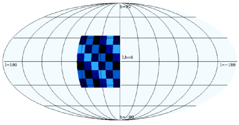
Figure 5: Compact square with 36 zones, covering a 10/used to calculate JK error in galactic coordinates ($l=0^{o}$ to $l=66^{o}$ and $b=-33^{o}$ to $b=33^{o}$). We see that the shapes and sizes of the zones are similar.

2.3 Errors in harmonic space (TH)

Theoretical expectations for the errors are the simplest in Harmonic space where the covariance matrix is diagonal in the all-sky limit. In particular, for Gaussian fields, one can easily see that the variance (or diagonal error) is,

$$\Delta^{2}C^{TG}_{\ell}=\frac{1}{f_{sky}(2\ell+1)}\left[({C^{TG}_{\ell}})^{2}+C^{TT}_{\ell}C^{GG}_{\ell}\right].$$ (14)

This indicates that the variance of the power spectrum estimator results from quadratic combinations of the auto and cross power, with an amplitude that depends on the number of independent $m$-modes available to estimate the power at a scale ${\ell}$, which is approximately given by $f_{sky}(2\ell+1)$. We shall emphasize that this is only approximate and rigorously it is only expected to yield accurate predictions for azimuthal sky cuts. However, as we shall see later, this result is of more general applicability. We note that the dominant contribution to the error and covariance comes from the auto-power of the fields $C^{TT}_{\ell}C^{GG}_{\ell}$ involved in the cross-correlation, whereas the cross-correlation signal $(C^{TG}_{\ell})^{2}$ only gives a few percent contribution, depending on cosmology and survey selection function.

Partial sky coverage introduces a boundary which results in the coupling (or correlation) of different ${\ell}$ modes: the spherical harmonic basis in no longer orthonormal on an imcomplete sky. Thus the covariance matrix between different modes,

$$Cov(C_{\ell},C_{\ell^{\prime}})=<(C_{\ell}-<C_{\ell}>)(C_{\ell^{\prime}}-<C_{\ell^{\prime}}>)>$$ (15)

is no longer diagonal (ie see Fig.7). Because of the partial sky coverage there is less power on the smaller multipoles. This results in a systematic bias on the low multipoles of $C_{\ell}$ that can sometimes be modeled with the appropriate window correction of the survey mask.

Using the Legendre transform one can propagate the error $\Delta C_{\ell}$ in Eq.14 above to configuration space,

$$\Delta^{2}w(\theta)=\sum_{l}\left(\frac{2\ell+1}{4\pi}\right)^{2}~{}P_{\ell}^{2}(\mu)~{}\Delta^{2}C_{\ell},$$ (16)

where $\mu\equiv cos{\theta}$. For the covariance matrix, we find:

$$C_{ij} \equiv Cov(w(\theta_{i}),w(\theta_{j}))$$

$$= \sum_{l}\left(\frac{2\ell+1}{4\pi}\right)^{2}~{}P_{\ell}(\mu_{i})~{}P_{\ell}(\mu_{j})~{}\Delta^{2}C_{\ell},$$

where $\mu_{i}\equiv cos{\theta_{i}}$. Eq(2.3) and Eq(16) assumes that different ${\ell}$ multipoles are uncorrelated which is only strictly true for all-sky surveys. We shall see below that this approximation is quite accurate anyway even for surveys that cover only $10\%$ of the sky, i.e, cosmological parameter contours derived from this expression do not significantly differ from those computed with simulations that take into account the exact covariance matrix.

2.4 Errors in configuration space (TC)

The cross-correlation function in configuration space is estimated by averaging over all pairs of points separated an angle $\theta$ in the survey,

$$w_{TG}(\theta)=<\Delta T(q)\delta_{g}(q^{\prime})~{}\arrowvert_{\hat{qq^{\prime}}=\theta}>_{survey}.$$ (18)

We have derived a formula for the covariance of the estimator in an ensemble of sky realizations. Details of this derivation can be found in Appendix A,

$$C_{ij}={1\over 8\pi^{2}P(\theta_{i})P(\theta_{j})}\int_{0}^{\pi}\frac{K[\theta_{i},\theta_{j},\psi]}{P(\psi)}\sin\psi d\psi$$ (19)

where the kernel $K$ is given by:

$$K[\theta,\theta^{\prime},\psi]={1\over 2}\left[W_{TT}(\theta,\psi)W_{GG}(\theta^{\prime},\psi)+\right.$$ (20)

$$\left.W_{TT}(\theta^{\prime},\psi)W_{GG}(\theta,\psi)\right]+W_{TG}(\theta,\psi)W_{TG}(\theta^{\prime},\psi)$$

and $W_{X}$ is a mean over the corresponding correlation $w_{X}$, with $X=TT,GG$ or $TG$:

$$W_{X}(\theta,\psi)=2\int_{0}^{\pi}d\varphi P(\psi,\theta,\phi)~{}w_{X}(\phi)$$ (21)

where $cos\phi=cos\theta~{}cos\psi+sin\theta~{}sin\psi~{}cos\varphi$. Survey geometry is encoded in $P(\theta)$ and $P(\psi,\theta,\phi)$ probabilities. These are the probabilities for two points separated by an angle $\theta$ or for a triangle of sides $\psi$, $\theta$,$\phi$ to fall completely into the survey area if they are thrown randomly on the full sky. For partial sky surveys these probabilities depend mainly on the survey area and can be well approximated by the formula provided in Appendix A. Particularly simple analytic expressions can be obtained for a “polar cap” survey (area obtained by intersecting a cone with the sphere) and are given in the Appendix B.

This new method of computing errors in real space has several advantages. Since it takes into account the survey geometry, it can provide more accurate errors at large angles where both the jackknife errors and the harmonic-space errors become more inaccurate. Compared to montecarlo errors this method is faster because one does not need to generate a large number of sky realizations. What is more, this estimator does not need to rely on any theoretical/fiducial model and one can readily apply it to correlation functions measured on the real data to estimate the errors.

Figure 6: Normalized covariances in real space for different methods as labeled in the figure. No significant changes are found for different methods and sky fractions used.

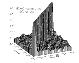
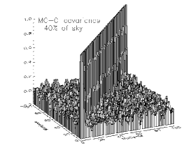
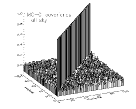
Figure 7: Normalized covariances in $C_{\ell}$ space from montecarlo (MC2) method. The covariance becomes progressively dominated by its diagonal elements as we increase the sky fraction $f_{sky}$.

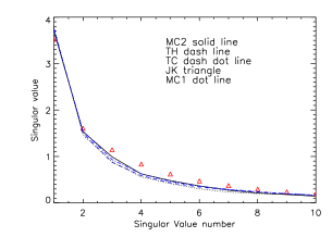
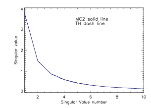
Figure 8: Eigenvalues in real space for 10% sky (left panel) and all sky (right).

Figure 9: Eigenvectors in real space for 10% of the sky and for all sky, as labeled in each panel. First eigenvector is shown as solid lines, second as dotted, third dashed and fourth dot-dash. Results for $MC1-w$ and $TC-w$, not shown here, are very similar.

3 Normalized Covariance Matrix

For each one of the methods presented in the previous section, we next compare the normalized covariance:

$$\widehat{C}_{ij}=\frac{C_{ij}}{\sqrt{(C_{ii}C_{jj})}}$$ (22)

The diagonal values (the variance) and associated dispersion will be investigated in §4.

3.1 Configuration space

As shown in Fig.6 all the normalized covariances $\widehat{C}_{ij}$ in real space are very similar. The appearance of the plots does not seem to depend strongly on the method we use to estimate them, or the survey area $f_{sky}$. Here we only show results for 10% and all the sky, but intermediate values yield similar results. However, we want to question if slight differences in the covariance could have a non-negligible impact on cosmological paramter estimation. We will discuss this in detail in §5.3.

3.2 Harmonic space

In $C_{\ell}$ space, there is no correlation between different $l$-modes (bins $\Delta{\ell}=1$) for the case of all sky (MC2) maps. The normalized covariance matrix is diagonal, as can be seen in the right panel of Fig.7. Also shown, in the left and central panels, are the results for 10% and 40% of the sky, where the covariance between modes gives rise to large amplitude off-diagonal elements. This is in sharp contrast to the results in configuration space (in Fig.6) where there is no significant difference between normalized covariances in real space when we decrease the area. This is because the main effect of increasing the area in configuration space is the reduction of diagonal errors (which are shown in next section), while in harmonic space there is a transfer of power from diagonal to off-diagonal elements.

3.3 Eigenvalues and Eigenvectors from SVD

To calculate the distribution $\chi^{2}$ and the signal to noise we need to invert the covariance matrix. We use the Singular Value Decomposition method to decompose the covariance in two orthogonal matrices $U$ and $V$ and a diagonal matrix $W$ which contains the singular values $\lambda_{i}$ squared on the diagonal (eg see Press etal 1992). This method is adequate to separate the signal from the noise:

$$\widehat{C}_{ij}=(U_{ik}^{T})W_{kl}V_{lj}$$ (23)

where $W_{ij}=\lambda_{i}^{2}\delta_{ij}$ and $\widehat{C}_{ij}$ is the normalized covariance in Eq.22. By doing this decomposition, we can choose the number of modes that we wish to include in the analysis. This SVD is effectively a decomposition in different modes ordered in decreasing amplitude.

We obtain very similar singular values for each mode and for each method, as show in Fig.8 for some of the cases (other cases give very similar results).

We can understand the effect of modal decomposition looking at the eigenvectors shown in Fig.9, where we have plotted the four dominant eigenvectors as a function of angle: first mode (solid) affects only the amplitude, second mode (dotted) shows a bimodal pattern. The following modes, third (dashed) and fourth (dot-dash), correspond to modulations on smaller angular scales. As can be seen in the Figure, we obtain nearly the same eigenvectors in all the cases, in agreement to what was found by direct comparison of the covariance matrices in Fig.6. Again, we can ask: are the small differences significant? We will study this in detail in §5.

4 Variance & errors

4.1 Variance in $w(\theta)$

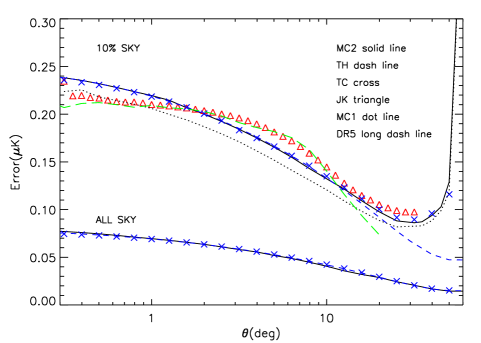
Figure 10: Error calculated with different methods (as labeled in the figure) in real space for $\Omega_{DE}=0.7$. For a map covering $10\%$ of the sky (top lines and symbols), the TC (crosses) and TH (dashed line) theoretical errors work well compared to the montecarlo MC2 simulations (solid line), while MC1 simulations (dotted line) seems to underestimate the errors by 10%. The JK method (triangles) seems slightly biased up/down on large/small scales, although all the errors are compatible given the sampling variance dispersion we expect (see Fig. 12). For all sky maps (bottom lines and symbols), we show how results for MC2 (solid), TH (dashed) and TC-w (cross) agree very well.

Fig.10 is one of the main result of this paper. We compare the variance for the different methods, which is the diagonal part of the covariance matrix. By construction, in the limit of infinite number of realizations, the MC2 error from simulations should provide the best approximation to the errors. We have demonstrated (in section §2.1.2) that 1000 simulations are enough for convergence within $5\%$ accuracy. For all sky maps (lower lines in the Figure) we can see that the three methods used: MC2-w, TH-w and TC-w, yield identical results, as expected. For smaller survey areas we do expect some deviations, because of the different approximations on dealing with the survey boundary. For a survey covering 10% of the sky these 3 methods also agree well up to 10 degrees. At larger scales TH-w (dashed lines) starts to deviate, because boundary effects are in fact not taken into account in this method. The JK error (triangles) has a slope as a function of $\theta$ that seems less steep than the other methods, but still gives a reasonably good approximation given that the dispersion in the errors is about $20\%$ (as discuss in §4.3 below). Note how on scales larger than 10 degrees the JK method performs better (ie it is closer to MC2) than the TH-w error. The TC method seems to account well for the boundary effects, as it reproduces the MC2 errors all the way to 50 degrees, where all other methods fail.

If we only use one single realization for the galaxies (MC1) the error seems to be systematically underestimated by about $10\%$ on all scales. This bias is expected as we have neglected the variance in the galaxy field and the cross-correlation signal. A particular case of MC1 is done with real data from SDSS DR5 (shown as long dashed line in Fig.10). We have used here a compact square of 10% of the sky from the SDSS $r$ magnitude slice of 20-21, which has a redshift selection function similar to the one in our simulations ($z_{m}=0.33$). This case works surprisingly well once scaled with linear bias $b$ (estimated by comparing the measured galaxy auto-correlation function with the one in our fiducial $\Lambda$CDM model). It happens to closely follow the JK prediction, rather than the MC1 prediction, but we believe this is just a fluke, given the dispersion in the errors (see §4.3) and the uncertainties in the fiducial model.

4.2 Effect of partial sky coverage

Figure 11: Error at a two fix angles: 5 deg (upper lines) and 20 deg (lower lines) as a function of $f_{sky}$, the fraction of the sky covered by the map. As predicted, errors decrease as $1/\sqrt{f_{sky}}$ in both cases. Note how for small areas, the TC-w prediction (continuous line) performs better than the TH-w model (dashed line) as it better reproduces the MC2 simulations (squares).

We have tested MC2-w, TH-w and TC-w for different partial sky survey areas $f_{sky}$ and obtained similar results. In Fig.11 we have plotted the error for a fix angle of 5 degrees (top) and 20 degrees (bottom) for the different values of $f_{sky}$. The three methods coincide for large areas. The error scales by a factor $1/\sqrt{f_{sky}}$, as expected.

Notice that errors at angles comparable to the width of the survey are difficult to estimate theoretically because one needs to take into account the survey geometry. Even for a map as wide as $10\%$ of the sky, the survey geometry starts to be important for errors in the cross-correlation above 10 degrees. This is shown in simulations as a sharp inflection that begins at 30 degrees in Fig. 10 (solid line) . Our new TC-w method predicts well this inflection, while the more traditional TH method totally misses this feature. This can also be seen in Fig.11 for 20 degrees when we approach small values of $f_{sky}$.

4.3 Uncertainty in $w(\theta)$ errors

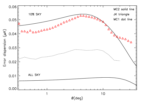
Figure 12: Dispersion of the error calculated with different methods in real space for $\Omega_{DE}=0.7$. For MC2-w (solid line) or MC1-w (dotted lines), we take each pair of MC2 or MC1 simulations as the input for the error in the TH-w calculation in Eq.16 . For JK (triangles), we have one error for each MC2 simulation. We can see how the error in the error is of other $~{}20\%$ for MC2 or JK and is lower for MC1 (mainly because one of the maps in each pair is kept fixed). The lower line corresponds to the dispersion in all sky maps.

To assess the significance of the differences in the error estimation that we find using different methods, we will compute here the sampling uncertainties associated with error estimation. Fig.12 shows the sampling dispersion in the error estimates. This can be calculated from the TH and TC approaches by using $C_{\ell}$ or $w(\theta)$ measure in each realization as the input model for theoretical predictions (Eq.16 or Eq.19). In Fig.12 solid (or dotted) line shows the result of using Eq.16 for each of the MC2 (or MC1) simulations. This produces an error for each realization and we can therefore study the error distribution. The uncertainty in the error (or error in the error) correspond to the rms dispersion of this distribution. We need all the multipoles to compute this Legendre transformation (Eq.16) although we lose some information for low multipoles when we use only a fraction of the sky. The error propagation Eq.16 is not linear and we find that this produces a bias of $3\%$ when we compare the mean of the propagated errors in each simulation with the propagation of the mean error in all simulations.

We can also calculate the JK-w dispersion of the error, because we have the JK error for each MC2 simulation (remember that we only need one realization to obtain the JK error). The JK-w dispersion (triangles) in Fig.12 is quite close to the MC2-w values. They are both of the order of $20\%$ relative to the mean error. This uncertainty can be interepreted as the result of the uncertainties in our input model; typically the model is only known to the accuracy given by the data and a given sky realization will deviate from the ’true’ model (i.e, the mean over realizations). Thus, if one chooses to use the estimated values from the data (or it’s bets fit model) as input to the error estimation, this produces an uncertainty in the error which is of the order of this scatter. This is always the case with the JK errors, which do not use any model, but the uncertainty is similar if we use direct measurements as input to the other error estimations, as shown in Fig.12.

For completeness, Fig.12 also shows the dispersion for the MC1 error (dotted). There is less dispersion in the MC1 method because one of the maps is always fixed and this reduces both the error and, more strongly, its dispersion.

4.4 Error distribution for JK

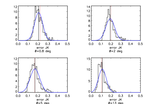
Figure 13: Histograms show the error distribution in JK errors from 1000 simulations at different angles. Solid line shows a Gaussian with the same mean and dispersion. Vertical lines correspond to mean JK error (solid) and the true mean MC2 error (dotted).

Fig.13 shows the distribution of JK errors in the MC2 simulations as compared to a Gaussian fit with the same mean and dispersion. Each panel shows the distribution of $w(\theta)$ errors at a given fixed angle. The mean MC2-w error (shown as solid line in Fig.10) is shown here by a dotted vertical line, while the mean of the JK errors (shown as triangles in Fig.10) corresponds here to the continuous vertical line. We can see here how the MC2-w error and the mean JK-w error are quite similar. The variance in the distribution agrees with the results in §4.3 above. Note also that the JK distribution of $w(\theta)$ errors can be well fitted by a Gaussian. This is important for two reasons. First it shows that there are no important outliers or systematic bias when one uses a JK estimator in a single realization, as is the case with real data. Second, it indicates that the error in the error (ie the rms dispersion of this distribution) entails all relevant information needed to asses in more detail the accuracy of the JK error analysis. One could for example fold the uncertainties in this distribution to asses the significant of a detection.

4.5 Variance in $C_{\ell}$

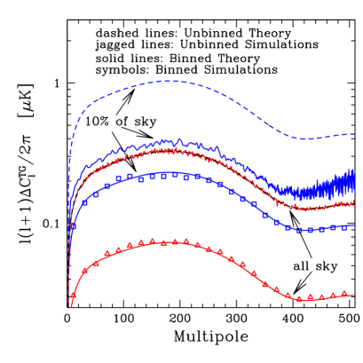
Figure 14: Errors in $C_{\ell}$ space calculated with (MC2) simulations as compare to (TH-$C_{\ell}$) theory. For all sky maps, the theoretical prediction works well, but for 10% of the sky we see a big discrepancy between theory (dashed lines) and simuations (jagged lines). This is due to covariance between modes and can be solved by binning the $C_{\ell}$ spectrum, as shown by the symbols (simulations) and sold line (predictions in Eq.24).

In $C_{\ell}$ space, we have compared MC2 errors to TH theory. Fig.14 shows how both errors are hard to distinguish for the case of all sky (middle dashed line matches closely the jagged line). Note the shape of the $C_{\ell}$ errors exhibits a broad peak around $\ell=200$ illustrating the fact that errors are dominated by the $C_{\ell}^{T}T$ term. For 10% of the sky the TH error (upper dashed line) obtained theoretically from Eq.14 (with a factor $1/\sqrt{f_{sky}}$ respect to all the sky) is much larger than the MC2 error (upper jagged line) in the simulations. As we have shown in Fig.7, there is a strong covariance between different bins when $f_{sky}<1$, this is in contrast with the TH estimation in Eq.14 which assumes a diagonal covariance matrix. We understand this discrepancy in the variance prediction as a transfer of power from the diagonal to off-diagonal errors.

We can get a better diagonal error estimation by binning $C_{\ell}$ in a $\Delta\ell$ that makes the covariance approximately diagonal. When binning by $\Delta\ell$, the theoretical error (TH-Cl) in Eq.14 is reduced in quadrature to:

$$\Delta^{2}C^{TG}_{\ell}=\frac{1}{\Delta\ell f_{sky}(2\ell+1)}\left[({C^{TG}_{\ell}})^{2}+C^{TT}_{\ell}C^{GG}_{\ell}\right],$$ (24)

This assumes that the bins are independent. Because of the partial sky coverage, the bins are not independent and the above formula will only be valid in the limit of large $\Delta\ell$.

We have tested the above formula for different sky fractions by binning the $C_{\ell}$ spectrum in the simulations and estimating the error from the scatter in different realizations. We find that the formula works above some minimum $\Delta\ell$ which roughly agrees with the width of off-diagonal coupling in the covariance matrix estimated from simulations (Fig.7). We find that $\Delta\ell$=20,16,8,1 for $f_{sky}$=0.1,0.2,0.4,0.8 respectively, diagonalize the covariance matrix and provide a good fit to the above theoretical error for binned spectra. In Fig.14 we show the results for $\Delta\ell=20$ for both all sky (triangles) and 10% of the sky (squares). The theoretical prediction in Eq.24 (solid lines) works very well in both cases, because the covariance with this binning is approximately diagonal.

4.6 Dependence on $\Omega_{DE}$

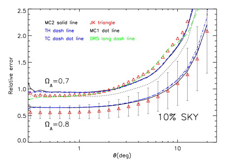
Figure 15: Relative error for the two fiducial models $\Omega_{DE}=0.7$ (top) and $\Omega_{DE}=0.8$ (bottom). The different methods are labeled in the figure. We see that the relative error depends on the model, and that in the case $\Omega_{DE}=0.8$ there is also a good agreement within the errors.

Fig.15 shows a relative comparison of how our error estimation changes for a different cosmology with $\Omega_{DE}=0.8$ instead of $\Omega_{DE}=0.7$. The MC error still fits well the TH and TC predictions, but the JK errors seem to underestimate the errors more than in the $\Omega_{DE}=0.7$ case. This effect is not large given the dispersion in the errors from realization to realization (errorbars in Fig.15).

5 Constraints and significance

ISW measurements can directly constrain dark-energy parameters independent of other cosmological probes. Here we shall use the covariance analysis presented in the previous section to derive significance levels for the cosmological parameter constraints obtained from a cross-correlation analysis.

5.1 Signal-to-noise from $w(\theta)$

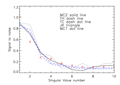
Figure 16: Signal-to-noise for 10% of the sky for each singular value. Different lines correspond to methods as labeled.

$S/N$	10%	20%	40%	80%	all sky
Simulations MC2-w	1.2	1.7	2.5	3.5	3.8
Theory TH-Cl	1.2	1.7	2.4	3.4	3.8
Theory TH-w	1.2	1.7	2.4	3.4	3.8

Table 2: Signal-to-noise as a function of $f_{sky}$ covered in a survey with a broad distribution of sources with median redshift $z_{m}=0.33$ for the $\Omega_{DE}=0.7$ flat $\Lambda$CDM model with different error assumptions (see TableLABEL:notation). Similar results are found for TC-w and JK-w methods.

The signal-to-noise ($S/N$ hereafter) depends on both the input fiducial model used in the simulations and the covariance matrix method we implement. In this paper we shall invert the covariance matrix using the standard method of singular value decomposition (SVD), see §3.3. In this approach one projects the signal to the eigenvector space of the thus diagonalized matrix and only the most significant eigenvalues are kept for the analysis,

$$\Big{(}\frac{S}{N}\Big{)}_{i}=\Big{|}\frac{\widehat{w}_{TG}(i)}{\lambda_{i}}\Big{|}=\Big{|}\frac{1}{\lambda_{i}}\sum_{j=1}^{N_{b}}U_{ji}\,\frac{w_{TG}(j)}{\sigma_{w}(j)}\Big{|}.$$ (25)

Fig.16 shows the S/N for each singular value. All methods agree well even for 10% of the sky. We get excellent agreement for all sky maps.

Because eigenvectors are orthogonal the total S/N is just added in quadrature:

$$\Big{(}\frac{S}{N}\Big{)}_{T}^{2}=\sum_{i}~{}\Big{(}\frac{S}{N}\Big{)}_{i}^{2}$$ (26)

Table 2 compares total S/N values from simulations and theory for different survey areas. Here by Simulations we mean the MC2-w method where we have used 6 singular values and theory refers to the different methods, including the TH-$C_{\ell}$ approach (see below). We note that we find apparently lower values than quoted in the literature (see e.g, Afshordi 2004). This is due to the low value adopted for $\Omega_{DE}$ (i.e $\Omega_{DE}=0.8$ models yield a S/N ratio $\sim 2$ larger than our fiducial value $\Omega_{DE}=0.7$), and the fact that these are predictions for a single broad redshift bin (similar to the selection function for SDSS main sample galaxies), with median redshift $z_{m}=0.33$. A combination of several narrow bins at different redshifts will also increase the S/N (see Fig.17 and Table 3 below).

5.2 Signal-to-noise forecast from $C_{\ell}$

In harmonic space the $S/N$ is estimated as

$$\Big{(}\frac{S}{N}\Big{)}_{T}^{2}=\sum_{\ell}\Big{(}\frac{C^{TG}_{\ell}}{\Delta C^{TG}_{\ell}}\Big{)}^{2}$$ (27)

using Eq. 14 in the denominator. Note in particular that the dominant contribution to $\Delta C_{TG}$ in Eq. 14, comes from the $C_{TT}~{}C_{GG}$ term and not from $C_{TG}$ which is an order of magnitude smaller. This means that the $(S/N)^{2}$ approximately scales as:

$$\Big{(}\frac{S}{N}\Big{)}_{T}^{2}\simeq\sum_{l}\frac{C^{TG}_{\ell}~{}C^{TG}_{\ell}}{C^{GG}_{\ell}~{}C^{TT}_{\ell}}\propto\sigma_{8}^{2}$$ (28)

and therefore depends strongly on the normalization of the dark matter power spectrum $P(k)$, and is independent of the galaxias bias $b$.

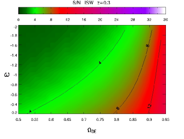
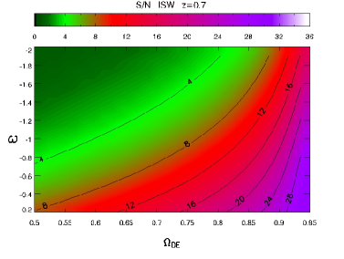
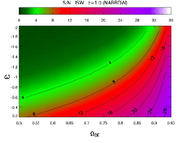
Figure 17: All sky values of the S/N for different models. Each panel corresponds to different redshift distribution: SDSS ($z_{m}=0.3$), DES($z_{m}=0.7$), DES+VISTA ($z_{m}=1$) and DES+VISTA NARROW ($z_{m}=1$). Expectations for smaller survey areas are obtained by scaling the displayed values by $\sqrt{f_{sky}}$, where $f_{sky}$ is the sky fraction covered.

$S/N$	$z_{m}=0.33$	$z_{m}=0.7$	$z_{m}=1$	$z_{m}=1$ (N)
$\Omega_{DE}=0.7$	3.8	6.0	6.3	4.2
$\Omega_{DE}=0.8$	5.5	9.5	10.6	7.6

Table 3: Signal-to-noise for all sky maps in harmonic space for two different values of $\Omega_{DE}$ and for galaxy maps with different mean depths $z_{m}$. The width of the redshift distribution is given by $\sigma_{z}\simeq z_{m}/2$ (see Eq.3) except in the last case ($z_{m}=1$ Narrow), where $\sigma_{z}\simeq 0.17$

Clearly, the S/N will change depending on the fiducial model used. Fig. 17 shows this dependence on the plane DE density vs. equation of state, $w$. Each panel corresponds to different smooth redshift distributions that closely match current or planned surveys. The upper panels show predictions for SDSS main sample ($z_{m}=0.33$), that anticipated for the DES ($z_{m}=0.7$), and a combined DES+VISTA survey ($z_{m}=1$), respectively. For these 3 surveys we use broad distributions as given by Eq.(3), with a width that grows linearly with depth, $\sigma_{z}\simeq z_{m}/2$. For this rather generic parametrization of the selection function, the S/N monotonically increases with $z_{m}$ as shown by the 3 upper panels in Fig.(17), although the differential contribution, $d(S/N)/dz$, drops for sources at $z\lower 2.15277pt\hbox{$\;\buildrel>\over{\sim}\;$}0.4$ (see Afshordi 2004 for an analytic account of this effect).

In particular, for our baseline survey, SDSS, and our fiducial $\Lambda$CDM model, we estimate $S/N=3.8$, what is in good agreement with simulations in configuration space (see Table 2). As we sample a wider range of the ISW signal in redshift, the S/N raises by $\sim 60\%$ when we increase the survey depth by a factor $\sim 2$ to match the depth of the DES-like survey. However, there is little gain in ISW detection significance when combining DES+VISTA, as the S/N only increases by an additional $5\%$ with respect to the DES survey. For comparison, we also show the case of what we shall call DES+VISTA NARROW survey. This survey has a Gaussian distribution of sources around $z_{m}=1$, but with a narrow width, similar to that of SDSS above ($\sigma_{z}=0.17$). In this case, the high redshift population of sources brings a poor added value to the baseline survey (SDSS) by improving the S/N by only $10\%$. As shown in Table 3 these conclusions vary somewhat for different values of $\Omega_{DE}$.

We point out that in these estimations we have ignored the lensing magnification bias contribution (see Loverde, Hui & Gaztañaga 2006) which could be important for $z>1$.

5.3 $\chi^{2}$ estimation

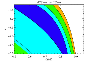
Figure 18: $\chi^{2}$ contours from (MC2-w) simulations (in color) compared to the other methods (solid line): JK-w, MC1-w, TC-w, TH-w, TH-$C_{\ell}$ as labeled in each panel. All cases correspond to 10% of the sky. The contour levels are: 0.25, 1., 4. and 9.

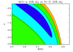
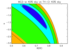
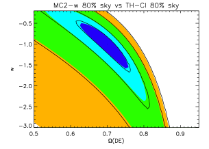
Figure 19: Same as Fig.18, but here each panel compares to the method TH-$C_{\ell}$ for 20%, 40% and 80% of the sky.

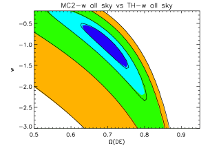
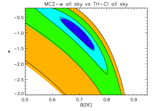
Figure 20: Same as Fig.18 for all sky maps. Here solid lines correspond to methods TH-w (left panel) and TH-Cl (right panel).

We shall discuss below to what extent the choice of covariance matrix estimation method affects cosmological parameter constraints. This is specially relevant because current ISW detection significance levels are still rather poor (i.e, at the 4-$\sigma$ level at most, see Cabre etal 2006) and the practical implementation of methods might yield noticeably different results.

We shall compare the methods described in §3, whereas the fiducial model is the one implemented in the simulations. Our significance levels are derived from a $\chi^{2}$ statistic:

$$\chi^{2}=\sum_{i,j=1}^{N}\Delta_{i}~{}\hat{C}_{ij}^{-1}~{}\Delta_{j}$$ (29)

where:

$$\Delta_{i}\equiv\frac{(w_{TG}^{E}(\theta_{i})-w_{TG}^{M}(\theta_{i}))}{\sigma_{TG}(\theta_{i})}$$ (30)

is the difference between the ”estimation” $E$ and the model $M$. We have run models for $\Omega_{DE}$ from 0.5 to 0.9 and for $w$ from -3.0 to -0.2 and we fix the estimation $E$ to be our fiducial model $\Omega_{DE}=0.7$ and $w=-1$ which was input in the simulation. The size of the resulting confidence level contours depends implicitly on the best-fit model (i.e, the fiducial model) by construction.

In each case, the error used is the one obtained from the simulations (for cases MC2-w, MC1-w, JK-w, MC2-$C_{\ell}$) or from the theoretical estimator (TH-w and TH-$C_{\ell}$) for the given fiducial model. That is, the errors are not varied as we sample parameter space in the $\chi^{2}$ estimation. This allows a direct comparison on the contours when using different covariance matrix estimators.

Results are shown in Fig.18,19 and 20. In the different figures we compare the real space MC (MC2-w) result (colored contours) with the other methods (contours traced by solid lines). Contours from different methods agree remarkably well: it does not depend neither on which space we compute the errors and covariance (real or harmonic space), nor in the portion of the sky used. We have checked that small contour differences are compatible once we take into account uncertainties in the errors, as shown in Fig.12. Moreover using a diagonal approximation for the $C_{\ell}$ covariance matrix to infer the covariance in real space (through the Legendre transform in Eq.16), works for a small portion of the sky surprisingly well. As explained in section $\S$4.5, when we use the theoretical error in $C_{\ell}$ space (TH-$C_{\ell}$) for real data, we should use a bin of width of $\Delta l$ that varies with the portion of the sky.

5.4 Best fit model

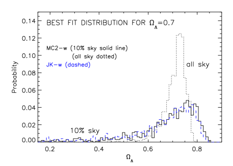
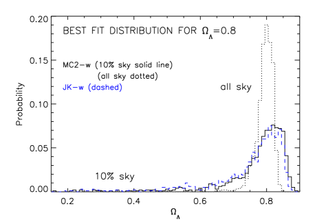
Figure 21: Distribution of best fit values for $\Omega_{DE}$ fixing $w=-1$ and all the other parameters to the fiducial model. For JK (dotted lines), we use the JK-w error obtained for each simulation. For the MC2 simulations (solid line), we use a fixed error obtained from the dispersion in the simulations.

In this section we investigate how the error method used affects the best fit estimation of cosmological parameters. We fix all the parameters as in the fiducial model, except for $\Omega_{DE}$. We focus on the case of the angular 2-point correlation $w(\theta)$ and compare results for JK-w to those for MC2-w. We do a $\chi^{2}$ fit of the correlation from each single simulation, which is used as the ”E” estimator in Eq.30. This follows what is done with real data where the observations correspond to a single realization. We can make a distribution for all the best fit values of $\Omega_{DE}$ that we obtain from each realization, which is shown in Fig.21. The error and covariance used in the fit is in one case the JK-w obtained using this single simulation (dashed line in Fig.21) or the MC2-w calculated from all the simulations (continuous line). Despite these differences there is an excellent agreement between the JK-w and the MC2-w results.

We see that the distribution of best fit values is biased towards higher values than the underlying fiducial model value $\Omega_{DE}=0.7$. In partiuclar, the distribution of best-fit values is skewed, showing a long tail of values smaller than the input model. This is due to the fact that contours in $\chi^{2}$ (and in the S/N) are not symmetric. The reason for this is the nonlinear mapping between values of $\Omega_{DE}$ and the amplitude of $w(\theta)$. When the errors are large, this non-linear mapping transforms an approximate Gaussian distribution (which is a good approximation for the distribution of $w(\theta)$) into a strongly non-Gaussian distribution in $\Omega_{DE}$. When the errors are smaller, as happens for larger $\Omega_{DE}$, the mapping between $w(\theta)$ and $\Omega_{DE}$, is better approximated by a linear relation which results in a more Gaussian distribution. Thus, if we have small enough errors, this bias is negligible, as we can see for the all-sky case shown by the dotted lines in Fig.21.

6 Summary & Conclusions

We have run a large number of pairs of sky map simulations, that we call MC2. Each pair is a stochastic realization of an auto and cross correlation signal, that we input to the simulation, what we call the fiducial model. We have focused our attention in testing the galaxy-temperature cross-correlation, so each pair of simulations correspond to a CMB and a galaxy map. For the fiducial model we take the current concordance $\Lambda$CDM scenario. We have run simulations for different values of $\Omega_{DE}$ and have tested maps with different fractions of the sky. We have concentrated on the case $\Omega_{DE}=0.7$ and $f_{sky}=0.1$ which broadly matches current observations and results in large errors ($>50\%$).

We are interested in error analysis/forecast and significance estimation. We calculate the correlation between maps and use the different realizations to work out the statistics. We then compare the results to the different approximations that have been used so far in the literature. One of the approximations, that we call MC1, uses montecarlo simulations for the CMB maps with a fixed (observed) galaxy map (ie with no cross-correlation signal or sampling variance in the galaxies). We test a popular harmonic space prediction, that we shall call TH (Theory in Harmonic space). We also test Jack-Knife (JK) errors which uses sub-regions of the actual data to calculate the dispersion in our estimator. Finally, we introduce a novel error estimator in real space, that call TC (Theory in Configuration space). For both models and simulations we have assumed that the underlaying statistics in the maps is Gaussian. Our main results can be summarized as follows:

1. The number of simulations needed for numerical convergence (to within $\simeq 5\%$ accuracy) in the computation of the covariance matrix is about 1000 simulations (see §2.1.2).

2. Diagonal errors in $w(\theta)$ are very accurate in both TH and TC approximations for all sky maps. This is shown in the bottom lines of Fig.10. For maps with different fraction of the sky $f_{sky}<1$, the agreement is also good on small scales ($\theta<20$ deg) as can be seen in Fig.11.

3. Even for a map as wide as $10\%$ of the sky, the survey geometry starts to be important for errors in the cross-correlation above 10 degrees. This is shown in simulations as a sharp inflection that begins at 30 degrees in Fig. 10 (solid line) . Our new TC method predicts well this inflection, while the more traditional TH method totally misses this feature.

4. If we only use one single realization for the galaxies (MC1) the error seems to be systematically underestimated by about $10\%$ on all scales. This bias is expected as we have neglected the variance in the galaxy field and the cross-correlation signal.

5. The JK errors do quite well within 10% accuracy on all scales, including the larger scales where boundary effects start to be important (see triangles in Fig.10).

6. The dispersion in the error estimator (error in the error) for individual realizations is of the order $~{}20\%$ (see Fig.12). This uncertainty is inherent to the JK method, because one uses the observations (a single realization) to estimate errors. But it is also implicit in other methods because our knowledge of the models is limited by the data and can be thought of as a “sampling variance error”.

7. S/N (see Fig.16) and parameter estimation (see Fig. 20 and Table 2) are equivalent when we do the analysis in configuration and harmonic space. This was expected for all sky maps, but it is not trivial for partial sky coverage (see comments below).

8. It is possible to propagate errors and covariances from $C_{\ell}$ to $w(\theta)$ (harmonic to configuration space) using Eq.(16). Starting from a diagonal (all sky) covariance matrix in $C_{\ell}$, the resulting covariance matrix in $w(\theta)$ is quite accurate as compared to direct estimation from simulations.

9. The above propagation also works well for a map with a fraction $f_{sky}$ of the sky, by just scaling the $C_{\ell}$ errors by a factor $1/\sqrt{f_{sky}}$ respect to all the sky. This is surprising because for $f_{sky}<1$ the covariance matrix in $C_{\ell}$ is no longer diagonal (see Fig.7) and the actual measured $C_{\ell}$ errors in simulations do not simply scale with $1/\sqrt{f_{sky}}$ (see Fig.14). Thus, Eq.(16) should not be valid. We believe that this works because the two effects compensate. There is a transfer of power from diagonal to off-diagonal elements of the covariance matrix which for the scales of interest (smaller than the survey area) seems to corresponds to a rotation that somehow does not affect the final errors from Eq.(16).

10. If we want to use the popular TH approach in Eq.(14) with $f_{sky}<1$ we need to bin the $C_{\ell}$ data in multipole bands of width $\Delta\ell$. The binned spectrum has a diagonal covariance when $\Delta l$ is large enough and the error in the binned spectrum approximately follows Eq.(24).

11. When the errors are large (i.e., for partial sky coverage and $\Lambda$CDM models with not so large $\Omega_{DE}$) there is a signficant bias in the distribution of the recovered best-fit values of $\Omega_{DE}$, as shown in Fig.21. This is because of the non linear mapping between $\Omega_{DE}$ and the amplitude of $w(\theta)$.

12. S/N forecasts for future surveys, shown in Fig.17 and Table 3, strongly depend on the fiducial model used. For example, an all-sky survey with broadly distributed sources around a median redshift $z_{m}=1$ and $\Omega_{DE}=0.8$ can detect the ISW effect with a S/N$\simeq 11$.

What method should be used when confronted with real data? Running realistic simulations seems the best approach, but is very costly because we need of order 1000 simulations for each model we want to explore. The theoretical modeling of errors seems quite accurate and is much faster to implement. The main advantage of the JK approach is that the errors are obtained from the same data in a model independent way. This is important because real data could surprise our prejudices and also because, in the ISW case, the errors are very large and the data can accommodate different models.

As an example, consider the analysis of Cabre etal (2006) who recently cross-correlated the SDSS-DR4 galaxy with the WMAP3 CMB anisotropies. Using the JK approach with $w(\theta)$ they estimate a $S/N\simeq 3.6$ for the $r=20-21$ sample, which has a mean redshift of $z_{m}\simeq 0.33$. These numbers are high compared with the values in Table 3 for $z_{m}=0.33$ which for $f_{sky}=0.13$ gives a low $S/N\simeq 2$, even for $\Omega_{DE}=0.8$. The dominant contribution to the S/N in Table 3 scales as $C_{\ell}^{TG}/\sqrt{C_{\ell}^{GG}}$ (ie see Eq.28) and is therefore independent of bias, but depends on $\sigma_{8}$. We have noticed that in fact the actual measured values of $C_{\ell}^{TG}/\sqrt{C_{\ell}^{GG}}$ in the SDSS DR4-WMAP3 maps are almost a factor of 2 larger than the values in the concordance $\Omega_{DE}=0.8$ ($\sigma_{8}=0.9$, $n=1$, $\Omega_{\nu}=0$, $\Omega_{B}=0.05$, $h=0.7$) model. This explains the discrepancy in the $S/N$ and illustrates the danger of blindly using theoretical errors that are model dependent. The discrepancy of the concordance model with the SDSS4-WMAP3 measured values of $C_{\ell}^{TG}/\sqrt{C_{\ell}^{GG}}$ is not very significant once we account for sampling errors (less than 3-sigma), but it could be an indication of new physics that make the $P(k)$ normalization higher than the concordance model, ie deviations in $\sigma_{8}$, spectral index $n$, neutrinos $\Omega_{\nu}$, etc, away from the fiducial model we are considering.

We have also shown that it is possible to use the other theoretical models (ie TC and TH) to make model independent error predictions from observations. Contrary to all other methods, the JK approach does not assume Gaussian statistics, but its accuracy could depend on the model or the way it is implemented (ie shape and number of sub-regions). We conclude that to be safe one needs to validate the JK method with simulations, but there is no reason apriori to expect that this method is inaccurate.

In summary, we have presented a detailed testing of different error approximations that have been used in the literature, both in configuration and harmonic space. Contrary to some claims in the literature (see Introduction), we show that the different errors (including the JK method) are equivalent within the sampling uncertainties. By this we mean not only that the error and covariance are similar but also that they produce very similar signal-to-noise (S/N) and recovery of cosmological parameters.

Appendix A Covariance matrix and errors in configuration space

A.1 The estimator

Consider two fields in the sky $A(q)$, $B(q^{\prime})$ which correpond to one realization of the universe. We want to estimate the true two point cross-correlation function of the universe $w_{AB}$ by averaging over the sky in the survey area $S$. The estimator is

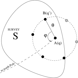
Figure 22: Representation of the $\widehat{w}_{AB}(\theta)$ estimator. The product AB is averaged in an ordered way over all pairs of $\theta$-separated points that belong to the survey area (black points).

$$\widehat{w}_{AB}(\theta)=<A(q)B(q^{\prime})\arrowvert_{\hat{qq^{\prime}}=\theta}>_{S}$$ (31)

where we average over all pairs separeted by an angle $\theta$ and $\theta+\Delta\theta$ in the survey region. This can be put in an integral form

$$\widehat{w}_{AB}(\theta)={1\over S_{N}}\int_{S}dqdq^{\prime}\arrowvert_{\hat{qq^{\prime}}=\theta}A(q)B(q^{\prime})={1\over 4\pi 2\pi\sin{\theta}\Delta\theta P(\theta)}\int_{S}dq\int_{0}^{2\pi}\sin{\theta}\Delta\theta d\varphi A(q)B(q+\theta(\varphi))D(q,\theta,\varphi)$$ (32)

where $S_{N}$ is the normalization factor and the integral is over $dq\in S$ and $d\varphi\in(0,2\pi)$. As it is illustrated in Fig (22), we integrate all the pairs in an ordered way. First, we fix a point $q$ and sum over all the $\theta$-separated pairs related to this point, moving around $\varphi$. Since not all the points in the sky $\theta$-separated from $q$ belong to the survey, we introduce a selection function $D(q,\theta,\varphi)$ which is one if the second point belong to the survey and zero otherwise. We perform this operation in each point of the survey. The origin of $\varphi$ is not relevant, it could be taken for instance as the direct angle between the $\theta$-pair and the geodesic line between the $q$ point and the pole. The second integration is over all the points in the survey.

The normalization factor $S_{N}$ is a measure of the number of $\theta$-pairs allowed by the survey, which depends on $\theta$. For an all sky survey, $S_{N}$ is $4\pi 2\pi\sin{\theta}\Delta\theta$. The geometry of the survey is enclosed in a multiplicative factor $P(\theta)$, which is actually the ratio between the number of $\theta$-pairs in the survey and the number of $\theta$-pairs in the whole sky, i.e., the probability that when throwing a $\theta$-pair in the whole sky it falls into the survey. When $\theta=0$, this probability is equal to the fraction of sky $f_{sky}$ covered by the survey. In an all sky survey, $P(\theta)=1$ and also $D(q,\theta,\varphi)=1$, and the estimator for the cross-correlation is given by:

$$\widehat{w}_{AB}(\theta)={1\over 4\pi 2\pi}\int dqd\varphi A(q)B(q+\theta(\varphi))$$ (33)

A.2 Covariance

In order to get the covariance, we need to relate the estimator of the cross-correlation with the true cross-correlation value. The true cross-correlation value $w_{AB}(\theta)$ is the average over realizations of the estimator, (where the estimator $\widehat{w}_{AB}(\theta)$ is obtained averaging for all the $\theta$ of the sky). Due to homogeneity, $w_{AB}(\theta)$ is also equal to average any $\theta$-pair of fixed points A and B over all the realizations.

$$w_{AB}(\theta)=<\widehat{w}_{AB}(\theta)>_{realization}=<A(q_{1})B(q_{2})>_{realization}\quad\forall\hat{q_{1}q_{2}}=\theta$$ (34)

$$\widehat{w}_{AB}(\theta)=<A(q)B(q^{\prime})\arrowvert_{\hat{qq^{\prime}}=\theta}>_{sky}$$ (35)

where $<>$ means averaging over all the realizations from now on.

The covariance for an arbitrary estimator is

$$\begin{split}C_{ij}\equiv C_{\widehat{w}}(\theta_{i},\theta_{j})&=<(\widehat{w}(\theta_{i})-<\widehat{w}(\theta_{i})>)(\widehat{w}(\theta_{j})-<\widehat{w}(\theta_{j})>)>\\ &=<(\widehat{w}(\theta_{i})-w(\theta_{i}))(\widehat{w}(\theta_{j})-w(\theta_{j}))>=<\widehat{w}(\theta_{i})\widehat{w}(\theta_{j})>-w(\theta_{i})w(\theta_{j})\end{split}$$ (36)

Thus, for our cross-correlation estimator, the covariance is given by

$$\begin{split}C_{ij}&=<{1\over S_{N}(\theta_{i})}\int_{S}dq_{1}dq_{2}\Big{|}_{\hat{q_{1}q_{2}}=\theta_{i}}A(q_{1})B(q_{2}){1\over S_{N}(\theta_{j})}\int_{S}dq_{3}dq_{4}\Big{|}_{\hat{q_{3}q_{4}}=\theta_{j}}A(q_{3})B(q_{4})>-w_{AB}(\theta_{i})w_{AB}(\theta_{j})\\ &=\int_{S}{dq_{1}dq_{2}dq_{3}dq_{4}\over S_{N}(\theta_{i})S_{N}(\theta_{j})}\bigg{|}_{\hat{q_{1}q_{2}}=\theta_{i},\hat{q_{3}q_{4}}=\theta_{j}}<A(q_{1})B(q_{2})A(q_{3})B(q_{4})>-w_{AB}(\theta_{i})w_{AB}(\theta_{j})\end{split}$$ (37)

Figure 23: Writing the four points moment in 15 terms of connected parts. For a gaussian field only the two point terms will remain.

What we are doing in eq (37) is fixing four points in the sky (two $\theta$-separated pairs) and average this fixed configuration over realizations of the universe. Then we integrate over all 4-points allowed configurations. The realization average over the four fixed points can be simplified and expressed as a function of two-fields-correlations (shown in Fig 23)

$$\begin{split}<A(1)B(2)A(3)B(4)>=&<A(1)B(2)><A(3)B(4)>+\\ &+<A(1)A(3)><B(2)B(4)>+<A(1)B(4)><A(3)B(2)>\end{split}$$ (38)

where $A(i)=A(q_{i})$ and $B(j)=B(q_{j})$, under these two conditions:

• $<A(k)>=<B(l)>=0$

• $<A(1)B(2)A(3)B(4)>_{c}=0$

Those are very soft requeriments. Regarding the first condition, we can always modify a field with non zero average to one with zero average just by substracting its mean (sky averaged) value at each point. The second condition is that the fourth connected moment is zero. This is true for a gaussian statistics and always a very good approximation for almost gaussian fields. Note that for fields with zero mean, the second moments and the second-connected moments are equal.

Focus for a moment in the first term of equation (38). This term has two $\theta$-pairs that are uncoupled. The average over realizations will give, for each pair, the cross-correlation value at the corresponding $\theta$, i.e., $<A(1)B(2)>$ $<A(3)B(4)>=w_{AB}(\theta_{i})w_{AB}(\theta_{j})$. This value is constant for each 4-point configuration, thus when integrating this term, we still get the same result. This uncoupled term will cancel the last term in equation 37. Therefore we only have to calculate two terms:

$$\begin{split}C_{ij}&=\int_{S}{dq_{1}dq_{2}dq_{3}dq_{4}\over S_{N}(\theta_{i})S_{N}(\theta_{j})}\bigg{|}_{\hat{q_{3}q_{4}}=\theta_{j},\hat{q_{1}q_{2}}=\theta_{i}}<A(1)A(3)><B(2)B(4)>\\ &+\int_{S}{dq_{1}dq_{2}dq_{3}dq_{4}\over S_{N}(\theta_{i})S_{N}(\theta_{j})}\bigg{|}_{\hat{q_{3}q_{4}}=\theta_{j},\hat{q_{1}q_{2}}=\theta_{i}}<A(1)B(4)><A(3)B(2)>\end{split}$$ (39)

We have to choose convenient variables to integrate, which will differ slightly for the first and second integral. In Fig 24 is shown how to choose the variables. The idea is the following. Let’s stay in the first case where we have to integrate $<A(1)A(3)><B(2)B(4)>$. First, we fix one point in the sky, $A(1)$. Second, we notice that $A(1)$ is related to $B(2)$ because they are a $\theta$-pair and is related to $A(3)$ because they have to be cross-correlated over realizations. Then we decide to fix distance $\psi$ to the fourth point $B(4)$. This is the adequate way to desacoplate the integrations partly. Now the cross-correlations pairs only depend on two angles $\psi$ and one $\varphi_{i}$ ,i.e, $<A(1)A(3)>=w_{AA}(\phi(\psi,\varphi_{4},\theta_{j}))$ and $<B(2)B(4)>=w_{BB}(\phi^{\prime}(\psi,\varphi_{1},\theta_{i}))$. Here $\phi$ and $\phi^{\prime}$ are the angles between $\hat{1,3}$ and $\hat{2,4}$ respectively. The same idea about which variables to use in the integration is applied over the $<A(1)B(4)><A(3)B(2)>$ term.

Figure 24: Variables for integrating equation 39.

In order to make our deduction clearer we will follow our explanation for an all sky survey. Afterwards we will comment on the case when only a fraction of the sky area is allowed. For all sky survey, we easily separate the two $\theta$-pairs having

$$\begin{split}C_{ij}&={1\over(4\pi 2\pi)^{2}}\int_{4\pi}dq_{1}\int_{0}^{\pi}2\pi sin(\psi)d\psi\left[\int_{0}^{2\pi}d\varphi_{4}w_{AA}(\phi(\psi,\varphi_{4},\theta_{j}))\right]\left[\int_{0}^{2\pi}d\varphi_{1}w_{BB}(\phi^{\prime}(\psi,\varphi_{1},\theta_{i}))\right]\\ &+{1\over(4\pi 2\pi)^{2}}\int_{4\pi}dq_{1}\int_{0}^{\pi}2\pi sin(\psi)d\psi\left[\int_{0}^{2\pi}d\varphi_{3}w_{AB}(\phi(\psi,\varphi_{3},\theta_{j}))\right]\left[\int_{0}^{2\pi}d\varphi_{1}w_{AB}(\phi^{\prime}(\psi,\varphi_{1},\theta_{i}))\right]\end{split}$$ (40)

When doing the average over realizations we have lost the dependence on the position of the 4-points configuration and only the distances between points remain important. We will get $4\pi$ from the $dq_{1}$ integration. Also, if preferred, due to the symmetry in $\varphi$, $\int_{0}^{2\pi}d\varphi\rightarrow 2\int_{0}^{\pi}d\varphi$.

Using spherical trigonometry, we can relate the angular distance $\phi$ for the cross-correlation $w_{X}({\phi})$ with their related angles $\varphi$, $\psi$ and $\theta$. The relation is given by the cosinus law in spherical trigonometry

$$cos(\phi)=cos(\psi)cos(\theta)+sin(\psi)sin(\theta)cos(\varphi)$$ (41)

We arrive to the following equations:

$$C_{ij}={1\over 8\pi^{2}}\int_{0}^{\pi}sin\psi d\psi[W_{AA}(\theta_{j},\psi)W_{BB}(\theta_{i},\psi)+W_{AB}(\theta_{j},\psi)W_{AB}(\theta_{i},\psi)]$$ (42)

$$W_{X}(\theta,\psi)=\int_{0}^{2\pi}w_{X}(\phi)\big{|}_{cos\phi=cos\theta cos\psi+sin\theta sin\psi cos\varphi}d\varphi$$ (43)

where $X$ stands for any two field combination $AA$,$AB$,$BB$. When estimating the covariance, the true value of $w_{X}$ has to be substituted by its estimated value.

By construction, the covariance is symmetric in its arguments, i.e, $C_{ij}=C_{ji}$. This symmetry still remains in equation (42) but it is hidden. It remains because we integrated over all four points configurations. It is hidden because of the chosen coordinates for the integration. When integrating, we priviledge some points over others. We separate the integral by fixing two $\psi$-separeted points and integrating over $\varphi$ angles. If the points chosen to be $\psi$-separated were $B(2)$ and $A(3)$ instead of $A(1)$ and $B(4)$ we would have ended by equation (42) with $\theta_{i}\leftrightarrow\theta_{j}$. Although the symmetry exists, we find convenient to put it more explicitly. In equation (42) we change the kernel to

$$K[\theta_{i},\theta_{j},\psi]={1\over 2}[W_{AA}(\theta_{i},\psi)W_{BB}(\theta_{j},\psi)+W_{AA}(\theta_{j},\psi)W_{BB}(\theta_{i},\psi)]+W_{AB}(\theta_{i},\psi)W_{AB}(\theta_{j},\psi)$$ (44)

A.3 Partial sky survey

A.3.1 Probability considerations

In most cases, our survey only have a restricted area of the sky to estimate the cross-correlation signal. If we throw a point, the probability to fall into the survey area is the fraction of the sky covered by the survey area $f_{sky}$. We define $P(\theta)$ as the probability that a randomly thrown $\theta$-pair in the sky falls (both points) into the survey area. This probability can also be understood as the ratio between the number of $\theta$-pairs of the survey and the total $\theta$-pairs in the sky. The conditional probability $P(\theta/1p)$ that both points fall into the survey, once we know that one is already inside, is given by

$$P(\theta/1p)=\frac{P(\theta)}{f_{sky}}$$ (45)

We define $P(\psi,\theta,\phi)$ as the probability that the triangle of sides $\psi,\theta,\phi$ falls (all) inside the survey area when thrown randomly in the sky . The conditional probability that the third point of a triangle falls into the survey, when we know that the other two points, $\psi$-separeted, are already in, is

$$P(\psi,\theta,\phi/\psi)=\frac{P(\psi,\theta,\phi)}{P(\psi)}$$ (46)

It is also useful to remember that $S_{N}(\theta)=4\pi 2\pi\sin{\theta}\Delta\theta P(\theta)$ is the normalization factor of the estimator.

Probabilities for $P(\theta)$ and $P(\psi,\theta,\phi)$ have to be computed for each survey geometry. In Appendix B we compute those probabilities for a polar cap survey, i.e., which contains all points with distances less that $r$ to a given point (the pole). A polar cap geometry is a very useful approximation for most cosmological surveys, which are compact and extend to a wide area. For those surveys, we can use the probabilites $P(\theta)$ and $P(\psi,\theta,\phi)$ in Appendix B.

A.3.2 The covariance integration

We are in the case of limited area of the sky, where we have to integrate only the 4-point configuration allowed in this area to compute the covariance. We focus in the first term of the equation (39) that we named $I_{1}$. We replace the integration over the survey configuration by the integration over all configurations convolved with a delta-selection function $D$ which selects the configurations in the survey.

$$\begin{split}I_{1}&=\int_{4\pi}{dq_{1}dq_{2}dq_{3}dq_{4}\over S_{N}(\theta_{1})S_{N}(\theta_{2})}D(q_{1},q_{2},q_{3},q_{4})<A(1)A(3)><B(2)B(4)>\\ &={1\over S_{N}(\theta_{1})S_{N}(\theta_{2})}\int_{4\pi}dq_{1}D(q_{1})\int_{0}^{\pi}d\psi\int_{0}^{2\pi}~{}d\alpha~{}sin(\psi)D(q_{4}))\\ &\quad\quad\quad\quad\left[\int_{0}^{2\pi}d\varphi_{4}\sin{\theta_{2}}\Delta\theta_{2}w_{AA}(\phi(\psi,\varphi_{4},\theta_{2}))D(q_{3})\right]\left[\int_{0}^{2\pi}d\varphi_{1}\sin{\theta_{1}}\Delta\theta_{1}w_{BB}(\phi^{\prime}(\psi,\varphi_{1},\theta_{1}))D(q_{2})\right]\end{split}$$ (47)

where $\alpha$ is the angle between $\psi$-pair and the line from $q_{1}$ to the pole. The other angles are as in figure (24). In the expression above we have formally split $D(q_{1},q_{2},q_{3},q_{4})$ into four parts $D(q_{1})D(q_{2})D(q_{3})D(q_{4})$ which in fact have the same meaning: they are unity only when all the 4 points are inside the survey and they are zero otherwise.

This is an exact result for the $I_{1}$ term. The key point here is to approximate the integrals over $D$’s by replacing those selection functions $D$ by a convenient probability. Here we are throwing all 4 points in an ordered way. We throw the first point at $q_{1}$, the selection function $D(q_{1})$ will select if this point falls into the survey area. The substitution $D(q_{1})\rightarrow f_{sky}$ applies here. Next point to be thrown is $q_{4}$ which is $\psi$-related to $q_{1}$. We substitute $D(q_{4})$ by $P(\psi/1p)$, i.e, the probability that once a point is inside the survey area, a second point $\psi$-separated also falls into. The next two points $q_{2}$ $q_{3}$ are not related between them but they are related to the two previous points already thrown. $D(q_{2})$ and $D(q_{3})$ have to be substituted by the probability that, given two points $\psi$-separated inside the survey, a third point is also in the survey at distances $\theta$ and $\phi$ to those previous points. $D(q_{3})$ is substituted by $P(\psi,\theta_{2},\phi/\psi)$, and $D(q_{2})$ by $P(\psi,\theta_{1},\phi^{\prime}/\psi)$. When expanding the normalization factors and doing the integrals we get:

$$\begin{split}I_{1}&={1\over 4\pi 2\pi P(\theta_{i})P(\theta_{j})}f_{sky}\int_{0}^{\pi}d\psi sin(\psi)P(\psi/1p)\\ &\quad\quad\quad\quad\left[\int_{0}^{2\pi}d\varphi_{4}w_{AA}(\phi(\psi,\varphi_{4},\theta_{j}))P(\psi,\theta_{j},\phi/\psi)\right]\left[\int_{0}^{2\pi}d\varphi_{1}w_{BB}(\phi^{\prime}(\psi,\varphi_{1},\theta_{i}))P(\psi,\theta_{i},\phi^{\prime}/\psi)\right]\end{split}$$ (48)

Unfortunately, by replacing $D\rightarrow P$ we (slightly) break the symmetry $\theta_{i}\leftrightarrow\theta_{j}$. Thus, for the covariance, we will use the kernel in equation (44) which will recover this symmetry. Replacing the conditional probabilities calculated in §A.3.1 with the non-conditional ones we arrive to the final result

$$C_{ij}={1\over 8\pi^{2}P(\theta_{i})P(\theta_{j})}\int_{0}^{\pi}\frac{K[W]}{P(\psi)}sin\psi d\psi$$ (49)

$$K[W]={1\over 2}[W_{AA}(\theta_{i})W_{BB}(\theta_{j})+W_{AA}(\theta_{j})W_{BB}(\theta_{i})]+W_{AB}(\theta_{i})W_{AB}(\theta_{j})$$ (50)

$$W_{X}(\theta)=\int_{0}^{2\pi}P(\psi,\theta,\phi)w_{X}(\phi)\big{|}_{cos\phi=cos\theta cos\psi+sin\theta sin\psi cos\varphi}d\varphi$$ (51)

A.3.3 Small angle approximation

In the small angle approximation, $\theta_{i}$ and $\theta_{j}$ are small. We can consider that when one point of the $\theta$-pair falls into the survey, the other also does. It corresponds to $P(\psi,\theta,\phi)\rightarrow P(\psi)$, while $P(\theta)\rightarrow f_{sky}$. We then have:

$$C_{ij}={{C_{ij}[all~{}sky]}\over{f_{sky}}}$$ (52)

which gives the popular approximation of error scaling as $\propto\frac{1}{\sqrt{f_{sky}}}$ which is used in the TH method in §2.3 and Eq.14. To the same level of accuracy, we can also chose to use the equation above together with Eq.42 and avoid further calculations. As we want to go one step further we will give some prescriptions below for more realistic situations. This will not only improve the accuracy of the calculation but will also allow us to study when the small angle approximation is good enough in a given situation.

Appendix B Probabilities of finding pairs, triangles, and polynomials in a polar cap survey

Let it be a given $\theta$-pair or an spherical triangle $\Delta(\theta,\psi,\phi)$ randomly thrown in a sphere. In this section we compute the probabilities of finding them inside a polar cap survey of area A.

A polar cap of radius $r$ is the union of all points of an sphere with (spherical) distances less than $r$ to a given point (the pole). The Area of a polar cap is:

$$A=2\pi R^{2}[1-\cos(r)]$$ (53)

where $R$ is the radius of the sphere. We set it equal to one as usual in spherical trigonometry.

The probability of a N-points polygon to be thrown inside a polar cap of radius $r$ is equal to the intersection area of N circles of radius $r$, each one centered in one of the polygon (vertex) points, normalized to (divided by) the total area of the sphere, i.e., $4\pi$ .

How is it so? The probability for a given poglygon to be thrown inside a circle of radius $r$ (polar cap) already in the sphere is the same as the probability of first drawing the polygon in the sphere and then throwing the circle and finding it encompassing all N-points (vertex). For this to happen, the center of the circle must be at a distance less than $r$ for any of the polygon points. Only those points in the area intersected by N circles of radius $r$, one from each vertex, hold this condition. Then, the probability of finding the polygon inside a polar cap survey of radius $r$ is that area divided by the total area of the sphere.

B.1 Probability for a $\theta$-pair: $P(\theta)$

As we have seen, the probability for a $\theta$-pair thrown randomly into a sphere to fall inside a circle of radius r (polar cap survey) is:

$$P(\theta)=\frac{{\mbox{intersection area of two cirecles radius $r$ }\choose\mbox{ separated a distance of $\theta$}}}{4\pi}$$ (54)

Figure 25: Geometry for the intersection of two spherical circles. It is needed for $P(\theta)$ determination.

Figure 26: Representation of how to obtain the intersection area of two spherical circles from sectors of spherical circles and spherical triangles

In order to compute the area of the intersection $A$, we make use of the figures 25 and 26 as well as spherical trigonometry formulae. When $\theta>2r$ there is no intersection and the probability $P(\theta)$ is zero. When $\theta<2r$ and $2r+\theta<2\pi$ we contruct two symmetrical triangles $\Delta(\theta,r,r)$, as shown in figure 25. The area of the intersection is given by the sum of two sectors of spherical circle minus the area of those triangles. In spherical trigonometry, the area of a triangle is given by the sum of the angles between its sides minus $\pi$. Thus,

$$A=[2\varphi(1-\cos(r))]+[2\varphi(1-\cos(r))]-[2(\varphi+\varphi+D-\pi)]=2\pi-2D-4\varphi\cos(r)$$ (55)

where $D$ and $\varphi$ are given by the cosinus law and semiperimeter half angle formulaes

$$\cos(D) = \frac{\cos(\theta)-\cos^{2}(r)}{\sin^{2}(r)}$$ (56)

$$\tan(\frac{\varphi}{2}) = \sqrt{\frac{\sin(s-r)\sin(s-d)}{\sin(s)\sin(s-r)}}=\sqrt{\frac{\sin(r-\theta/2)}{\sin(r+\theta/2)}}\quad,\quad\quad s=\frac{\theta+r+r}{2}$$ (57)

When $\theta<2r$ but $2r+\theta<2\pi$ (and therefore $r>\pi/2$) the two r-circumferences do not intersect each other although the two circles area still overlap. The area of the intersection is all the sphere exept the area of the two complementary circles, i.e.,

$$A=4\pi-[4\pi-2\pi(1-cos(r))]-[4\pi-2\pi(1-cos(r))]=-4\pi cos(r)$$ (58)

B.2 Probability for a triangle $\Delta(\psi,\theta,\phi)$ : $P(\psi,\theta,\phi)$

As we have seen, the probability for a triangle $\Delta(\psi,\theta,\phi)$ thrown randomly in a sphere to fall inside a circle of radius r (polar cap survey) is:

$$P(\psi,\theta,\phi)=\frac{{\mbox{intersection area of three circles radius $r$}\choose\mbox{centered at the vertex}}}{4\pi}$$ (59)

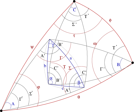
Figure 27: Left: Geometry for the intersection area of three circles of radius r centered at the three black points. Angles shown in the figure are used in equation B.2 to compute the intersection area, which is directly related to $P(\psi,\theta,\phi)$. Right: Representation of how to obtain the intersection area from sectors of spherical circles and spherical triangles.

When the intersection does not exist $P(\psi,\theta,\phi)=0$. This is the case if $r<\rho_{o}$, where $\rho_{o}$ is the radius of the spherical circumference that circumscribes the triangle $\Delta(\psi,\theta,\phi)$. It can be shown that,

$$sin(\rho_{o})=2\frac{\sin(\psi/2)\sin(\theta/2)\sin(\phi/2)}{\sqrt{(S(S-\sin(\psi/2)(S-\sin(\theta/2)(S-\sin(\phi/2)}}$$ (60)

where $S=\sin(\psi/2)+\sin(\theta/2)+\sin(\phi/2)$ When $\rho_{o}<r$ and $\rho_{o}+r<\pi$, the intersection area, $A$, exist, and to compute it we can make use of the figures in 27 as well as spherical trigonometry formulae. The intersection area $A$ is delimited by three arcs of a circle of radius $r$. Three points mark the intersection of those arcs in the limiting region. One can contruct an spherical triangle $\Delta(a,b,c)$ having those points as vertex. This is the blue triangle in figure 27, which shows all necessary angles for this section. Figure 27 also shows how one can get the area $A$ from the triangles an sectors of circles. Following this figure the area is

$$A = [B(1-\cos(r))]-[B^{\prime}+B^{\prime}+B-\pi]+[A(1-\cos(r))]-[A^{\prime}+A^{\prime}+A-\pi]$$

$$+ [C(1-\cos(r))]-[C^{\prime}+C^{\prime}+C-\pi]+[\alpha+\beta+\gamma-\pi]$$

$$= 2\pi-\cos(r)(A+B+C)-\Sigma-\Gamma-T=2\pi-\cos(r)(2\Sigma^{\prime}-2\Gamma^{\prime}-2T^{\prime}-\varphi-\omega-\tau)-\Sigma-\Gamma-T$$

where we have applied that angles $\alpha,\beta,\gamma,A,B,C$ can be expressed as a sum of other angles. The angles left can be obtained by the spherical cosinus law. We write only three angles here, but the others can be computed in a similar way.

$$\cos(\varphi) = \frac{\cos(\phi)-\cos(\psi)\cos(\theta)}{\sin(\psi)\sin(\theta)}$$ (62)

$$\cos(\Sigma) = \frac{\cos(\psi)-\cos^{2}(r)}{\sin^{2}(r)}$$

$$\cos(\Sigma^{\prime}) = \frac{\cos(r)-\cos(\psi)\cos(r)}{\sin(\psi)\sin(r)}$$

When $\rho_{o}<r$ but $\rho_{o}+r>\pi$ the intersection of the three circles exist but we can not contruct such a triangle as in 27. The area is given by all sky exept the sum of the intersection areas of the two points complementary circles, i.e.,

$$A=4\pi-4\pi(1-P(\psi))-4\pi(1-P(\theta))-4\pi(1-P(\phi))=4\pi[P(\psi)+P(\theta)+P(\phi)-2]$$ (63)

References

- [Afshordi et al ¡2004¿] Afshordi, N. , Loh, Y., Strauss, M.A., 2004, Phys. Rev D 69, 083524
- [Afshordi ¡2004¿] Afshordi,N., 2004, Phys. Rev D 70, 083536
- [Baugh et al ¡ 2004¿] Baugh C. M., et al., 2004, MNRAS, 351, L44
- [Bean & Dore ¡ 2003¿] Bean, R. & Dore, O., 2004 PRD 69, 083503
- [Beranardeau et al ¡2002¿] Bernardeau, F. et al, 2002, Phys. Rept. 367, 1
- [Boughn et al ¡1997¿] Boughn, S.P., Crittenden R.G. & Turok 1998, New Astron., 3, 275
- [Boughn & Crittenden ¡2004¿] Boughn, S. P. & Crittenden, R. G.. 2004, Nature, 427, 45
- [Boughn & Crittenden ¡2005¿] Boughn, S.P. & Crittenden, R. G., 2005, MNRAS 360, 1013
- [Cabre et al ¡2006¿] Cabré, A.,Gaztañaga, E.,Manera, M.,Fosalba, P. & Castander, F., 2006, MNRAS,372, 23
- [Corasaniti et al ¡2005¿] Corasaniti, P.S., Giannantonio, T., Melchiorri, A. 2005, PRD, 72, 023514
- [Crittenden & Turok¡1996¿] Crittenden, R. G., Turok, N., 1996, PRL, 76, 575
- [Cooray et al ¡2004¿] Cooray, A., et al, 2004, PRD 69, 027301
- [Fosalba & Gaztañaga ¡2004¿] Fosalba, P., & Gaztañaga, E., 2004, MNRAS, 350, L37