New Constraints on Oscillations in the Primordial Spectrum of Inflationary Perturbations

Abstract

We revisit the problem of constraining steps in the inflationary potential with cosmological data. We argue that a step in the inflationary potential produces qualitatively similar oscillations in the primordial power spectrum, independently of the details of the inflationary model. We propose a phenomenological description of these oscillations and constrain these features using a selection of cosmological data including the baryonic peak data from the correlation function of luminous red galaxies in the Sloan Digital Sky Survey. Our results show that degeneracies of the oscillation with standard cosmological parameters are virtually non-existent. The inclusion of new data severely tightens the constraints on the parameter space of oscillation parameters with respect to older work. This confirms that extensions to the simplest inflationary models can be successfully constrained using cosmological data.

I Introduction

Recent data from the Wilkinson Microwave Anisotropy Probe (WMAP) Spergel:2006hy ; Hinshaw:2006ia ; Page:2006hz ; Jarosik:2006ib observations of the anisotropies of the Cosmic Microwave Background (CMB) are in excellent agreement with the predictions of inflationary cosmology. In its simplest implementation, inflation is driven by the potential energy of a single scalar field slowly rolling down the potential towards the real vacuum. Under the assumption that the potential is sufficiently flat and smooth, the resulting spectrum of density perturbations is almost scale-invariant and can be described with a power-law. In the context of this slow-roll paradigm, a number of authors have used the WMAP data and various other complementary data sets to derive bounds on the inflationary parameter space. These include constraints on specific inflationary models Alabidi:2006qa ; Martin:2006rs ; Battye:2006pk ; Savage:2006tr , the Hubble dynamics during inflation Kinney:2006qm ; Peiris:2006sj , or, in a more empirical fashion, the parameters characterising the primordial power spectrum Viel:2006yh ; Seljak:2006bg ; Finelli:2006fi ; Hamann:2006pf .

In more general classes of inflationary models, however, slow roll may be violated for a brief instant Hodges:1989dw ; Starobinsky:1992ts . In single-field inflation models, such an effect can be modelled by introducing a feature such as a kink, bump or step Adams:2001vc to the inflaton potential. A step, in particular, can be regarded as an effective field theory description of a phase transition in more realistic multi-field models Lesgourgues:1999uc , which may arise naturally in, e.g., supergravity- Adams:1997de or M-theory-inspired inflation models Ashoorioon:2006wc .

This interruption of slow-roll will leave possibly detectable traces in the primordial power spectrum. Specifically, wavelengths crossing the horizon during this fast-roll phase will be affected Leach:2000yw ; Leach:2001zf , leading to a deviation from the usual power-law behaviour at these scales. Such non-standard power spectra have been brought forward to explain the peculiar glitches in the temperature anisotropies Hunt:2004vt as well as the observed low power at the largest scales Contaldi:2003zv ; Boyanovsky:2006pm .

Step-like features in the inflaton potential will lead to a burst of oscillations in the primordial power spectrum. A particular realisation of a step potential was confronted with the data in Ref. Peiris:2003ff for fixed cosmological parameters and more generally in Ref. featureshaveafuture .

In the present work, we extend the analysis of featureshaveafuture in several important aspects. Firstly, we generalise our method to spectra corresponding to a whole class of step-inflation models with arbitrary (slow-roll) background inflaton potentials. This allows us to derive constraints on parameters characterising the feature in a more model-independent way. Secondly, we address the question of parameter degeneracies: could the presence of a feature bias our estimates for the values and errors of the cosmological parameters, such as the baryon or dark matter density, in any way? Thirdly, we consider new data-sets: apart from CMB and matter power spectrum data sets, we consider also the measurements of the position of acoustic peak in the real space two-point galaxy correlation function data (BAO) from the luminous red galaxy (LRG) sample of the Sloan Digital Sky Survey (SDSS) eisenstein . This data is, in principle, especially well suited to constraining (or detecting) small amplitude oscillations in the power spectrum which would show up as a peak in the correlation function. However, due to biasing and weakly non-linear structure formation, this data is difficult to interpret and we pay special attention to do it carefully.

The paper is organised as follows: In Sec. II, we briefly remind the reader of the exact formalism of calculating the power spectrum from a given inflaton potential and compare it with the slow-roll approximation. In Sec. III, we discuss the dynamics of the inflaton field rolling over a step and introduce a generalised step model. Section IV is dedicated to our analysis methods with an emphasis on the determination of the likelihood for the BAO data set. We present our results in Sec. V, and, finally, draw our conclusions in Sec. VI.

II Inflationary Perturbations

Let us start this section with a brief recapitulation of how to calculate the primordial spectrum of curvature perturbations $\mathcal{P_{R}}$, using the formalism of Stewart and Lyth Stewart:1993bc .

In the following, we will set $c=\hbar=8\pi G=1$. We consider the gauge invariant Mukhanov variable $u$ Mukhanov:1988jd ; Sasaki:1986hm given in terms of the curvature perturbation $\mathcal{R}$:

$$u\equiv-z\mathcal{R}.$$ (1)

Here, $z\equiv a\dot{\phi}/H$, where $a$ is the scale factor, $\phi$ the inflaton field, $H$ the Hubble parameter and the dot represents a derivative with respect to time $t$. The Fourier components of $u$ obey the equation

$$u_{k}^{\prime\prime}+\left(k^{2}-\frac{z^{\prime\prime}}{z}\right)u_{k}=0,$$ (2)

with a prime denoting a derivative with respect to conformal time $\tau$.

Finally, we can define the primordial power spectrum of curvature perturbations $\mathcal{P_{R}}(k)$ via the two-point correlation function

$$\langle\mathcal{R}_{k_{1}}\mathcal{R}_{k_{2}}^{*}\rangle=\frac{2\pi^{2}}{k^{3}}\mathcal{P_{R}}(k)\;\delta^{(3)}(k_{1}-k_{2}).$$ (3)

Assuming gaussianity and adiabaticity, this quantity contains all the necessary information for a complete statistical description of the fluctuations. It is related to $u_{k}$ and $z$ via

$$\mathcal{P_{R}}(k)=\frac{k^{3}}{2\pi^{2}}\,\left|\frac{u_{k}}{z}\right|^{2}.$$ (4)

II.1 Background Equations of Motion

In order to find a solution to Equation (2), one needs to know the behaviour of the term $z^{\prime\prime}/z$. Its evolution is determined by the dynamics of the Hubble parameter and the unperturbed inflaton field, governed by Friedmann’s equation

$$H^{2}=\tfrac{1}{3}(V+\tfrac{1}{2}\dot{\phi}^{2}),$$ (5)

and the Klein-Gordon equation for $\phi$

$$\ddot{\phi}+3H\dot{\phi}+\frac{\text{d}V}{\text{d}\phi}=0.$$ (6)

For our purposes, it is convenient to introduce another time parameter, the number of $e$-foldings, defined by $N\equiv\ln a$. In terms of $N$, Equations (2), (5) and (6) read

$$H_{,\scriptscriptstyle{N}}=-\tfrac{1}{2}H\phi_{,\scriptscriptstyle{N}}^{2},$$ (7)

$$\phi_{,\scriptscriptstyle{NN}}+\left(\frac{H_{,\scriptscriptstyle{N}}}{H}+3\right)\phi_{,\scriptscriptstyle{N}}+\frac{1}{H^{2}}\frac{\text{d}V}{\text{d}\phi}=0,$$ (8)

$$u_{k,\scriptscriptstyle{NN}}+\left(\frac{H_{,\scriptscriptstyle{N}}}{H}+1\right)u_{k,\scriptscriptstyle{N}}+\left[\frac{k^{2}}{e^{2(N-N_{0})}H^{2}}\vphantom{\left(\frac{H_{,\scriptscriptstyle{N}}}{H}\right)^{2}}\left(2-\vphantom{\left(\frac{H_{,\scriptscriptstyle{N}}}{H}\right)^{2}}\right.\right.$$ (9)

$$\left.\left.4\,\frac{H_{,\scriptscriptstyle{N}}}{H}\frac{\phi_{,\scriptscriptstyle{NN}}}{\phi_{,\scriptscriptstyle{N}}}-2\left(\frac{H_{,\scriptscriptstyle{N}}}{H}\right)^{2}-5\,\frac{H_{,\scriptscriptstyle{N}}}{H}-\frac{1}{H^{2}}\frac{\text{d}^{2}V}{\text{d}\phi^{2}}\right)\right]u_{k}=0,$$

with $N_{0}$ determining the normalisation of the scale factor. This coupled system of differential equations can easily be solved numerically, once a suitable set of initial conditions has been chosen.

II.2 Initial Conditions

Supposing that at a time $N_{sr}$ the system has reached the inflationary attractor solution

$$\ddot{\phi}\ll 3H\dot{\phi},$$ (10)

and is rolling slowly,

$$\dot{\phi}^{2}\ll V(\phi),$$ (11)

the initial conditions for $\phi$ and $H$ will be given by

$$\phi(N_{sr}) =\phi_{sr}$$ (12)

$$\phi_{,N}(N_{sr}) =-\frac{1}{V(\phi_{sr})}\left.\frac{\text{d}V}{\text{d}\phi}\right|_{\phi_{sr}}$$ (13)

$$\quad H(\phi_{sr}) =\sqrt{\frac{V(\phi_{sr})}{3}}.$$ (14)

The initial conditions for $u_{k}$ can be obtained by requiring the late time solution of (2) to match the solution of a field in the Bunch-Davies vacuum of de Sitter space, given by

$$u_{k}(\tau)=\frac{e^{-ik\tau}}{\sqrt{2k}}\left(1+\frac{i}{k\tau}\right),$$ (15)

at early times, well before the observationally relevant scales leave the horizon. For $k\gg z^{\prime\prime}/z$ (or, equivalently, $k\tau\gg 1$) this can be approximated by the free field solution in flat space

$$u_{k}=\frac{1}{\sqrt{2k}}\,e^{-\mathrm{i}k\tau}.$$ (16)

Fixing the irrelevant phase, we obtain the initial conditions for a mode $k$

$$u_{k}(\tau_{0}) =\frac{1}{\sqrt{2k}},$$ (17)

$$u_{k}^{\prime}(\tau_{0}) =-i\sqrt{\frac{k}{2}}$$ (18)

at a time $\tau_{0}$ satisfying $k\gg z^{\prime\prime}/z|_{\tau_{0}}$.

II.3 Slow Roll

Following Ref. Liddle:1994dx , we define the Hubble slow roll parameters by

$${}^{n}\!\beta_{H}\equiv\left\{\prod^{n}_{i=1}\left[-\frac{\text{d}\ln H^{(i)}}{\text{d}\ln a}\right]\right\}^{1/n}=2\left(\frac{(H^{(1)})^{n-1}H^{(n+1)}}{H^{n}}\right)^{1/n}$$ (19)

for $n\geq 1$, with a superscript “$(n)$” denoting the $n\text{th}$ derivative with respect to $\phi$. In addition to that, we define ${}^{0}\!\beta_{H}\equiv 2(H^{(1)}/H)^{2}$. The first three parameters of the Hubble slow roll hierarchy read

$$\epsilon_{H} \equiv\;^{0}\beta_{H}=2\left(\frac{H^{(1)}(\phi)}{H(\phi)}\right)^{2}=-\frac{\dot{H}}{H^{2}},$$ (20)

$$\eta_{H} \equiv\;^{1}\beta_{H}=\;\frac{H^{(2)}(\phi)}{H(\phi)}=-\frac{\ddot{\phi}}{\dot{\phi}H},$$ (21)

$$\xi^{2}_{H} \equiv(^{2}\!\beta_{H})^{2}=2\;\frac{H^{(1)}(\phi)H^{(3)}(\phi)}{H^{2}(\phi)}=\frac{\stackrel{{\scriptstyle...}}{{\phi}}}{2H^{2}\dot{\phi}}-\tfrac{1}{2}\eta_{H}^{2}.$$ (22)

Using these definitions it can be shown that the mode equation (2) can be written as

$$u_{k}^{\prime\prime} +\left(k^{2}-2a^{2}H^{2}\left[1+\epsilon_{H}-\tfrac{3}{2}\eta_{H}+\epsilon_{H}^{2}-\vphantom{\frac{1}{2}}\right.\right.$$ (23)

$$\left.\left.2\epsilon_{H}\eta_{H}+\tfrac{1}{2}\eta_{H}^{2}+\xi_{H}^{2}\right]\vphantom{\frac{1}{1}}\right)u_{k}=0.$$

Note that this expression is exact: it does not assume the slow roll parameters to be small.

From a model-building point of view, where one regards the Lagrangian (or the scalar potential) of the theory as the fundamental quantity, the calculation of the Hubble slow roll parameters can be quite involved. In this sense it may be more convenient to work with the potential slow roll parameters instead, which use derivatives of the potential instead of derivatives of the Hubble parameter. The first three potential slow roll parameters are defined by

$$\epsilon \equiv\tfrac{1}{2}\left(\frac{V^{(1)}}{V}\right)^{2},$$ (24)

$$\eta \equiv\frac{V^{(2)}}{V},$$ (25)

$$\xi^{2} \equiv\frac{V^{(1)}V^{(3)}}{V^{2}}.$$ (26)

If the attractor condition (Eq. (10)) is satisfied, the two are approximately related via Liddle:1994dx

$$\epsilon_{H} =\epsilon-\tfrac{4}{3}\epsilon^{2}+\tfrac{2}{3}\epsilon\eta+\mathcal{O}(3),$$ (27)

$$\eta_{H} =\eta-\epsilon+\tfrac{8}{3}\epsilon^{2}+\tfrac{1}{3}\epsilon\eta+\tfrac{1}{3}\xi^{2}+\mathcal{O}(3),$$ (28)

$$\xi^{2}_{H} =\xi^{2}-3\epsilon\eta+3\epsilon^{2}+\mathcal{O}(3),$$ (29)

up to corrections of third and higher orders. Expressed in terms of the potential slow roll parameters, $z^{\prime\prime}/z$ is given by

$$\frac{z^{\prime\prime}}{z}= 2a^{2}H^{2}\left[1+\tfrac{5}{2}\epsilon-\tfrac{3}{2}\eta+\tfrac{7}{6}\epsilon^{2}-\right.$$ (30)

$$\left.\tfrac{35}{6}\epsilon\eta+\tfrac{1}{2}\eta^{2}+\tfrac{1}{2}\xi^{2}+\mathcal{O}(3)\right]$$

It is commonly assumed that the first two slow roll parameters vary slowly with time (i.e., $\xi_{(H)}^{2}\ll 1$). Then it follows that, if one wants to sustain inflation for long enough to solve the horizon and flatness problems, $\epsilon_{(H)}$ and $|\eta_{(H)}|$ will also have to be much smaller than unity. In this (“slow roll”) limit, we have $z^{\prime\prime}/z\approx 2a^{2}H^{2}$, $\dot{H}\approx 0$ and $a\propto\exp[Ht]$.

Let us now turn back to Eq. (2), which is basically the equation of an oscillator with a time dependent mass term, and discuss its solutions. The initial conditions imply that for wavenumbers with

$$\frac{k}{a}\gg H,$$ (31)

i.e., with wavelengths much smaller than the horizon, the solution is given by Equation (16) and $u_{k}$ describes a circular motion in the complex plane. Due to the exponential growth of the scale factor, the physical wavelenghts will be blown up and leave the horizon, eventually satisfying $k/a\ll H$. In this limit, the growing solution for $u_{k}$ is given by

$$u_{k}\propto z.$$ (32)

Hence, the spectrum $\mathcal{P_{R}}$ will converge to a constant value for super-Hubble modes, i.e., the perturbations “freeze in”. We can also conclude that the fate of a perturbation with wavelength $k$ is decided when $k/a\sim H$ and the spectrum will have its final shape imprinted on horizon exit. It is not until much later, when the modes reenter the horizon during radiation or matter domination, that they will exhibit dynamical behaviour again.

Generically, the power spectrum will not be scale independent, with a scale dependence being induced by the variation of, e.g., the potential energy and the Hubble parameter as the inflaton field rolls down the potential. In the slow roll regime, however, the scale dependence is rather weak and $\mathcal{P_{R}}$ can be reasonably well approximated by a power law:

$$\mathcal{P_{R}}(k)\simeq A_{\text{S}}\left(\frac{k}{k_{0}}\right)^{n_{\text{S}}-1},$$ (33)

with the normalisation $A_{\text{S}}$ given by

$$A_{\text{S}}\simeq\left.\frac{1}{24\pi^{2}}\frac{V}{\epsilon}\right|_{k_{0}=aH},$$ (34)

and the spectral index

$$n_{\text{S}}\simeq 1-6\epsilon+2\eta.$$ (35)

Before we talk about relaxing some of the assumptions that went into this analysis, let us quickly mention inflationary tensor perturbations.

II.4 Tensor Perturbations

Apart from the scalar perturbations described above, inflation also generates tensor perturbations, with a spectrum given by

$$\mathcal{P}_{\text{grav}}(k)=\frac{k^{3}}{2\pi^{2}}\left|\frac{v_{k}}{a}\right|^{2}$$ (36)

and the mode equation

$$v_{k}^{\prime\prime}+\left(k^{2}-\frac{a^{\prime\prime}}{a}\right)v_{k}=0.$$ (37)

This equation is very similar to the scalar one. This similarity can be readily seen if we express the “mass term” $a^{\prime\prime}/a$ in terms of the slow roll parameters:

$$\frac{a^{\prime\prime}}{a} =2a^{2}H^{2}\left[1-\tfrac{1}{2}\epsilon_{H}\right]$$ (38)

$$\simeq 2a^{2}H^{2}\left[1-\tfrac{1}{2}\epsilon+\tfrac{2}{3}\epsilon^{2}-\tfrac{1}{3}\epsilon\eta+\mathcal{O}(3)\right].$$

Just like the scalar modes, tensor perturbations will also freeze in at horizon exit. In the slow roll case their spectrum is approximately

$$\mathcal{P}_{\text{grav}}(k)\simeq A_{\text{T}}\left(\frac{k}{k_{0}}\right)^{n_{\text{T}}},$$ (39)

with the tensor spectral index

$$n_{\text{T}}\simeq-2\epsilon,$$ (40)

and normalisation

$$A_{\text{T}}\simeq\left.\frac{2}{3\pi^{2}}V\right|_{k_{0}=aH}.$$ (41)

III Slow Roll Interrupted

The validity of the power-law parameterisation of the primordial spectra rests on the assumptions that the slow-roll parameters are small and change slowly with time. Let us relax the latter and allow $\epsilon$ and $\eta$ to change significantly on a timescale $\Delta N\lesssim 1$. This has the consequence that we can also allow $\epsilon$ and/or $\eta$ to become of order unity momentarily, provided that at a later time, the system returns to the slow roll regime. We also assume here that the system starts in a state where the slow roll conditions are fulfilled, in order to give it enough time to reach the inflationary attractor solution.

This effect can be modelled by adding a local feature, such as a step or a bump, to an otherwise flat inflaton potential.

III.1 Chaotic Inflation Step Model

Let us examine the consequences of such a feature using as an example the same model potential as in featureshaveafuture

$$V(\phi)=\tfrac{1}{2}\,m^{2}\phi^{2}\,\left(1+c\tanh\left(\frac{\phi-b}{d}\right)\right).$$ (42)

This potential describes standard $m^{2}\phi^{2}$ chaotic inflation Linde:1983gd with a step centered around $\phi=b$. The height of the step is determined by $c$, its gradient by $d$. We do not want inflation to be interrupted by the step, so we stipulate $|c|\ll 1$ to ensure that the potential energy will always dominate over the kinetic one.

As pointed out above, the eventual spectrum crucially depends on the dynamics of $z^{\prime\prime}/z$, which can easily be deduced from the solution of Equations (7) and (8). For a typical choice of parameters, we plot the numerical solution in Figure 1. Generically, we find that $z^{\prime\prime}/(za^{2}H^{2})$ has a maximum before the inflaton field reaches $b$, a minimum shortly afterwards and it will return to the asymptotic slow roll value of $\sim 2$ after $\mathcal{O}(1)$ $e$-folding. Comparison with the Hubble slow roll parameters (Fig. 1) shows that this behaviour is mainly caused by $\eta_{\text{H}}$ and $\xi^{2}_{\text{H}}$, while $\epsilon_{\text{H}}$ remains small. This is a consequence of the condition $c\ll 1$. Beware that the potential slow roll approximation Eq. (30) will in general not work for this potential since the contribution of higher derivative terms can be large. The smallness of $\epsilon_{H}$ (and hence $\epsilon$) also implies that there will not be any sizable deviations from a power law for the spectrum of tensor perturbations.

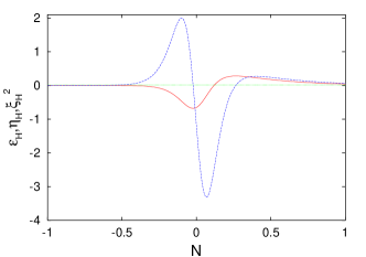
Figure 1: Top: $z^{\prime\prime}/z$ divided by $a^{2}H^{2}$ for $b=14$, $c=10^{-3}$ and $d=2\times 10^{-2}$ versus the number of $e$-foldings. $N$ is set to zero for $\phi=b$. It takes the inflaton field roughly half an $e$-folding to roll over the step.
Bottom: Hubble slow roll parameters at the step, $\epsilon_{\text{H}}$ (dotted green line) remains negligible throughout, while $\eta_{\text{H}}$ (solid red line) and $\xi^{2}_{\text{H}}$ (dashed blue line) violate the slow roll conditions.

So, how will this particular behaviour of $z^{\prime\prime}/z$ influence the solution for $u_{k}$ and eventually the spectrum compared to a model with no step? It is obvious that modes with $k^{2}\gg\text{Max}|z^{\prime\prime}/z|$, i.e., modes that are well within the horizon at the time of the step, will not be affected at all and $u_{k}$ will remain in the oscillatory regime. For $k^{2}\lesssim\text{Max}|z^{\prime\prime}/z|$, the maximum in $z^{\prime\prime}/z$ will result in a boost of exponential growth for $u_{k}$, reverting to oscillations when $z^{\prime\prime}/z$ goes negative and eventually return to the growing solution. We depict the motion of $u_{k}$ in the complex plane in Fig. 2.

Figure 2: These figures show the evolution of $u_{k}$ in the complex plane, where $u_{k}$ has been normalised to one in the oscillating limit. The choice of initial conditions (17,18) ensures that the motion will be initially circular. The top left plot shows a mode that is not affected by the feature, so that the circular oscillation goes straight into a growing motion. In the other two plots the circle gets deformed by an intermittent phase of growth triggered by the peak of $\tfrac{z^{\prime\prime}}{z}$, to be followed by another phase of elliptic oscillations (caused by the dip of $\tfrac{z^{\prime\prime}}{z}$) until finally the modes leave the horizon and start growing. Whether a mode is suppressed or enhanced by this mechanism depends on the phase of the oscillation when the growth sets in. Growth along the semi-major axis will lead to an enhancement (top right), whereas growth along the semi-minor axis entails a suppression (bottom) with respect to the modes of the corresponding featureless model.

When an oscillatory phase is preceded by a growing phase, the initial circle will be distorted to an ellipse. As the growth sets in again, the the mode will be suppressed or enhanced, depending on the phase of the oscillation, which itself is $k$-dependent. In the spectrum, this can be observed as oscillations. This mechanism will be most effective for modes that are just leaving the horizon, for modes with $k^{2}\ll\text{Max}|z^{\prime\prime}/z|$ the phase difference will be negligible.

Hence, a localised feature in the potential will lead to a localised “burst” of oscillations in the spectrum (see also Ref. Burgess:2002ub ), while large and small scales will remain unchanged with respect to the spectra of the asymptotic background models. This is shown in Fig. 3.

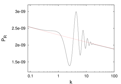
Figure 3: Primordial power spectrum for a model with $m=7.5\times 10^{-6}$, $b=14$, $c=10^{-3}$ and $d=2\times 10^{-2}$ (solid black line) with wavenumber $k$ given in units of $aH|_{\phi=b}$. The dotted red line depicts the spectrum of the same model with $c$ set to zero.

Note that the wavelengths affected by the feature are those that are about to leave the horizon as the inflaton field reaches the centre of the step. In particular, also the frequency of the oscillations of the spectrum is proportional to this scale.

What remains is to identify the horizon size at the step with a physical scale today. This connection can be made if one knows the total number of $e$-foldings $N_{*}$ of inflation that took place after a known physical scale $k_{*}$ left the horizon. Technically, we evolve the background equations (7,8) until the end of inflation $N_{\text{end}}$, (defined by $\ddot{a}(N_{\text{end}})=0$). The scale $k_{*}$ can then be determined in units of $aH|_{\phi=b}$ via

$$k_{*}\leftrightarrow\frac{a(N_{\text{end}}-N_{*})\;H(N_{\text{end}}-N_{*})}{aH|_{\phi=b}}.$$ (43)

As long as the spectrum of the $c=0$ background model is only mildly scale dependent, there will be a strong degeneracy between $N_{*}$ and $b$: shifting the feature in the potential will have the same effect as shifting the scale of $k$. In the following we will therefore not treat $N_{*}$ as a free parameter, but set $N_{*}=50$ for $k_{*}=0.05\;h\,\text{Mpc}^{-1}$. If we want the feature to affect scales that are within reach of current observations, this will require $b$ to lie in the interval $14\lesssim b\lesssim 15$.

III.2 Model Dependence

Having analysed a specific example in the previous subsection, let us now address the question of model dependence: Will we arrive at different conclusions if we modify the background inflationary model (e.g., $\lambda\phi^{4}$ instead of $m^{2}\phi^{2}$) or the parameterisation of the step?

We will argue that a more general potential

$$V(\phi)=V_{0}+f(\phi)\;S(\phi-b)$$ (44)

leads to a qualitatively similar spectrum as the potential (42). Here, $V_{\text{bg}}(\phi)\equiv V_{0}+f(\phi)$ is the background potential, which should fulfil the slow roll conditions with $f$ and $V_{0}$ positive definite. The function $S(\phi)$ parameterises the step, and should monotonically asymptote to $1\pm c$ ($c\ll 1$) for $\phi\gg b$ and $\phi\ll b$, respectively, with $S(0)=1$.

As we have seen above, the derivatives of the potential are crucial to determining the spectrum. In general, the derivatives of $V$ are given by

$$V^{(n)}(\phi)=\sum_{i=0}^{n}\binom{n}{i}f^{(i)}(\phi)\;S^{(n-i)}(\phi).$$ (45)

Far away from the step, the derivatives of $S$ will be negligible and the potential and its derivatives are approximately

$$V(\phi)\simeq V_{0}+f(\phi)(1\pm c)\simeq V_{\text{bg}}(\phi),$$ (46)

$$V^{(n)}(\phi)\simeq f^{(n)}(\phi)(1\pm c)\simeq V_{\text{bg}}^{(n)}(\phi).$$ (47)

Since the slow roll conditions hold here, the spectrum will be given by Eq. (33) with

$$A_{\text{S}} \simeq A_{\text{S}}^{\text{bg}}\left(1\pm c\left(\frac{3f}{V_{0}+f}-2\right)+\mathcal{O}(c^{2})\right),$$ (48)

$$n_{\text{S}} \simeq n_{\text{S}}^{\text{bg}}\pm c\left(\frac{2V_{0}}{V_{0}+f}\left(\eta^{\text{bg}}-6\epsilon^{\text{bg}}\right)\right)+\mathcal{O}(c^{2}).$$ (49)

In the special case $V_{0}=0$, we have exactly $A_{\text{S}}=A_{\text{S}}^{\text{bg}}(1\pm c)$ and $n_{\text{S}}=n_{\text{S}}^{\text{bg}}$. If $V_{0}\neq 0$, there are additional corrections of order $c$ to the normalisation and also corrections to the tilt, which are suppressed by $c$ and the slow-roll parameters of the background model. In both cases, one asymptotically recovers the spectrum of the background model in the limit $c\ll 1$.

Near the step, however, the derivatives of $V$ will have a contribution from the derivatives of $S$. If the step is sharp enough, the $n$th derivative of $V$ will be dominated by the $n$th derivative of $S$, since the other terms are suppressed with factors of the order of the slow roll parameters of the background model. Hence, the dynamics of $z^{\prime\prime}/z$ near the step hardly depends on the background, but is determined by the form of $S$. On the other hand, any $S$ that gives a $z^{\prime\prime}/z$ which roughly shows a behaviour like the one depicted in Fig. 1, will lead to a burst of oscillations in the power spectrum. The similarities between spectra of different background models are illustrated in Fig. 4, where we plot the spectra of a hybrid inflation type potential

$$V(\phi)=V_{0}+\tfrac{1}{2}\,m^{2}\phi^{2}\,\left(1+c\tanh\left(\frac{\phi-b}{d}\right)\right),$$ (50)

and another monomial potential with a different form of the step function

$$V(\phi)=\lambda\,\phi^{4}\,\left(1+c\arctan\left(\frac{\phi-b}{d}\right)\right).$$ (51)

Note that despite the difference in background models and step functions, the maxima and minima of the oscillations occur at the same wavelengths.

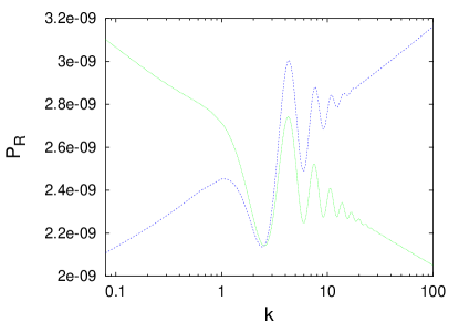
Figure 4: Primordial power spectra of a hybrid inflation type step model (50) with $V_{0}=3.7\times 10^{-14}$, $m=3.2\times 10^{-8}$, $b=0.0125$, $c=10^{-3}$ and $d=5\times 10^{-5}$ (dashed blue line), and of potential (51) with parameters $\lambda=6\times 10^{-14}$, $b=21$, $c=5\times 10^{-4}$ and $d=0.02$ (dotted green line). The hybrid inflation background model has $n_{\text{S}}>1$, suppressing large scale fluctuations, while the $\lambda\phi^{4}$ model has $n_{\text{S}}<1$ with more power on large scales.

To alleviate the model dependence of the analysis when confronting theory with experiment, we choose a phenomenological approach and define the spectrum of a generalised step model

$$\mathcal{P_{R}}^{\text{gsm}}=\mathcal{P_{R}}^{\text{step}}\left(\frac{k}{k_{0}}\right)^{n_{\text{S}}-n_{\text{S}}^{\text{step}}}.$$ (52)

Here, $\mathcal{P_{R}}^{\text{step}}$ is the spectrum obtained from the potential Eq. (42) and $n_{\text{S}}^{\text{step}}=0.96$ is the spectral index of the $\tfrac{1}{2}m^{2}\phi^{2}$ model. The quantity $n_{\text{S}}$ then describes the overall effective tilt of the spectrum. Spectra of this type will arise from potentials of the form Eq. (44). While the fine details of particular models may differ slightly from this approximation, Eq. (52) will nevertheless capture the broad features of a large class of background models, since, as argued above, the shape of the burst of oscillations is largely independent of the background model. Minor differences would likely be washed out in the angular power spectrum of the CMB anyway Kawasaki:2004pi . The asymptotic behaviour of models with $V_{0}=0$ will be reproduced exactly; for $V_{0}>0$ it will be approximate, with errors of order $c$.

There is a catch however: in this analysis the parameters $b$, $c$ and $d$ will be bereaved of their meaning as parameters of the potential. Instead, they should be interpreted as phenomenological parameters which describe the spectrum. This does not preclude us from deriving meaningful constraints, though. We argued that the shape of the modulation of the spectrum is largely independent of the background, so similar modulations should be the consequence of similar step dynamics. A useful quantity in this context is the maximum value the slow roll parameters $\epsilon$, $\eta$ and $\xi^{2}$ can reach at the step. For the potential (42), we can estimate $\epsilon_{\text{max}}$, $\eta_{\text{max}}$ and $\xi^{2}_{\text{max}}$ in terms of $b$, $c$ and $d$:

$$\epsilon_{\text{max}} \simeq\epsilon^{\text{bg}}+\frac{c^{2}}{2d^{2}}+\frac{2c}{bd},$$ (53)

$$\eta_{\text{max}} \simeq\eta^{\text{bg}}+0.77\frac{c}{d^{2}},$$ (54)

$$|\xi^{2}_{\text{max}}| \simeq 2\frac{c^{2}}{d^{4}}+4\frac{c}{bd^{3}},$$ (55)

assuming $c<1$, $d<1$ and $b>1$. Note that $\xi^{2}=0$ for the background model.

Along the same lines, one can can replace $b$ with $k_{\text{s}}$, corresponding to today’s wavenumber of the perturbations that left the horizon during inflation when $\phi=b$.

IV Data Analysis

We compare the theoretical predictions of three theoretical models (A, B and C) with observational data. We use the Markov chain Monte Carlo (MCMC) package cosmomc cosmomc to reconstruct the likelihood function in the space of model parameters and infer constraints on these parameters.

IV.1 Models

The three models have four parameters in common: $\omega_{b}$ (baryon density), $\omega_{c}$ (CDM density), $\tau$ (optical depth to reionisation) and $\theta_{s}$ (sound horizon/angular diameter distance at decoupling). The difference lies in the primordial power spectrum.

• Vanilla power-law $\Lambda$CDM model: the initial spectrum is parameterised with $A_{\text{S}}$ and $n_{\text{S}}$.

• Step model (Eq. (42)) with parameters $A_{\text{S}}$, $b$, $c$ and $d$.

• Generalised step model, which uses an effective tilt $n_{\text{S}}$ in addition to the parameters of model B. Constraints on $\epsilon_{\text{max}}-\epsilon^{\text{bg}}$, $\eta_{\text{max}}-\eta^{\text{bg}}$ and $\xi^{2}_{\text{max}}$ are derived using Eqns. (53)-(55).

We limit our analysis to scalar perturbations. While tensor perturbations may, in principle, give a subdominant contribution, their spectrum will be smooth in the class of models studied here, so we do not expect any major degeneracies with the step parameters.

IV.2 Data Sets

To assess the influence of different data on the constraints, we perform the analysis for each of the models using three different sets of data:

• WMAP three year temperature and polarisation anisotropy dataSpergel:2006hy ; Hinshaw:2006ia ; Page:2006hz ; Jarosik:2006ib (WMAP3). The likelihood is determined using the October 2006 version of the WMAP likelihood code available at the LAMBDA website lambda .

• WMAP3 plus small scale CMB temperature anisotropy data from the ACBAR acbar , BOOMERANG boomerang and CBI cbi experiments, plus the power spectrum data of the luminous red galaxy sample from the Sloan Digital Sky Survey (SDSS), data release 4 Tegmark:2006az . To avoid a dependence of our results on nonlinear modelling, we only use the first 13 $k$-bands ($k/h<0.09$ Mpc^-1).

• Same as data set 2, plus two-point correlation function data from the SDSS LRG eisenstein .

IV.3 Analysis

Our constraints are derived from eight parallel chains generated using the Metropolis algorithm Metropolis:1953am . We use the Gelman and Rubin $R$ parameter gelru to keep track of convergence of the chains, stopping the chains at $R-1<0.05$. Since the likelihood function is highly nongaussian in some parameter directions and even multimodal in certain cases, we double-check our results by comparing with chains generated with a variation of the multicanonical sampling algorithm Berg:1998nj .

IV.4 Priors

Apart from the hard-coded priors of cosmomc on $H_{0}$ ($40$ km/s/Mpc $<H_{0}<100$ km/s/Mpc) and the age of the Universe ($10^{10}$ a $<A<2\times 10^{10}$ a), we impose flat priors on the other cosmological parameters. For the parameters of the potential we choose a flat prior on $b\in[14,15]$ and logarithmic priors on $c,d$ and $c/d^{2}$ ($\log c\in[-6,-1]$, $\log d\in[-2.5,-0.5]$, $\log c/d^{2}\in[-5,3]$).

IV.5 Baryon Acoustic Peak

Oscillations in the dark matter power spectrum due to acoustic oscillations in the plasma prior to decoupling result in an single peak in the two-point correlation function of the distribution of galaxies $\xi(r)$. In Ref. eisenstein , the authors claim the detection of such a peak and identify it as corresponding to the baryonic oscillations of the matter power spectrum.
Since any oscillation of the spectrum, regardless of its origin, will lead to a feature in the correlation function, this data set is particularly well suited to constraining oscillations in the initial power spectrum as well, provided that the features are not completely washed out through subsequent evolution.

The correlation function is related to the matter power spectrum $P(k)$ via a Fourier transform:

$$\xi(r)\propto\int_{0}^{\infty}\text{d}k\,k^{2}P(k)\frac{\sin kr}{kr}.$$ (56)

Technically, the upper limit of the integral would be some ultraviolet cutoff $k_{UV}$, chosen such that the error in $\xi$ is small ($\ll 1\%$). For the scales covered by the SDSS data, i.e., comoving separations between 12 and 175 $h^{-1}\text{Mpc}$, this requires a momentum cutoff $k_{UV}>1\,h/\text{Mpc}$. At these wavenumbers, however, nonlinear effects cannot be neglected anymore, which makes the theoretical prediction of $\xi$ somewhat tricky.

The standard procedure is outlined in section 4.2 of Ref. eisenstein and involves corrections for redshift space distortion, nonlinear clustering, scale dependent bias, and a smoothing of features on small scales due to mode coupling. All of these methods were calibrated with nonlinear simulations in a vanilla cosmology setting and it is not obvious that they should be applicable to our case. With the exception of the smoothing, however, the effect of these corrections on the correlation function is smaller than 10% and will only be noticable at scales $<40h^{-1}$ Mpc (see Figure 5 of eisenstein ). So even if we assume a large uncertainty in the nonlinear corrections, the accuracy of the theoretical correlation function will still be of order a few per cent, that is smaller than the error bars of the data.

Let us look at the smoothing procedure in a bit more detail. In the usual case, the dewiggled transfer function $T_{\text{dw}}$ is a weighted interpolation between the linear transfer function $T_{\text{lin}}$ and the Eisenstein-Hu eihu no-wiggle transfer function $T_{\text{nw}}$

$$T_{\text{dw}}(k)=w(k)\,T_{\text{lin}}(k)+\left(1-w(k)\right)\,T_{\text{nw}},$$ (57)

with a weight function $w(k)=\exp\left[-(ak)^{2}\right]$ and $a=7h^{-1}$ Mpc. This is related to the dewiggled spectrum by

$$P_{\text{dw}}(k)=k\,T_{\text{dw}}^{2}(k)\,\mathcal{P_{R}}(k).$$ (58)

In the case of a non-smooth primordial power spectrum $\mathcal{P_{R}}(k)$, one should of course also dewiggle the initial features. In order to recover the standard procedure for power-law spectra, we will instead smooth the quantity

$$\hat{T}(k)\equiv\left(P(k)/k\right)^{1/2}=T(k)\sqrt{\mathcal{P_{R}}(k)}.$$ (59)

The use of the no-wiggle transfer function rests on the assumption that at small scales, mode coupling will totally erase all structure, which is reasonable as long as the amplitude of features is of the same order as that of the baryon oscillations. For much larger oscillations, mode coupling might not be efficient enough to erase all structure; it is likely that some residual oscillations will remain. So instead of a no-wiggle $\hat{T}_{\text{nw}}$, we will use a smoothed $\hat{T}_{\text{s}}$ defined by

$$\hat{T}_{\text{s}}(k,q)=\exp\left[\frac{1}{q}\int_{\ln k-q/2}^{\ln k+q/2}\text{d}\!\ln\!k^{\prime}\,\ln\left[\hat{T}_{\text{lin}}(k^{\prime})\right]\right],$$ (60)

i.e., a convolution of $\hat{T}_{\text{lin}}$ with a top hat function of width $q$ in log-log space. The dewiggled power spectrum is then given by

$$P_{\text{dw}}(k,q)=k\left(w(k)\,\hat{T}_{\text{lin}}(k)+\left(1-w(k)\right)\,\hat{T}_{\text{s}}(k,q)\right)^{2}.$$ (61)

Without turning to $N$-body simulations it would be hard to estimate how much the spectrum will have to be smoothed, though. Therefore, we will determine the BAO likelihood $\mathcal{L}_{\text{BAO}}$ by marginalising over $q$:

$$\mathcal{L}_{\text{BAO}}=\int\text{d}q\,\mathcal{L}(q)\pi(q).$$ (62)

V Results

An important question in the context of a model-dependent analysis is how the choice of model will affect the estimates of the parameters, particularly if the models are nested. Possible degeneracies between “standard” and newly introduced parameters can bias means as well as errors. In Fig. 5, we plot the marginalised likelihood distributions for the vanilla parameters for all three models with data set 1. There are small differences between models A and B for $\Omega_{b}h^{2}$, $\tau$ and the normalisation. These arise due to the fact that in model B, the tilt of the spectrum is fixed. There is a well-known degeneracy between these parameters and the spectral index. Fixing the tilt near the best fit value will reduce the errors on the parameters it is degenerate with, which is precisely what is happening here.

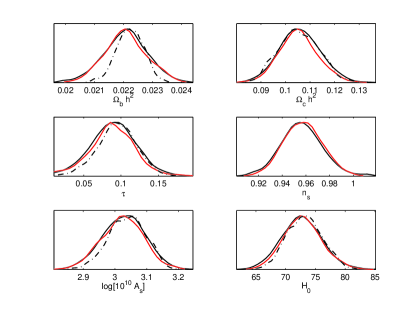
Figure 5: Marginalised likelihoods for model A (solid red line), model B (dot-dashed line) and model C (solid black line). The differences between the results for A and C are marginal. For some parameters, the results for model B differ slightly. This should be attributed to the degeneracies of the spectral index with these parameters and the fact that the tilt of the spectrum is fixed in this model, it is not due to the presence of a feature.

The distributions for models A and C show a remarkable similarity which leads us to conclude that the presence of a feature will not have any statistically significant influence on the results for the parameters of the vanilla model. This conclusion remains unchanged if we consider the other data sets.

Another interesting question is whether the data prefer the presence of a feature over a smooth spectrum. How much will a feature improve the fit and can we understand why?

In Ref. featureshaveafuture , we studied model B and found two regions in parameter space which improve the fit to the WMAP3 data by $\Delta\chi^{2}\sim 5$ and $\Delta\chi^{2}\sim 7$, respectively. The former corresponds to oscillations at large scales ($\ell\simeq 20-30$), while the latter has oscillations of a wavelength similar to the baryonic acoustic oscillations and lies near the third peak of the CMB temperature power spectrum. Adding small scale CMB data and, in particular, the power spectrum data of the 2003 data release of the SDSS Tegmark:2003uf , improved the fit of the small scale maximum to $\Delta\chi^{2}\sim 15$.

In the present work, we replaced the old main sample data with the luminous red galaxy sample of the most recent SDSS data release. With this newer data set, however, we do not find such an enhancement of the $\Delta\chi^{2}$ anymore. In fact, it appears to disfavour a large feature near the third peak. Given the better quality of the LRG power spectrum data and the fact that the BAO data also does not seem to support this effect, it is likely that the improvement in the fit was just a fluke. The disappearance of this maximum of the likelihood function is illustrated in Fig. 6, where we show the mean likelihood (colour-coded) and the 99% confidence level of the marginalised likelihood in the ($b,\log c$) plane of parameter space. The inclusion of large scale structure data and BAO data considerably tightens the constraints on features at small scales corresponding to values of $b$ between $\sim\!14.1$ and $\sim\!14.4$, while for larger values of $b$, i.e., features at larger scales, the contours remain roughly the same.

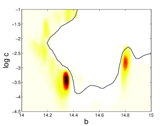
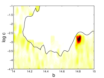
Figure 6: 99% confidence level contours for model B in the ($b$, $\log c$) plane of parameter space with data sets 1 (top), 2 (centre) and 3 (bottom). In these directions of parameter space, the likelihood function has a plateau towards vanishing step heights where the model reduces to the featureless $m^{2}\phi^{2}$ case, an excluded valley corresponding to large steps and a peak at $b\simeq 14.8$. For the WMAP data alone we also find a second peak near $b\simeq 14.3$.

The feature at large scales ($b\simeq 14.8$), on the other hand, remains untouched when we add the small scale data sets. For the generalised step model and data set 1, the large scale feature maximum likelihood point is at ($b=14.8$, $c=0.001$, $d=0.02$, $\Omega_{b}h^{2}=0.0216$, $\Omega_{c}h^{2}=0.102$, $\tau=0.11$, $n_{\text{S}}=0.952$, $\log[10^{10}A_{\text{S}}]=3.05$ and $H_{0}=72.7$), which lies near the maximum of the marginalised 1D likelihoods of the vanilla model in Fig. 5. This is a further indication that the presence of a feature at large scales will not affect the estimates of the other parameters.

Going from model B to the generalised step model will slightly improve the quality of the fits, yielding an extra $\Delta\chi^{2}$ of 1-2. We did not expect a major improvement here, since the spectral tilt of the $m^{2}\phi^{2}$ model lies fairly close to the best fit value of the vanilla model with a freely varying $n_{\text{S}}$.

In Fig. 7, we show the marginalised and mean likelihoods for the wavenumber $k_{\text{s}}$ of the perturbations that left the horizon when the inflaton field passed the step (i.e., at the moment when $\phi=b$). Again, we can see how the inclusion of the data sets sensitive to smaller scales reduces the evidence for a feature at scales $\gtrsim\mathcal{O}(10^{-2})\;\text{Mpc}^{-1}$. The difference between the mean and marginalised likelihoods is due to a volume effect: integration over the low $c$ plateau of the likelihood function tends to suppress peaks in the marginalised likelihood, which show up more clearly in the mean likelihood.

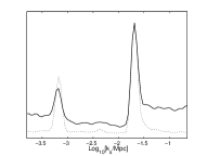
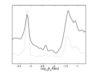
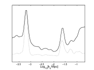
Figure 7: Marginalised (solid line) and mean likelihoods (dotted line) for parameter $k_{\text{s}}$ in the generalised step model, indicating at which wavelengths a feature is likely to happen. Top left: data set 1, top right: data set 2, bottom: data set 3.

Finally, we display constraints on the maximum values of the slow roll parameters of the step function in Fig. 8. While the WMAP3 data alone is only sensitive to features up to a wavelength of $\sim 10^{-2}\;\text{Mpc}^{-1}$, the large scale structure data extends the sensitivity by almost a factor ten in $k$. We find fairly strong bounds on the maximum value of $\epsilon$ for the step function. In conjunction with Eq. (38), this implies that the spectrum of tensor perturbations is unlikely to experience an oscillatory modulation like the scalar spectrum, since that would require $\epsilon$ to be of order one.

For the higher order slow roll parameters, values up to a few (for $\eta$) and up to a few hundred (for $\xi^{2}$) are still allowed. Note, however, that these bounds are parameterisation dependent (they assume a $\tanh$-form of the step), and, for $\eta\gtrsim 1$, not only $\xi^{2}$, but also higher order potential slow roll parameters will be non-negligible.

Figure 8: This plot shows the constraints on the peak values of the slow roll parameters during the step for the generalised step model. The thick line denotes the 99% confidence level for data set 3, the thin line corresponds to data set 1.

VI Conclusions

We have analysed the dynamics of single-field inflation models with a step-like feature of small amplitude in the inflaton potential. Generically, the resulting spectrum of scalar perturbations will resemble that of the stepless background model with a superimposed burst of oscillations whose shape is determined by the form of the step only. We have confronted the theoretical predictions for the spectrum of a specific chaotic inflation model with a step with recent cosmological data to find out whether the data require the presence of such a feature and whether it may actually bias the estimates of other cosmological parameters such as, e.g., the baryon density. We have also repeated the same analysis for a more empirical but less model dependent spectrum, such as might be expected from a step in an arbitrary inflationary background model.

With a combination of different data sets, a large chunk of the step model parameter space can be ruled out, only spectra with a very modest oscillation amplitude are still consistent with observations. The BAO data, in particular, prove to be a very sensitive probe for oscillating spectra.

Compared to the 6 parameter “vanilla” cosmological model, using the most constraining data set, we find an improvement of the best fit $\chi^{2}$ of about $5$ for the chaotic inflation step model which comprises two extra parameters, and $\Delta\chi^{2}\simeq 7$ for the generalised step model, which has three extra parameters.

The vanilla model is a subset of the class of generalised step models for $c\rightarrow 0$. If $c\lesssim\mathcal{O}(10^{-5})$, the resulting spectrum will be virtually indestiguishable from the vanilla spectrum. With our choice of priors, contours of greater than $\sim 20\%$ confidence level will contain parts of this vanilla region of parameter space. Hence, we cannot exclude the vanilla model at more than 20% confidence level. Reversing the argument, the present data do not show compelling evidence for requiring a spectrum with an oscillatory feature of the type discussed above. We expect that a more sophisticated model selection analysis along the lines of Refs. Parkinson:2006ku ; Liddle:2006tc ; Liddle:2007fy would lead to a similar conclusion.

The best fit region of parameter space consists of models which show oscillations at wavelengths corresponding to multipoles $\ell\simeq\mathcal{O}(10)$, where the temperature-temperature correlation data of the CMB shows some glitches. Interestingly, the time it would take the inflaton field to traverse the step in these models is of the order of an $e$-folding, which is what one would expect for the time of a phase transition in more realistic multi-field models.

Whether the glitches are just statistical flukes or stem from a physical effect, such as a feature in the inflaton potential, cannot be conclusively decided until we have better measurements of the $E$- and $B$-mode polarisation spectra from experiments like PLANCK planck or, in the more distant future, projects like the Inflation Probe inflationprobe . An additional consistency check can be provided by an analysis of the bispectrum of CMB fluctuations, since the interruption of slow-roll may also induce sizable non-Gaussianities Chen:2006xj .

- (1) D. N. Spergel et al., arXiv:astro-ph/0603449.
- (2) G. Hinshaw et al., arXiv:astro-ph/0603451.
- (3) L. Page et al., arXiv:astro-ph/0603450.
- (4) N. Jarosik et al., arXiv:astro-ph/0603452.
- (5) L. Alabidi and D. H. Lyth, JCAP 0608 (2006) 013 [arXiv:astro-ph/0603539].
- (6) J. Martin and C. Ringeval, JCAP 0608 (2006) 009 [arXiv:astro-ph/0605367].
- (7) R. A. Battye, B. Garbrecht and A. Moss, JCAP 0609 (2006) 007 [arXiv:astro-ph/0607339].
- (8) C. Savage, K. Freese and W. H. Kinney, arXiv:hep-ph/0609144.
- (9) H. Peiris and R. Easther, JCAP 0610 (2006) 017 [arXiv:astro-ph/0609003].
- (10) W. H. Kinney, E. W. Kolb, A. Melchiorri and A. Riotto, Phys. Rev. D 74 (2006) 023502 [arXiv:astro-ph/0605338].
- (11) M. Viel, M. G. Haehnelt and A. Lewis, Mon. Not. Roy. Astron. Soc. Lett. 370 (2006) L51 [arXiv:astro-ph/0604310].
- (12) U. Seljak, A. Slosar and P. McDonald, JCAP 0610 (2006) 014 [arXiv:astro-ph/0604335].
- (13) F. Finelli, M. Rianna and N. Mandolesi, arXiv:astro-ph/0608277.
- (14) J. Hamann, S. Hannestad, M. S. Sloth and Y. Y. Y. Wong, Phys. Rev. D (in press) [arXiv:astro-ph/0611582].
- (15) H. M. Hodges, G. R. Blumenthal, L. A. Kofman and J. R. Primack, Nucl. Phys. B 335 (1990) 197.
- (16) A. A. Starobinsky, JETP Lett. 55 (1992) 489 [Pisma Zh. Eksp. Teor. Fiz. 55 (1992) 477].
- (17) J. A. Adams, B. Cresswell and R. Easther, Phys. Rev. D 64 (2001) 123514 [arXiv:astro-ph/0102236].
- (18) J. Lesgourgues, Nucl. Phys. B 582 (2000) 593 [arXiv:hep-ph/9911447].
- (19) J. A. Adams, G. G. Ross and S. Sarkar, Nucl. Phys. B 503 (1997) 405 [arXiv:hep-ph/9704286].
- (20) A. Ashoorioon and A. Krause, arXiv:hep-th/0607001.
- (21) S. M. Leach and A. R. Liddle, Phys. Rev. D 63 (2001) 043508 [arXiv:astro-ph/0010082].
- (22) S. M. Leach, M. Sasaki, D. Wands and A. R. Liddle, Phys. Rev. D 64 (2001) 023512 [arXiv:astro-ph/0101406].
- (23) P. Hunt and S. Sarkar, Phys. Rev. D 70 (2004) 103518 [arXiv:astro-ph/0408138].
- (24) C. R. Contaldi, M. Peloso, L. Kofman and A. Linde, JCAP 0307 (2003) 002 [arXiv:astro-ph/0303636].
- (25) D. Boyanovsky, H. J. de Vega and N. G. Sanchez, arXiv:astro-ph/0607487.
- (26) H. V. Peiris et al., Astrophys. J. Suppl. 148 (2003) 213 [arXiv:astro-ph/0302225].
- (27) L. Covi, J. Hamann, A. Melchiorri, A. Slosar and I. Sorbera, Phys. Rev. D 74 (2006) 083509 [arXiv:astro-ph/0606452].
- (28) D. J. Eisenstein et al. [SDSS Collaboration], Astrophys. J. 633 (2005) 560 [arXiv:astro-ph/0501171].
- (29) E. D. Stewart and D. H. Lyth, Phys. Lett. B 302 (1993) 171 [arXiv:gr-qc/9302019].
- (30) V. F. Mukhanov, Sov. Phys. JETP 67 (1988) 1297 [Zh. Eksp. Teor. Fiz. 94N7 (1988) 1].
- (31) M. Sasaki, Prog. Theor. Phys. 76 (1986) 1036.
- (32) T. S. Bunch and P. C. W. Davies, Proc. Roy. Soc. Lond. A 360 (1978) 117.
- (33) A. R. Liddle, P. Parsons and J. D. Barrow, Phys. Rev. D 50 (1994) 7222 [arXiv:astro-ph/9408015].
- (34) A. D. Linde, Phys. Lett. B 129 (1983) 177.
- (35) C. P. Burgess, J. M. Cline, F. Lemieux and R. Holman, JHEP 0302 (2003) 048 [arXiv:hep-th/0210233].
- (36) M. Kawasaki, F. Takahashi and T. Takahashi, Phys. Lett. B 605 (2005) 223 [arXiv:astro-ph/0407631].
- (37) A. Lewis and S. Bridle, Phys. Rev. D 66 (2002) 103511 [arXiv:astro-ph/0205436].
- (38) http://lambda.gsfc.nasa.gov
- (39) C. L. Kuo et al. [ACBAR collaboration], Astrophys. J. 600 (2004) 32 [arXiv:astro-ph/0212289].
- (40) C. J. MacTavish et al., Astrophys. J. 647 (2006) 799 [arXiv:astro-ph/0507503].
- (41) A. C. S. Readhead et al., Astrophys. J. 609 (2004) 498 [arXiv:astro-ph/0402359].
- (42) M. Tegmark et al., Phys. Rev. D 74 (2006) 123507 [arXiv:astro-ph/0608632].
- (43) N. Metropolis, A. W. Rosenbluth, M. N. Rosenbluth, A. H. Teller and E. Teller, J. Chem. Phys. 21 (1953) 1087.
- (44) A. Gelman and D. B. Rubin, Statist. Sci. 7 457-511
- (45) B. A. Berg, Fields Inst. Commun. 26 (2000) 1 [arXiv:cond-mat/9909236].
- (46) D. J. Eisenstein and W. Hu, Astrophys. J. 496 (1998) 605 [arXiv:astro-ph/9709112].
- (47) M. Tegmark et al. [SDSS Collaboration], Astrophys. J. 606 (2004) 702 [arXiv:astro-ph/0310725].
- (48) D. Parkinson, P. Mukherjee and A. R. Liddle, Phys. Rev. D 73 (2006) 123523 [arXiv:astro-ph/0605003].
- (49) A. R. Liddle, P. Mukherjee and D. Parkinson, arXiv:astro-ph/0608184.
- (50) A. R. Liddle, arXiv:astro-ph/0701113.
- (51) http://www.rssd.esa.int/index.php?project=Planck
- (52) http://universe.nasa.gov/program/probes/inflation.html
- (53) X. Chen, R. Easther and E. A. Lim, arXiv:astro-ph/0611645.