Structure and stability of the magnetic solar tachocline

Abstract

Rather weak fossil magnetic fields in the radiative core can produce the solar tachocline if the field is poloidal and almost horizontal in the tachocline region, i.e. if the field is confined within the core. This particular field geometry is shown to result from a shallow ($\;\buildrel<\over{\scriptstyle\sim}\;$1 Mm) penetration of the meridional flow existing in the convection zone into the radiative core. I.e., two conditions are crucial for a magnetic tachocline theory: (i) the presence of meridional flow of a few meters per second at the base of the convection zone, and (ii) a magnetic diffusivity inside the tachocline smaller than $10^{8}$ cm²s^-1. Numerical solutions for both confined poloidal fields and the resulting tachocline structures are presented. We find that the tachocline thickness runs as $B_{\mathrm{p}}^{-1/2}$ with the poloidal field amplitude falling below 5% of the solar radius for $B_{\mathrm{p}}>5$ mG. The resulting toroidal field amplitude inside the tachocline of about 100 G does not depend on the $B_{\mathrm{p}}$. The hydromagnetic stability of the tachocline is only briefly discussed. For the hydrodynamic stability of latitudinal differential rotation we found that the critical 29% of the 2D theory of Watson (1981) are reduced to only 21% in 3D for marginal modes of about 6 Mm radial scale.

1 Introduction

The tachocline is a thin shell inside the Sun where the rotation pattern changes strongly. Beneath the tachocline, the solar rotation is rather uniform. Above the tachocline, the rotation rate varies with latitude to decrease from equator to pole by about 30%. The transition from differential to rigid rotation detected by helioseismology (Wilson et al1997; Kosovichev et al1997; Schou et al1998) is shown in figure 1. The tachocline thickness is about 5% of the solar radius, its midpoint radius is (0.692 $\pm$ 0.005)$R_{\odot}$, and it is slightly prolate in shape (Kosovichev 1996; Antia et al1998; Charbonneau et al1999b). The tachocline is located mostly if not totally beneath the base of convection zone at $R_{\mathrm{in}}=0.713R_{\odot}$ (Christensen-Dalsgaard et al1991; Basu & Antia 1997).

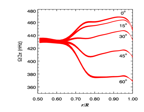
Figure 1: The internal solar rotation from helioseismology. The lines are marked by correspondent latitude values (courtesy NSF’s National Solar Observatory).

The given picture of the internal solar rotation suggests that some coupling must exist between the base of convection zone and the inner core. Otherwise, the rotational braking of the Sun on evolutionary time-scales would produce a rapidly rotating core (Dicke 1970). More than that, an even stronger link between low and high latitudes operates immediately below the base of convection zone in order to produce the rotation profile within the tachocline. The magnetic theory which explains the tachocline structure as a consequence of a weak internal fossil magnetic field simultaneously provides both the links (Rüdiger & Kitchatinov 1997; MacGregor & Charbonneau 1999). The present paper summarizes the basic ideas of the magnetic theory and describes new results of numerical MHD to model the tachocline and probing the internal field structure. Other approaches has been recently reviewed by Gilman (2005) and Garaud (2007).

Section 3 formulates the equations of the tachocline model and shows their solution for prescribed geometry of the fossil magnetic field within the radiative core. The role of meridional flow penetrating the uppermost region of the radiative core from the convection zone is discussed in section 4. In this section, the eigenmodes of internal poloidal field are computed with inclusion of the penetrating flow. Tachocline models with consistently defined internal field modes are discussed in section 5. In the final section 6 a first step is presented to understand the stability problem of the solar tachocline. In a hydrodynamical approach the 2D Watson theory for the stability of latitudinal differential rotation is reformulated in 3D with surprising results. The modes with small radial wavelengts are most unstable so that it is indeed essential for tachocline theories to take into account all the radial stratifications.

2 An heuristic approach

The basic parameters of the tachocline theory can be estimated as follows. The estimates are made with a simplified shear flow model in Cartesian geometry sketched in figure 2. The plane of $z=0$ mimics the bottom of the convection zone where a shear flow $\bi{u}=\left(U(y,z),0,0\right)$ imitating the differential rotation is prescribed as

$$U=U_{0}\sin\left(ky\right)\ \ \mathrm{at}\ z=0.$$ (1)

The Cartesian coordinates $x,y$ and $z$ correspond to azimuth, latitude and depth beneath the convection zone. An uniform (poloidal) field $\bi{B}_{0}$ along the $y$-axis is prescribed in the radiative zone. The shear flow penetrates the $z>0$ region and produces an $x$-component $B(y,z)$ of the field so that

$$\bi{B}=\left(B(y,z),B_{0},0\right).$$ (2)

can be written.

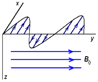
Figure 2: A shear flow is prescribed at $z=0$. Its penetration into the region of $z>0$ where the magnetic field $\bi{B}_{0}$ exists mimics the magnetic tachocline formation.

The equations for the stationary (toroidal) $x$-components of both magnetic and velocity fields then read

$$\nu\left(\frac{\partial^{2}U}{\partial y^{2}}+\frac{\partial^{2}U}{\partial z^{2}}\right)+\frac{B_{0}}{\mu_{0}\rho}\frac{\partial B}{\partial y}=0,\qquad\eta\left(\frac{\partial^{2}B}{\partial y^{2}}+\frac{\partial^{2}B}{\partial z^{2}}\right)+B_{0}\frac{\partial U}{\partial y}=0,$$ (3)

where $\nu$ is the viscosity and $\eta$ the magnetic diffusivity. The boundary condition for the flow is (1). For the toroidal field we impose the vacuum condition $B=0$ at $z=0$ motivated by the very large turbulent magnetic diffusivity inside the convection zone compared with microscopic diffusivity of the radiative interior. The remaining two conditions require $U$ and $B$ to vanish for $z\rightarrow\infty$.

The solution of the equations (3) simply reads

$$U(y,z) = U_{0}\exp\left(-\lambda_{1}kz\right)\cos\left(\lambda_{2}kz\right)\sin ky,$$

$$B(y,z) = \sqrt{\mu_{0}\rho}\ U_{0}\mathrm{Pm}^{1/2}\exp\left(-\lambda_{1}kz\right)\sin\left(\lambda_{2}kz\right)\cos ky,$$ (4)

where $\mathrm{Pm}=\nu/\eta$ is the magnetic Prandtl number and the parameters

$$\lambda_{1} = \left(1+\mathrm{Ha}^{2}\right)^{1/4}\cos\left({\textstyle\frac{1}{2}}\mathrm{arctanHa}\right),$$

$$\lambda_{2} = \left(1+\mathrm{Ha}^{2}\right)^{1/4}\sin\left({\textstyle\frac{1}{2}}\mathrm{arctanHa}\right)$$ (5)

depend on the Hartmann number

$$\mathrm{Ha}=\frac{B_{0}}{k\sqrt{\mu_{0}\rho\nu\eta}},$$ (6)

which is the basic parameter of the whole theory.

With Ha = 0, the equation (5) gives $\lambda_{1}=1$, $\lambda_{2}=0$, and (4) converts into the nonmagnetic solution, $B=0,\ U=U_{0}\rme^{-kz}\sin ky$. The resulting shear flow penetrates deep inside the $z>0$ region. No slender tachocline can be formed without magnetic fields. But with solar parameters one finds $\mathrm{Ha}\simeq 10^{7}B_{0}$ ($B_{0}$ in G) just below the convection zone. Very large Ha can thus be expected. For this case, $\lambda_{1}=\lambda_{2}=\sqrt{\mathrm{Ha}/2}$, and the solution (4) provides two important consequences:

(i) The tachocline thickness, $D_{\mathrm{tach}}$, is strongly reduced compared to its nonmagnetic value, $D_{0}$,

$$D_{\mathrm{tach}}=D_{0}\sqrt{\frac{2}{\mathrm{Ha}}}\simeq\sqrt{\frac{D_{0}}{B_{0}}}\left(\mu_{0}\rho\nu\eta\right)^{1/4}.$$ (7)

The tachocline is so thin because its extension in $z$-direction is only due to viscous stress while the smoothing in $y$-direction is performed by the much stronger Maxwell stress.

(ii) The amplitude of the toroidal magnetic field in the steady tachocline does not depend on the poloidal field strength, i.e.

$$B=U_{0}\sqrt{\mu_{0}\rho\ \mathrm{Pm}}.$$ (8)

The ratio of magnetic to kinetic energy in the tachocline equals Pm. In terms of the Alfvén velocity, $V_{\mathrm{A}}=B/\sqrt{\mu_{0}\rho}$, one finds

$$V_{\mathrm{A}}=\sqrt{\mathrm{Pm}}\ U_{0}$$ (9)

predicting $B\sim 1000$ G for the Sun.

After (7) even a weak poloidal field of only $B_{0}\sim 10^{-3}$ G can reduce $D_{\mathrm{tach}}$ below 5% of the solar radius. Equation (7) does also apply when $B_{0}$ is not an internal field of the radiative core. In case the poloidal field of the solar cycle diffuses into the core (Forgács-Dajka & Petrovay 2002) $\nu$ and $\eta$ must be replaced by the turbulent diffusivity values. As their magnetic Prandtl number is not much smaller than unity the resulting toroidal magnetic field after (9) becomes much stronger than 1000 G.

3 Tachocline model in spherical geometry

The tachocline equations will be formulated for axial symmetry. Then the magnetic field can be expressed in terms of $A$ and $B$ in accord to

$$\bi{B}={\mathbf{e}}_{\phi}B+\nabla\times\left({\mathbf{e}}_{\phi}\frac{A}{r\sin\theta}\right),$$ (10)

where $r,\theta$ and $\phi$ are spherical coordinates and $\mathbf{e}_{\phi}$ is the azimuthal unit vector. In the next section we show that meridional flow is only significant for the structure of the poloidal field. It can be neglected in the tachocline equations below. Here the only mean flow is the differential rotational with $\Omega=\Omega(r,\theta)$.

If the poloidal field is given, the tachocline is described by the equations for the toroidal field $B$ and the angular velocity $\Omega$

$$\frac{\eta}{r}\frac{\partial}{\partial\theta}\left(\frac{1}{\sin\theta}\frac{\partial\left(B\sin\theta\right)}{\partial\theta}\right)+\frac{\partial}{\partial r}\left(\eta\frac{\partial\left(Br\right)}{\partial r}\right)=\frac{\partial\Omega}{\partial\theta}\frac{\partial A}{\partial r}-\frac{\partial\Omega}{\partial r}\frac{\partial A}{\partial\theta},$$

$$\frac{\rho\nu}{\sin^{3}\theta}\frac{\partial}{\partial\theta}\left(\sin^{3}\theta\frac{\partial\Omega}{\partial\theta}\right)+\frac{1}{r^{2}}\frac{\partial}{\partial r}\left(r^{4}\rho\nu\frac{\partial\Omega}{\partial r}\right)=$$

$$\qquad=\frac{1}{\mu_{0}r^{2}\sin^{3}\theta}\left(r\frac{\partial A}{\partial r}\frac{\partial\left(B\sin\theta\right)}{\partial\theta}-\sin\theta\frac{\partial A}{\partial\theta}\frac{\partial\left(Br\right)}{\partial r}\right).$$ (11)

The rotation profile at the top boundary is produced by the convection zone for which the expression

$$\Omega=2.9\left(1-0.15\cos^{2}\theta\right)\ \mu\mathrm{rad\ s}^{-1}\quad\mathrm{at}\ \ r=R_{\mathrm{in}},$$ (12)

is used derived by Charbonneau et al(1999a). The remaining boundary conditions are the vacuum condition for toroidal field on the top and the conditions for the regularity of the fields for $r=0$:

$$B|_{r=R_{\mathrm{in}}}=B|_{r=0}=\left.\frac{\partial\Omega}{\partial\theta}\right|_{r=0}=0.$$ (13)

The used diffusivity profiles are shown in figure 3. We do not expect turbulence in the radiative core and apply, therefore, the microscopic magnetic diffusivity

$$\eta=10^{13}T^{-3/2}\ \mathrm{cm}^{2}\mathrm{s}^{-1},$$ (14)

and the viscosity

$$\nu=\nu_{\mathrm{micro}}+\nu_{\mathrm{rad}},$$

$$\nu_{\mathrm{micro}}=1.2\cdot 10^{-16}\frac{T^{5/2}}{\rho}\ \mathrm{cm}^{2}\mathrm{s}^{-1},\quad\nu_{\mathrm{rad}}=2.5\cdot 10^{-25}\frac{T^{4}}{\kappa\rho}\ \mathrm{cm}^{2}\mathrm{s}^{-1}$$ (15)

(cf. Kippenhahn & Weigert 1994) including molecular ($\nu_{\mathrm{micro}}$) and radiative ($\nu_{\mathrm{rad}}$) parts; $\kappa$ is opacity.

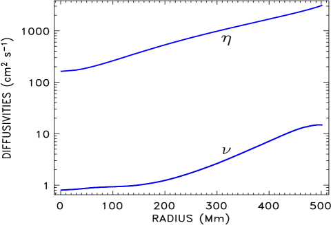
Figure 3: Radial profiles of magnetic diffusivity (14) and viscosity (15) calculated with the solar structure model by Stix & Skaley (1990).

The equations (11) with their boundary conditions (12), (13) provide tachocline solutions if the poloidal field is known. For a very first view the field model

$$A=B_{\mathrm{p}}\frac{r^{2}}{2}\left(1-\frac{r}{R_{\mathrm{in}}}\right)^{q}\sin^{2}\theta,\quad q>1$$ (16)

is used to probe whether slender tachoclines can indeed be found. $B_{\mathrm{p}}$ is the free amplitude of the poloidal field.

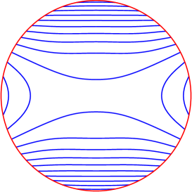
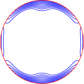
Figure 4: Isolines of the angular velocity of rotation inside the radiative core for the poloidal field model of (16) with $q=5$. The outer circle is the base of the convection zone. Left : $B_{\mathrm{p}}=0$. No tachocline exists. Right: $B_{\mathrm{p}}=0.01$ G. Tachocline exists.

Figure 4 compares the rotation pattern in a radiative zone computed with either zero magnetic field and with $B_{\mathrm{P}}=0.01$ G. $B_{\mathrm{P}}$ is the maximum strength of poloidal field inside the core. The maximum is attained in the core center. The field in the tachocline region is much weaker. Even this rather weak field suffices to produce a very strict and slender tachocline.

4 Magnetic field confinement by meridional flow

Our tachocline model is not yet consistent. It works with a prescribed poloidal field. We have shown that the model is not very sensitive to the poloidal field amplitude. Even a weak field can produce tachoclinic structures. The model is, however, very sensitive to the field geometry. The tachocline can be found only if the field lines are almost horizontal near the top of radiative zone. Steady rotation and magnetic fields can be realized in highly conducting fluids only with constant angular velocity along the field lines (Ferraro 1937). Therefore, the open field geometry with field lines crossing the boundary between convection and radiative zones is not appropriate for tachocline formation. The poloidal field prescribed by (16) is of a closed type. The field can, however, change to an open structure due to magnetic diffusion (Brun & Zahn 2006). We shall show in the following that already a small penetration of meridional flow from the convection zone into the radiative core produces the confined field geometry required for the tachocline formation (see Kitchatinov & Rüdiger 2006). If the electric conductivity in the core is high enough compared to that of the convection zone then the flow has massive consequences and the poloidal field lines in the transition zone become parallel to the meridional flow (cf. Mestel 1999).

4.1 Penetration of meridional circulation

A global poleward flow is observed at the solar surface (Komm et al1993) persisting to a depth of at least 12 Mm (Zhao & Kosovichev 2004). There must be a return flow towards the equator somewhere deeper. Theoretical models indeed predict an equatorward flow of $\sim 10$ m s^-1 at the base of convection zone (Kitchatinov & Rüdiger 1999; Miesch et al2000; Rempel 2005). This flow can penetrate beneath the bottom of the convection zone into the radiative core (figure 5). This penetration has been discussed recently in relation to dynamo models for solar activity (Nandy & Choudhuri 2002; Gilman & Miesch 2004; Rüdiger et al2005).

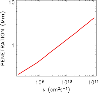
Figure 5: Left: Penetration depth as function of viscosity of the radiative core. Right: Meridional velocity in the penetration region at $45^{\circ}$ latitude for $\nu=1.1\cdot 10^{9}$ cm²s^-1. The vertical dotted line marks the bottom of the convection zone.

The penetration results from the viscous drag imposed by the meridional flow at the base of convection zone on the fluid beneath, and this is opposed by Coriolis force. The thickness of such an Ekman layer results as $D_{\mathrm{pen}}\sim\sqrt{\nu/\Omega}$ (see Gilman & Miesch 2004). The plot in the left of figure 5 is indeed approximated by $D_{\mathrm{pen}}\simeq 2.3\cdot\sqrt{\nu/\Omega}$ or, equivalently, by

$$D_{\mathrm{pen}}=1.4\cdot\sqrt{\nu}\cdot 10^{3}\ \mathrm{cm}$$ (17)

for solar parameters. The penetration distance is about 100 m for microscopic viscosity and remains shorter than 1 Mm for any reasonable value of eddy viscosity. The distance is small even compared to the tachocline depth, i.e. $D_{\mathrm{pen}}\ll D_{\mathrm{tach}}$.

This shallow penetration is, nevertheless, highly important for the geometry of the internal poloidal field. The ratio of the time $\tau_{\mathrm{diff}}=D^{2}_{\mathrm{pen}}/\eta$ for the magnetic field diffusion across the penetration layer to the characteristic time of induction of a meridional magnetic field from a radial one, $\tau_{\mathrm{s}}=D_{\mathrm{pen}}/u^{\mathrm{m}}$, gives the magnetic Reynolds number

$$\mathrm{Rm}=\frac{\tau_{\mathrm{diff}}}{\tau_{\mathrm{s}}}=\frac{D_{\mathrm{pen}}u^{\mathrm{m}}}{\eta}\simeq\frac{\mathrm{P}m}{\sqrt{\nu}}\cdot 10^{6}$$ (18)

(with $u^{\mathrm{m}}\simeq 10$ m s^-1 for the meridional velocity). This Reynolds number is large, Rm$\sim 10^{3}$, for microscopic diffusivities but it remains above this limit with eddy diffusivities up to $10^{6}$ cm²s^-1. The large ratio of (18) means that the latitudinal field inside the penetration layer is large compared to the radial field component. With other words, the field has just the confined geometry required for the tachocline formation. Only with eddy diffusivities of $10^{12}$ cm²s^-1 the Reynolds number (18) sinks to unity, so that only in this case the influence of penetration on the internal field geometry is too weak.

The ratio of $\tau_{\mathrm{diff}}$ to the advection time $\tau_{\mathrm{adv}}=R_{\mathrm{in}}/u^{\mathrm{m}}$

$$\frac{\tau_{\mathrm{diff}}}{\tau_{\mathrm{adv}}}=\frac{D_{\mathrm{pen}}}{R_{\mathrm{in}}}\ \mathrm{Rm}\simeq 0.03\ \mathrm{Pm}\ll 1,$$ (19)

is small independently of whether microscopic or eddy diffusivity is used. If the tachocline is stable in the hydrodynamic regime (see section 6) the microscopic diffusivities should be used. The small ratio (19) justifies the neglect of the meridional flow in the tachocline equations (11). The diffusion time, $\tau_{\mathrm{diff}}$, is too short as could the penetration layer be dynamo-relevant. The configuration of the internal poloidal field is probably the only process for which the penetration of the meridional circulation into the stable radiative zone is important.

4.2 A model of the poloidal field

For both axisymmetric flows and fields the poloidal magnetic field equation decouples from the tachocline equations (11) and reads

$$\frac{\partial A}{\partial t}=-\frac{u_{\theta}}{r}\frac{\partial A}{\partial\theta}-u_{r}\frac{\partial A}{\partial r}+\eta\frac{\partial^{2}A}{\partial r^{2}}+\frac{\eta}{r^{2}}\sin\theta\frac{\partial}{\partial\theta}\left(\frac{1}{\sin\theta}\frac{\partial A}{\partial\theta}\right),$$ (20)

where $\bi{u}$ is the velocity field. The vacuum boundary condition for the poloidal field can be applied on the top of the radiative zone because of the very large turbulent diffusivity in the convection zone,

$$\frac{\partial A}{\partial r}=\left(\frac{\partial A}{\partial r}\right)_{\mathrm{vac}}\quad{\rm at}\ \ \ r=R_{\mathrm{in}}.$$ (21)

The condition is usually formulated in terms of a Legendre polynomials expansion

$$A\left(r,\theta\right) = \sin\theta\sum\limits_{n=1}^{\infty}A_{n}\left(r\right)P_{n}^{1}\left(\cos\theta\right),$$

$$\left(\frac{\partial A}{\partial r}\right)_{\mathrm{vac}} = -\frac{\sin\theta}{r}\sum\limits_{n=1}^{\infty}nA_{n}\left(r\right)P_{n}^{1}\left(\cos\theta\right).$$ (22)

The other condition is $A=0$ at $r=0$.

The velocity $\bi{u}$ can be written with its stream function $\psi$ as

$$\bi{u}=\left(\frac{1}{\rho r^{2}\sin\theta}\frac{\partial\psi}{\partial\theta},-\frac{1}{\rho r\sin\theta}\frac{\partial\psi}{\partial r},r\sin\theta\ \Omega\right).$$ (23)

The meridional flow in the bulk of the radiative core is very slow. The characteristic time of the Eddington-Sweet circulation even exceeds the solar age (Tassoul 2000). Only the flow penetrating from convection zone is significant for the tachocline. The stream function, $\psi(r,\theta)$, of the penetrating flow drops to zero at a small depth of order $D_{\mathrm{pen}}$ inside the core. The function is, however, finite at the top boundary of the core where it scales as

$$\psi\left(R_{\mathrm{in}},\theta\right)=u^{\mathrm{m}}\rho R_{\mathrm{in}}D_{\mathrm{pen}}\hat{\psi}\left(\theta\right),$$ (24)

where $\hat{\psi}$ is dimensionless function of order unity. $u^{\mathrm{m}}$ is the meridional velocity amplitude at the boundary.

The penetration depth is so small even compared to tachocline thickness that we are motivated to integrate equation (20) across the penetration layer instead of resolving this layer explicitely. Such an integration reformulates the top boundary condition which now reads

$$R_{\mathrm{in}}\frac{\partial A}{\partial r}-\mathrm{Rm}\frac{\hat{\psi}\left(\theta\right)}{\sin\theta}\frac{\partial A}{\partial\theta}=R_{\mathrm{in}}\left(\frac{\partial A}{\partial r}\right)_{\mathrm{vac}},$$ (25)

where Rm is the magnetic Reynolds number (18) and the RHS is defined in (22). For $\rm Rm=0$ (25) reduces to the vacuum condition (21). The true Reynolds number is $\mathrm{Rm}\sim 10^{3}$.

Penetrating meridional flow is now included via the condition (25) and poloidal field structure can be found by solving eigenvalue problem for diffusion equation,

$$-\frac{A}{\tau}=\eta\frac{\partial^{2}A}{\partial r^{2}}+\frac{\eta}{r^{2}}\sin\theta\frac{\partial}{\partial\theta}\left(\frac{1}{\sin\theta}\frac{\partial A}{\partial\theta}\right),$$ (26)

where eigenvalue $\tau$ is the time of resistive decay of normal modes. The results discussed below were obtained in computations with the simplest stream function,

$$\hat{\psi}\left(\theta\right)=-\sin\theta\bar{P}^{1}_{2}\left(\cos\theta\right),$$ (27)

where $\bar{P}^{1}_{2}$ is the normalized Legendre polynomial.

The penetrating flow is expected to confine the internal poloidal field within the radiative core. The parameter

$$\delta\phi=\frac{\mathrm{max}|A\left(r,\theta\right)|_{r=R_{\mathrm{b}}}}{\mathrm{max}|A\left(r,\theta\right)|_{r\leq R_{\mathrm{b}}}},$$ (28)

is used to estimate the field confinement. The $\delta\phi$-parameter (28) estimates the ratio of the magnetic flux through the surface of the core to the characteristic value of the flux within the core.

The linear equations (26) and (25) define the field structure but not its amplitude. The amplitude $B_{\mathrm{p}}$ of the poloidal field is a free parameter of the model.

4.3 Normal modes of the internal field

How the structure of the internal field changes towards a confined geometry as Rm increases is shown in figure 6. The internal field computed with $\rm Rm=0$ has an open structure. Even a moderate flow with $\rm Rm=10$ changes the field considerably towards the confined geometry. The internal field for the solar value $\rm Rm=1000$ shown in figure 6 is almost totally confined. Less than 1% of magnetic flux belongs to ‘open’ field lines in this case (figure 7).

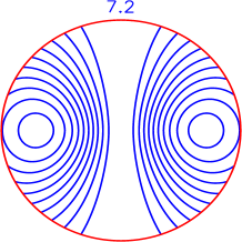
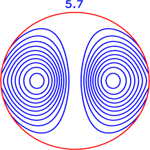
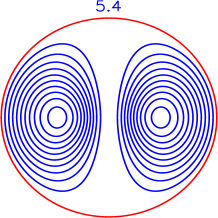
Figure 6: Field lines for the longest-living dipolar modes of poloidal field for different Rm. The Reynolds number varies as $\rm Rm=0,\ 10,\ 1000$ from left to right. The outer circle is the base of convection zone. The decay times in Gyr are marked at the tops.

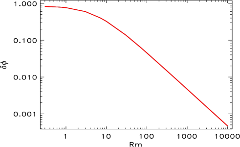
Figure 7: Confinement parameter (28) for the longest-living dipolar modes as function of the magnetic Reynolds number Rm.

The figures 6 and 7 only display the most slowly decaying dipolar modes. Other normal modes have shorter scales in radius or latitude and also shorter decay times. The three modes following the longest-living dipole ordered for decreasing lifetimes are shown in figure 8. The higher-order modes also have a confined structure. The decay times of the given normal modes are long enough to allow tachocline computations with steady poloidal fields.

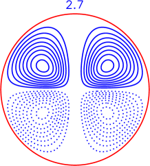
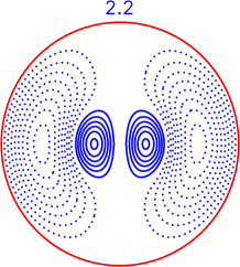
Figure 8: Normal modes of internal field following the dipolar mode of figure 6 for shorter lifetimes. The decay times (in Gyr) are shown on the top. The confinement parameter (28) varies as 0.0051, 0.0073, 0.0026 from left to right. $\rm Rm=1000$.

For sufficiently high Rm the direction of the penetrating meridional flow does not play a role. The flow from equator to poles also makes efficient confinements of the internal field. The effect can be understood as a magnetic field expulsion from the region of circulating motion (Weiss 1966). The transition from convection zone to radiative core was treated as a sharp boundary in our model. A smooth decrease of eddy diffusivity in convection zone towards its base may also contribute to the field confinement via the diamagnetic effect of inhomogeneous turbulence (cf. Krause & Rädler 1980).

5 Tachocline models

Figure 9 shows the angular velocity distributions inside the core computed with dipolar eigenmodes of internal field of various strengths. Dependence of the tachocline thickness on poloidal field amplitude is shown in figure 10 ($D_{\mathrm{tach}}$ was defined as depth of exponential decrease of equator-to-pole difference in angular velocity). Even a very weak field, $B_{\mathrm{p}}\sim 10^{-3}$ G, can produce tachocline. The depth $D_{\mathrm{tach}}$ drops below 5% of the solar radius for $B_{\mathrm{p}}>5\ \mathrm{mG}$.

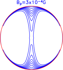
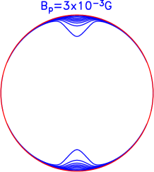
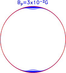
Figure 9: Angular velocity isolines in the radiative core computed with dipolar internal fields for $\rm{Rm}=1000$ for various poloidal field amplitudes (marked at the top).

The tachocline thickness in relation to the amplitude to the prescribed fossil field is given in figure 10. It is very close to the rough estimate (7). The simulations also confirm the above finding that the toroidal field amplitude, $B_{\mathrm{t}}=100...200$ G, hardly varies while the poloidal field amplitude changes by several orders of magnitude.

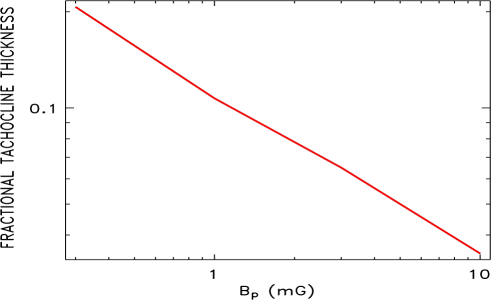
Figure 10: The fractional tachocline thickness as function of the amplitude, $B_{\mathrm{p}}$, of the internal poloidal field. Rm$=1000$.

Also the higher order modes given in figure 8 also produce tachoclinic structures provided that the fields have the confined structure which is always the case for Rm$=100$ or larger.

Figures 9 and 10 are valid for $\rm Rm=1000$. Already $\rm Rm=100$ suffices for tachocline formation, but for smaller Rm the poloidal field remains ‘too open’ for the formation of a tachocline. With other words, a meridional flow with minimum 1 m s^-1 amplitude at the base of convection zone is necessary for the success of the magnetic tachocline theory. The rather shallow penetration of the meridional flow of the convection zone into the radiative core influences the internal field geometry strongly enough and in such a way that the field becomes appropriate for the tachocline formation. We suggest that a layer thiner than 1 Mm beneath the convection zone where a meridional flow of 1-10 m s^-1 enters the radiative core is responsible for the existence of the solar tachocline.

6 Hydrodynamic stability: the Watson approach in 3D

Latitudinal differential rotation can be unstable even without magnetic field if the shear $\partial\Omega/\partial\theta$ is positive and sufficiently strong (Watson 1981). The critical value of 29% latitudinal shear found by Watson for the nonaxisymmetric mode with $m=1$ resulted from a theory with strong stratification but without any radial velocity and radial wavelengths. The value has also appeared in a 3D numerical examination of marginal stability of a shell rotating fast enough with the rotation law

$$\Omega=\Omega_{0}\left(1-a\cos^{2}\theta\right),$$ (29)

but of fully incompressible material (Arlt et al2007). The critical shear increases to higher values, however, if the real rotation law (including its radial variations) of the solar tachocline is adopted. In this case the superrotation observed in the equatorial region of the rotation law strongly stabilizes the shear instability.

In this section the Watson approach with strong density stratification (for $m=1$) is extended to 3D, i.e. to the inclusion of finite radial velocities and finite radial wavelengths. The stabilizing effect of a subadiabatic stratification on the mean flow is characterized by the buoyancy frequency,

$$N^{2}=\frac{g}{C_{\mathrm{p}}}\frac{\partial S}{\partial r},$$ (30)

where $S=C_{\mathrm{v}}\ln\left(P/\rho^{\gamma}\right)$ is the specific entropy of ideal gas. The frequency is very large in the solar radiative core (see figure 11).

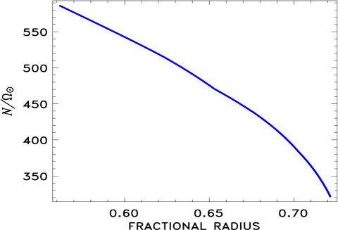
Figure 11: The buoyancy frequency (30) in the upper radiative core after the solar model of Stix & Skaley (1990).

The larger the $N$ the more the radial fluctuations are suppressed by the buoyancy force. Radial velocities should therefore be small. Our stability analysis is local in the radial dimension, i.e. we use Fourier modes $\exp{\mathrm{i}kr}$ with $kr\gg 1$. The equation system remains, however, global in horizontal dimensions.

Instabilities of rotating shear flows are fast. Their growth rates are of order $\Omega$ or smaller. In the short-wave approximation the velocity field can be assumed as divergence-free, $\mathrm{div}{\bi u}^{\prime}=0$. The next assumption concerns the pressure. Local thermal disturbances occur at constant pressure so that $\rho^{\prime}/\rho=-T^{\prime}/T$ or $S^{\prime}=-C_{\mathrm{p}}\rho^{\prime}/\rho$ where perturbations have been marked by dashes. This assumption is again justified by the incompressible nature of the fluid. We start from the linearized equations of velocity, i.e.

$$\frac{\partial{\bi u}^{\prime}}{\partial t}+\left({\bi u}\cdot\nabla\right){\bi u}^{\prime}+\left({\bi u}^{\prime}\cdot\nabla\right){\bi u}=-\left(\frac{1}{\rho}\nabla p\right)^{\prime}+\nu\Delta{\bi u}^{\prime}$$ (31)

and entropy

$$\frac{\partial S^{\prime}}{\partial t}+{\bi u}\cdot\nabla S^{\prime}+{\bi u}^{\prime}\cdot\nabla S=\frac{C_{\mathrm{p}}\chi}{T}\Delta T^{\prime}.$$ (32)

The basic flow is the rotation law (29).

Perturbations of velocity and pressure are now expressed in terms of scalar potentials like

$${\bi u}^{\prime}=\frac{{\bi e}_{r}}{r^{2}}\hat{L}P-\frac{{\bi e}_{\theta}}{r}\left(\frac{1}{\sin\theta}\frac{\partial T}{\partial\phi}+\frac{\partial^{2}P}{\partial r\partial\theta}\right)+\frac{{\bi e}_{\phi}}{r}\left(\frac{\partial T}{\partial\theta}-\frac{1}{\sin\theta}\frac{\partial^{2}P}{\partial r\partial\phi}\right),$$ (33)

with the operator

$$\hat{L}=\frac{1}{\sin\theta}\frac{\partial}{\partial\theta}\sin\theta\frac{\partial}{\partial\theta}+\frac{1}{\sin^{2}\theta}\frac{\partial^{2}}{\partial\phi^{2}}.$$ (34)

The identities

$$r\left({\bi r}\cdot\nabla\times{\bi u}^{\prime}\right) = \hat{L}T,\ \ \ r^{3}\left({\bi r}\cdot\nabla\times\nabla\times{\bi u}^{\prime}\right)=\left(\hat{L}+r^{2}\frac{\partial^{2}}{\partial r}\right)\hat{L}P,$$ (35)

are used to reformulate the relations in terms of the potentials.

The perturbations are considered as Fourier modes for time, azimuth and radius in the form $\mathrm{exp}\left(\mathrm{i}(-\omega t+m\phi+kr)\right)$. For an instability the eigenvalue $\omega$ must possess a positive imaginary part. Only the highest order terms in $kr$ for the same variable have been considered. The pressure term in (31) can be formulated as

$${\bi r}\cdot\nabla\times\nabla\times\left(\frac{1}{\rho}\nabla p\right)^{\prime} = -{\bi r}\cdot\nabla\times\left(\frac{1}{\rho^{2}}(\nabla\rho)\times(\nabla p)\right)^{\prime}=$$

$$\frac{\bi r}{C_{\mathrm{p}}}\cdot\nabla\times\left(\frac{1}{\rho}(\nabla S)\times(\nabla p)\right)^{\prime} = -\frac{\bi r}{C_{\mathrm{p}}}\cdot\nabla\times\left({\bi g}\times\nabla S^{\prime}\right)=\frac{g}{rC_{\mathrm{p}}}\hat{L}S^{\prime}.$$ (36)

In order to denormalize the variables time is measured in units of $\Omega_{0}^{-1}$ and velocities are scaled with $r\Omega_{0}$. The remaining variables are

$$V=\frac{k}{\Omega_{0}r^{2}}\ P,\ \ W=\frac{1}{\Omega_{0}r^{2}}\ T,\ \ s=\frac{\mathrm{i}krg}{C_{\mathrm{p}}rN^{2}}\ S^{\prime},\ \ \ \ \hat{\Omega}=\frac{\Omega}{\Omega_{0}}.$$ (37)

Then the equation for the poloidal flow reads

$$\hat{\omega}\left(\hat{L}V\right) = -\hat{\lambda}^{2}\left(\hat{L}s\right)-\mathrm{i}\frac{\epsilon_{\nu}}{\hat{\lambda}^{2}}\left(\hat{L}V\right)-$$ (38)

$$- 2\mu\hat{\Omega}\left(\hat{L}W\right)-2\left(1-\mu^{2}\right)\frac{\partial\left(\mu\hat{\Omega}\right)}{\partial\mu}\frac{\partial W}{\partial\mu}-2m^{2}\frac{\partial\hat{\Omega}}{\partial\mu}W+$$

$$+ m\hat{\Omega}\left(\hat{L}V\right)+2m\frac{\partial\left(\mu\hat{\Omega}\right)}{\partial\mu}V+2m\left(1-\mu^{2}\right)\frac{\partial\hat{\Omega}}{\partial\mu}\frac{\partial V}{\partial\mu},$$

with $\mu=\cos\theta$ and the normalized radial wavelength

$$\hat{\lambda}=\frac{N}{\Omega_{0}kr}.$$ (39)

The first term on the RHS describes the stabilizing effect of the stratification. It vanishes for small $\hat{\lambda}$. Apart from this stabilizing buoyancy term, the wavelength only exists in diffusive terms. The second term of the RHS includes the action of viscosity. Here we have used the quantities

$$\epsilon_{\nu}=\frac{\nu N^{2}}{\Omega_{0}^{3}r^{2}},\ \ \ \ \ \ \ \ \ \ \ \ \ \epsilon_{\chi}=\frac{\chi N^{2}}{\Omega_{0}^{3}r^{2}}$$ (40)

for the diffusive parameters $\nu$ and $\chi$. Now the limit $N\to 0$ can no longer be used for the transition to nonstratified but viscous media. The numerical values for the solar tachocline are

$$\epsilon_{\nu}=2\cdot 10^{-10},\ \ \ \ \ \ \ \ \ \ \ \ \ \epsilon_{\chi}=10^{-4}.$$ (41)

The second and the following lines in (38) describe the influences of the basic rotation. Note that only latitudinal derivatives of $\Omega$ appear.

The complete system of equations also includes the equation for toroidal flow,

$$\hat{\omega}\left(\hat{L}W\right)=-\mathrm{i}\frac{\epsilon_{\nu}}{\hat{\lambda}^{2}}\left(\hat{L}W\right)+m\hat{\Omega}\left(\hat{L}W\right)-mW\frac{\partial^{2}}{\partial\mu^{2}}\left(\left(1-\mu^{2}\right)\hat{\Omega}\right)+$$

$$+\left(\hat{L}V\right)\frac{\partial}{\partial\mu}\left(\left(1-\mu^{2}\right)\hat{\Omega}\right)+\left(\frac{\partial}{\partial\mu}\left(\left(1-\mu^{2}\right)^{2}\frac{\partial\hat{\Omega}}{\partial\mu}\right)-2\left(1-\mu^{2}\right)\hat{\Omega}\right)\frac{\partial V}{\partial\mu},$$ (42)

and the entropy equation

$$\hat{\omega}s=-\mathrm{i}\frac{\epsilon_{\chi}}{\hat{\lambda}^{2}}s+m\hat{\Omega}s+\hat{L}V.$$ (43)

Note that for the Reynolds number ${\rm Re}=\Omega r^{2}/\nu$ follows

$${\rm Re}=\frac{N^{2}/\Omega^{2}}{\epsilon_{\nu}},$$ (44)

which with (41) is very large.

For positive $a$ in (29) the modes A1 and S2 become unstable for sufficiently large $a=a_{\rm crit}$. Figure 12 shows the dependence of the $a_{\rm crit}$ on the normalized wavelength $\hat{\lambda}$. Of course, for large enough radial wavelength the 29%-value of the Watson theory with 2D fluctuations is reproduced. It is reduced, however, to $a=0.21$ in the full 3D model calculations. We see that in contrast to the original Watson approach short rather than long radial scales are preferred. The minimum $a_{\rm crit}$ appears for $\hat{\lambda}\simeq 0.6$, so that the characteristic wavelength of $\lambda\simeq 6$ Mm results for the solar tachocline. For shorter scales the instability for $m=1$ disappears due to the action of the dissipation processes but modes with higher $m$ remain still unstable.

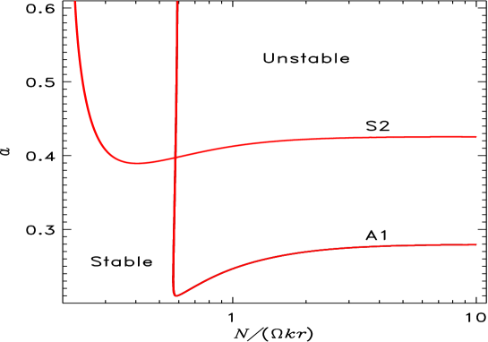
Figure 12: Stability map for latitudinal differential rotation (3D hydrodynamics). Most unstable are the perturbation modes with the vertical scale $\hat{\lambda}\simeq 0.6$. The critical magnitude of latitudinal shear is reduced to 0.21 compared to the 0.29 value for large wavelengths. For short wavelengths the instability for $m=1$ rapidly disappears by dissipation effects.

7 Concluding remarks

The presence of a meridional flow with an amplitude of a few meters per second at the bottom of the convection zone is shown as necessary for the magnetic tachocline model. The flow provides the confined geometry (with field lines parallel to the outer spherical boundary) of the internal magnetic field which is necessary for the tachocline formation. The bottom flow is also a key ingredient of advection-dominated dynamo models for the solar cycle (see Rüdiger & Hollerbach 2004 for detailed references). The flow was predicted theoretically but its existence is not yet confirmed by observations. We hope, of course, that helioseismology will probe the deep meridional flow soon.

The polar cusps in the tachoclines of figure 9 are consequences of the assumed axisymmetry. This assumption may not be realistic. The penetrating meridional flow is, however, expected to confine even nonaxisymmetric fields to the core so that the fields should also be able to produce the tachoclinic structures.

The tachocline computations result in toroidal fields of 100 to 200 G, much stronger than the original poloidal fields. These toroidal fields can be subject to current-driven pinch-type instabilities (Tayler 1973). Hence, the question is whether the steady axisymmetric solutions of our model are stable against all the nonaxisymmetric disturbances. The threshold field strength for the instability were estimated to be of order $10^{2\dots 3}$ G (Spruit 1999; Arlt et al2007; Kitchatinov & Rüdiger 2007) what is (only) somewhat larger than the field amplitudes in our model.

It is important for the magnetic tachocline model that the magnetic Reynolds number (18) is large. This is true for microscopic diffusivity or for not too large eddy diffusivities up to about 10⁸ cm²s^-1. The tachocline should, therefore, be stable or only mildly turbulent to allow poloidal field confinement by meridional flow. Some low level of turbulence may, however, be even necessary. The magnetic field is so efficient in producing tachocline structures that poloidal fields of only 1 G lead to radial scales smaller than 1% of the solar radius. It is, however, $D_{\mathrm{tach}}\simeq 0.04R_{\odot}$. Hence, the internal poloidal field must be (much) smaller than 1 G (Kitchatinov et al2001) or, if it is not, some kind of instability may prevent the tachocline thickness to reduce below the helioseismologically detected level.

The stability issue is a clear perspective for future tachocline studies. As a corresponding application we have developed in the last section the 2D theory of Watson (1981) for the hydrodynamic instability of latitudinal differential rotation to a fully 3D theory. Now the critical wavelength of the unstable mode with $m=1$ is only 6 Mm while the critical latitudinal shear (see (29)) is reduced from 29% to 21%. This (linear) theory works with a Prandtl number of order $10^{-6}$ and a very high Reynolds number of order $10^{12}$.

References

References

- [1] [] Antia H M, Basu S and Chitre S M 1998 Mon. Not. Roy. Astron. Soc. 298 543
- [2] [] Arlt R, Sule A and Rüdiger G 2007 Astron. Astrophys. 461 295
- [3] [] Basu S and Antia H M 1997 Mon. Not. Roy. Astron. Soc. 287 189
- [4] [] Brun A S and Zahn J-P 2006 Astron. Astrophys. 457 665
- [5] [] Charbonneau P, Dikpati M and Gilman P A 1999a Astrophys. J. 526 523
- [6] [] Charbonneau P, Christensen-Dalsgaard J, Henning R, Larsen R M, Schou J, Thompson M J and Tomczyk S 1999b Astrophys. J. 527 445
- [7] [] Christensen-Dalsgaard J, Gough D O and Thompson M J 1991 Astrophys. J. 287 189
- [8] [] Dicke R H 1970 Ann. Rev. Astron. Astrophys. 8 297
- [9] [] Ferraro V C A 1937 Mon. Not. Roy. Astron. Soc. 97 458
- [10] [] Forgács-Dajka E and Petrovay K 2002 Astron. Astrophys. 389 629
- [11] [] Garaud P 2007 Dynamics of the Solar Tachocline, Chapter 8 in The Solar Tachocline. Eds. D W Hughes, R Rosner and N O Weiss (Cambridge: Cambridge Univ. Press) to appear
- [12] [] Gilman P A 2005 Astron. Nachr. 326 208
- [13] [] Gilman P A and Miesch M S 2004 Astrophys. J. 611 568
- [14] [] Kippenhahn R and Weigert A 1994 Stellar Structure and Evolution (Berlin Heidelberg New York: Springer-Verlag)
- [15] [] Kitchatinov L L and Rüdiger G 1999 Astron. Astrophys. 344 911
- [16] [] Kitchatinov L L, Jardine M and Cameron A C 2001 Astron. Astrophys. 374 250
- [17] [] Kitchatinov L L and Rüdiger G 2006 Astron. Astrophys. 453 329
- [18]
- [19] [] Kitchatinov L L and Rüdiger G 2007 Astron. Astrophys.
- [20] [] Komm R W, Howard R F and Harvey J W 1993 Sol. Phys. 147 207
- [21] [] Kosovichev A G 1996 Astrophys. J. 469 L61
- [22] [] Kosovichev A G et al1997 Sol. Phys. 170 43
- [23]
- [24] [] Krause F and Rädler K H 1980 Mean-Field Magnetohydrodynamics and Dynamo Theory (Oxford: Pergamon Press)
- [25]
- [26] [] MacGregor K B and Charbonneau P 1999 Astrophys. J. 519 911
- [27] [] Mestel L 1999 Stellar Magnetism (Oxford: Clarendon Press)
- [28] [] Miesch M S, Elliott J R, Toomre J et al2000 Astrophys. J. 532 593
- [29] [] Nandy D and Choudhuri A R 2002 Science 296 1671
- [30] [] Rempel M 2005 Astrophys. J. 622 1320
- [31] [] Rüdiger G and Kitchatinov L L 1997 Astron. Nachr. 318 273
- [32] [] Rüdiger G and Hollerbach R L 2004 The Magnetic Universe (Berlin: Wiley-VCH)
- [33] [] Rüdiger G, Kitchatinov L L and Arlt R 2005 Astron. Astrophys. 444 L53
- [34] [] Schou J et al1998 Astrophys. J. 505 390
- [35] [] Spruit H C 1999 Astron. Astrophys. 349 189
- [36] [] Stix M and Skaley D 1990 Astron. Astrophys. 232 234
- [37] [] Tassoul J-L 2000 Stellar Rotation (Cambridge: Cambridge University Press)
- [38] [] Tayler R J 1973 Mon. Not. Roy. Astron. Soc. 161 365
- [39] [] Watson M 1981 Geophys. Astrophys. Fluid Dyn. 16 285
- [40] [] Weiss N O 1966 Proc. Roy. Soc. London A 293 310
- [41] [] Wilson P R, Burtonclay D and Li Y 1997 Astrophys. J. 489 395
- [42] [] Zhao J and Kosovichev A G 2004 Astrophys. J. 603 776