A unifying framework for self-consistent gravitational lensing
and stellar dynamics analyses of early-type galaxies

Abstract

Gravitational lensing and stellar dynamics are two independent methods, based solely on gravity, to study the mass distributions of galaxies. Both methods suffer from degeneracies, however, that are difficult to break. In this paper, we present a new framework that self-consistently unifies gravitational lensing and stellar dynamics, breaking some classical degeneracies that have limited their individual usage, particularly in the study of high-redshift galaxies.

For any given galaxy potential, the mapping of both the unknown lensed source brightness distribution and the stellar phase-space distribution function onto the photometric and kinematic observables can be cast as a single set of coupled linear equations, which are solved by maximizing the likelihood penalty function. The Bayesian evidence penalty function subsequently allows one to find the best potential-model parameters and to quantitatively rank potential-model families or other model assumptions (e.g. PSF). We have implemented a fast algorithm that solves for the maximum-likelihood pixelized lensed source brightness distribution and the two-integral stellar phase-space distribution function $f(E,L_{z})$, assuming axisymmetric potentials. To make the method practical, we have devised a new Monte Carlo approach to Schwarzschild’s orbital superposition method, based on the superposition of two-integral ($E$ and $L_{z}$) toroidal components, to find the maximum-likelihood two-integral distribution function in a matter of seconds in any axisymmetric potential. The non linear parameters of the potential are subsequently found through a hybrid MCMC and Simplex optimization of the evidence. Illustrated by the power-law potential models of Evans, we show that the inclusion of stellar kinematic constraints allows the correct linear and non linear model parameters to be recovered, including the potential strength, oblateness and inclination, which, in the case of gravitational-lensing constraints only, would otherwise be fully degenerate.

1. Introduction

Understanding the formation and the evolution of early-type galaxies is one of the most important open problems in present-day astrophysics and cosmology. Within the standard $\Lambda$CDM paradigm, massive ellipticals are predicted to be formed via hierarchical merging of lower mass galaxies (Toomre, 1977; Frenk et al., 1988; White & Frenk, 1991; Barnes, 1992; Cole et al., 2000). Despite the many theoretical and observational successes of this scenario, several important features of early-type galaxies are still left unexplained. In particular, the origin of the (often strikingly tight) empirical scaling laws that correlate the global properties of ellipticals remain unexplained: (i) the fundamental plane (Djorgovski & Davis, 1987; Dressler et al., 1987), relating effective radius, velocity dispersion and effective surface brightness; (ii) the $M_{\rm BH}-\sigma$ (Magorrian et al., 1998; Ferrarese & Merritt, 2000; Gebhardt et al., 2000), relating the mass of the central supermassive black hole hosted by the galaxy with its velocity dispersion; (iii) the color-$\sigma$ (Bower, Lucey, & Ellis, 1992) and the ${\rm Mg}_{2}-\sigma$ (Guzman et al., 1992; Bender, Burstein, & Faber, 1993; Bernardi et al., 2003) relating the velocity dispersion with the stellar ages and the chemical composition of the galaxy.

Each of these scaling relations relate structural, (spectro-) photometric, and dynamical (i.e. stellar velocity dispersion) quantities. Whereas the first two are solely based on the observed stellar component, the latter is a function of the stellar and dark matter mass distribution. Hence, a detailed study of the inner mass profile of early-type galaxies at different redshifts is undoubtedly necessary to properly address the numerous issues related with the formation and the evolution of these objects and their scaling relations, and it would also constitute an excellent test bed for the validity of the $\Lambda$CDM scenario on small (i.e. non linear) scales.

Today, a large number of thorough stellar dynamic and X-ray studies have been conducted to probe the mass structure of nearby ($z\lesssim 0.1$) early-type galaxies (Fabbiano, 1989; Mould et al., 1990; Saglia, Bertin, & Stiavelli, 1992; Bertin et al., 1994; Frank, van Gorkom, & de Zeeuw, 1994; Carollo et al., 1995; Arnaboldi et al., 1996; Rix et al., 1997; Matsushita et al., 1998; Loewenstein & White, 1999; Gerhard et al., 2001; Seljak, 2002; de Zeeuw et al., 2002; Borriello, Salucci, & Danese, 2003; Romanowsky et al., 2003; Cappellari et al., 2006; Gavazzi et al., 2007), in most (but not all) cases finding evidence for the presence of a dark matter halo component and for a flat equivalent rotation curve in the inner regions.

When it comes to distant ($z\gtrsim 0.1$) early-type galaxies, however, only relatively little is known. The two main diagnostic tools which can be employed to carry out such studies, namely gravitational lensing (Schneider et al., 2006) and stellar dynamics (Binney & Tremaine, 1987), both suffer from limitations and degeneracies. Gravitational lensing provides an accurate and almost model independent determination of the total mass projected within the Einstein radius, but a reliable determination of the mass density profile is often prevented by the effects of the mass sheet (Falco, Gorenstein, & Shapiro, 1985) and the related mass profile and shape degeneracies (e.g. Wucknitz, 2002; Evans & Witt, 2003; Saha & Williams, 2006). Despite these limitations, strong gravitational lensing has provided the first, although heterogeneous, constraints on the internal mass distribution of stellar and dark matter in high-redshift galaxies (e.g. Kochanek, 1995; Rusin & Ma, 2001; Ma, 2003; Rusin et al., 2002; Cohn et al., 2001; Muñoz et al., 2001; Winn et al., 2003; Wucknitz et al., 2004; Ferreras et al., 2005; Wayth et al., 2005; Dye & Warren, 2005; Brewer & Lewis, 2006b; Dobke & King, 2006).

Analyses based on stellar dynamics are limited by the paucity of bright kinematic tracers in the outer regions of early-type galaxies (e.g. Gerhard, 2006). Moreover, there is a severe degeneracy (the mass-anisotropy degeneracy) between the mass profile of the galaxy and the anisotropy of its stellar velocity dispersion tensor (e.g. Gerhard, 1993). Higher order velocity moments, which could be used to overcome this difficulty, cannot be measured in reasonable integration time for such distant systems with any of the current instruments.

A viable solution to break these degeneracies to a large extent is a joint analysis which combines constraints from both gravitational lensing and stellar dynamics (Koopmans & Treu, 2002; Treu & Koopmans, 2002, 2003; Koopmans & Treu, 2003; Rusin et al., 2003; Treu & Koopmans, 2004; Rusin & Kochanek, 2005; Bolton et al., 2006; Treu et al., 2006; Koopmans et al., 2006; Gavazzi et al., 2007): the two approaches can be described as almost “orthogonal”, in other words they complement each other very effectively (see e.g. Koopmans, 2004, for some simple scaling relations), allowing a trustworthy determination of the mass density profile of the lens galaxy in the inner regions (i.e. within the Einstein radius or the effective radius, whichever is larger). A joint gravitational lensing and stellar dynamics study of the Lenses Structure and Dynamics (LSD) and Sloan Lens ACS (SLACS) samples of early-type galaxies (Koopmans et al., 2006; Bolton et al., 2006; Treu et al., 2006), for example, showed that the total mass density has an average logarithmic slope extremely close to isothermal ($\langle s^{\prime}\rangle=2.01\pm 0.03$, assuming $\rho_{\rm tot}\propto r^{-s^{\prime}}$) with a very small intrinsic spread of at most 6%. They also find no evidence for any secular evolution of the inner density slope of early-type galaxies between $z=0.08$ and $1.01$ (Koopmans et al., 2006).

These authors, in their combined analysis, make use of both gravitational lensing and stellar dynamics information, but treat the two problems as independent. More specifically, the projected mass distribution of the lens galaxy is modeled as a singular isothermal ellipsoid (SIE; e.g. Kormann et al., 1994), and the obtained value for the total mass within the Einstein radius is used as a constraint for the dynamical modeling; in the latter the galaxy is assumed to be spherical and the stellar orbit anisotropy to be constant (or follow an Osipkov–Merritt profile; Osipkov, 1979; Merritt, 1985a, b) in the inner regions and therefore the spherical Jeans equations can be solved in order to determine the slope $s^{\prime}$ (see Koopmans & Treu, 2003; Treu & Koopmans, 2004; Koopmans et al., 2006, for a full discussion of the methodology). This approach, however, while being robust and successful, is not fully self-consistent: gravitational lensing and the stellar dynamics use different assumptions about the symmetry of the system and different potentials for the lens galaxy.

This has motivated us to develop a completely rigorous and self-consistent framework to carry out combined gravitational lensing and stellar dynamics studies of early-type galaxies, the topic of the present paper. The methodology that we introduce, in principle, is completely general and allows – given a set of data from gravitational lensing (i.e. the surface brightness distribution of the lensed images) and stellar dynamics (i.e. the surface brightness distribution and the line-of-sight projected velocity moments of the lens galaxy) – the “best” parameters, describing the gravitational potential of the galaxy and its stellar phase-space distribution function, to be recovered.

In practice, because of technical and computational limitations, we restrict ourselves to axisymmetric potentials and two-integral stellar phase-space distribution functions (i.e. $f(E,L_{z})$; see Binney & Tremaine, 1987), in order to present a fast and efficiently working algorithm. We introduce a new Monte Carlo approach to Schwarzschild’s orbital superposition method, that allows the $f(E,L_{z})$ to be solved in axisymmetric potentials in a matter of seconds. All of these restrictions, however, should be seen just as one particular implementation of the much broader general framework.

The very core of the methodology lies in the possibility of formulating both the lensed image reconstruction and the dynamical modeling as formally analogous linear problems. The whole framework is coherently integrated in the context of Bayesian statistics, which provides an objective and unambiguous criterion for model comparison, based on the evidence merit function (MacKay, 1992; Mackay, 2003). The Bayesian evidence penalty function allows one to both determine the “best” (i.e. the most plausible in an Occam’s razor sense) set of non linear parameters for an assigned potential and compare and rank different potential families, as well as set the optimal regularization level in solving the linear equations and find the best point-spread function (PSF) model, pixel scales, etc.

The paper is organized as follows: In Sect. 2 we first review some relevant aspects of the theory of Bayesian inference, and we elucidate how these apply to the framework of combined lensing and stellar dynamics. In Sect. 3 we present a general overview of the framework, with particular focus on the case of our implementation for axisymmetric potentials. In Sects. 4 and 5, respectively, we provide a detailed description of the methods for the lensed image reconstruction and the dynamical modeling. In Sect. 6 we describe the testing of the method, showing that it allows a reliable recovery of the correct model potential parameters. Finally, conclusions are drawn in Sect. 7. The application of the algorithm to the early-type lens galaxies of the SLACS sample (e.g. Bolton et al., 2006; Treu et al., 2006; Koopmans et al., 2006; Gavazzi et al., 2007) will be presented in forthcoming papers.

2. Data fitting and model comparison:
A Bayesian approach

Before describing the code itself in more detail, in this Section we first review the basics of Bayesian statistics. This is relevant, because – as will be shown in more detail in the coming Sections – both the lensing and stellar dynamics parts of the algorithm can be formalized as linear sets of equations

$$\vec{b}=\mathbf{A}\vec{x}+\vec{n}$$ (1)

that can be solved within a Bayesian statistical framework. In the above equation, $\vec{b}$ represents the data, $\mathbf{A}=\mathbf{A}[\Phi(\vec{\eta})]$ is the model, which will in general depend on the physics involved (e.g., in our case, the lens-galaxy potential $\Phi$, a function of the non linear parameters $\vec{\eta}$), $\vec{x}$ are the linear parameters that we want to infer, and $\vec{n}$ is the noise in the data, characterized by the covariance matrix $\mathbf{C}$.

First, we aim to determine the linear parameters $\vec{x}$ given the data and a fixed model and, on a more general level, to find the non linear parameters $\vec{\eta}$ corresponding to the “best” model. Note that the choices of grid size, PSF, etc., are also regarded as being (discrete) parameters of the model family (changing these quantities or assumptions formally is equivalent to adopting a different family of models).

Both of these problems can quantitatively be addressed within the framework of Bayesian statistics. Following the approach of MacKay (MacKay 1992, 1999, Mackay 2003; see also Suyu et al. 2006), it is possible to distinguish between three different levels of inference for the data modeling.

1. At the first level of inference, the model $\mathbf{A}$ is assumed to be true, and the most probable $\vec{x}_{\rm MP}$ for the linear parameters is obtained by maximizing the posterior probability, given by the expression (derived from Bayes’ rule)

   $$P(\vec{x}|\vec{b},\lambda,\mathbf{A},\mathbf{H})=\frac{P(\vec{b}|\vec{x},\mathbf{A})P(\vec{x}|\mathbf{H},\lambda)}{P(\vec{b}|\lambda,\mathbf{A},\mathbf{H})},$$ (2)

   where $\mathbf{H}$ is a regularization operator, which formalizes a conscious a priori assumption about the degree of smoothness that we expect to find in the solution (refer to Appendix A for the construction of the regularization matrix); the level of regularization is set by the hyperparameter value $\lambda$. The introduction of some kind of prior (the term $P(\vec{x}|\mathbf{H},\lambda)$ in Eq. [2]) is inescapable, since, due to the presence of noise in the data, the problem from equation (1) is an ill-conditioned linear system and, therefore, cannot simply be solved through a direct inversion along the line of $\vec{x}=\mathbf{A}^{-1}\vec{b}$ (see for example Press et al. 1992 for a clear introductory treatment on this subject). Note that besides $\mathbf{H}$, any a priori assumption (PSF, pixel scales, etc.) can be treated and ranked through the evidence. Traditional likelihood methods do not allow a proper quantitative ranking of model families or other assumptions. In Eq. (2), the probability $P(\vec{b}|\vec{x},\mathbf{A})$ is the likelihood term, while the normalization constant $P(\vec{b}|\lambda,\mathbf{A},\mathbf{H})$ is called the evidence and plays a fundamental role in Bayesian analysis, because it represents the likelihood term at the higher levels of inference.

2. At the second level, we infer the most probable hyperparameter $\lambda_{\rm MP}$ for the model $\mathbf{A}$ by maximizing the posterior probability function

   $$P(\lambda|\vec{b},\mathbf{A},\mathbf{H})=\frac{P(\vec{b}|\lambda,\mathbf{A},\mathbf{H})P(\lambda)}{P(\vec{b}|\mathbf{A},\mathbf{H})},$$ (3)

   which is equivalent to maximizing the likelihood $P(\vec{b}|\lambda,\mathbf{A},\mathbf{H})$ (i.e. the evidence of the previous level) if the prior $P(\lambda)$ is taken to be flat in logarithm, as is customarily done,, because its scale is not known.

3. Finally, at the third level of inference the models are objectively compared and ranked on the basis of the evidence (of the previous level),

   $$P(\mathbf{A},\mathbf{H}|\vec{b})\propto P(\vec{b}|\mathbf{A},\mathbf{H})P(\mathbf{A},\mathbf{H}),$$ (4)

   where the prior $P(\mathbf{A},\mathbf{H})$ is assumed to be flat. It has been shown by MacKay (1992) that this evidence-based Bayesian method for model comparison automatically embodies the principle of Occam’s razor, i.e. it penalizes those models which correctly predict the data, but are unnecessarily complex. Hence, it is in some sense analogous to the reduced $\chi^{2}$.

In Sections 2.1 and 2.2 we illustrate how this general framework is implemented under reasonable simplifying assumptions and how the maximization of the evidence is done in practice.

2.1. Maximizing the posterior: Linear optimization

If the noise $\vec{n}$ in the data can be modeled as Gaussian, it is possible to show (MacKay, 1992; Suyu et al., 2006) that the posterior probability (Eq. [2]) can be written as

$$P(\vec{x}|\vec{b},\lambda,\mathbf{A},\mathbf{H})=\frac{\exp\left[-E_{\mathcal{P}}(\vec{x})\right]}{\int\exp\left[-E_{\mathcal{P}}(\vec{x})\right]{\rm d}\vec{x}},$$ (5)

where

$$E_{\mathcal{P}}=E_{\mathcal{L}}(\vec{x})+\lambda E_{\mathcal{R}}(\vec{x}).$$ (6)

In the penalty function from equation (6),

$$E_{\mathcal{L}}(\vec{x})=\frac{1}{2}{(\mathbf{A}\vec{x}-\vec{b})}^{\rm T}\mathbf{C}^{-1}(\mathbf{A}\vec{x}-\vec{b})$$ (7)

(i.e. half of the $\chi^{2}$ value) is a term proportional to the logarithm of the likelihood, which quantifies the agreement of the model with the data, and the term

$$E_{\mathcal{R}}(\vec{x})=\frac{1}{2}{||\mathbf{H}\vec{x}||}^{2}$$ (8)

is the regularizing function, which is taken to have a quadratic form with the minimum in $\vec{x}_{\rm reg}=\vec{0}$ (see the seminal paper of Tikhonov 1963 for the use of the regularization method in solving ill-posed problems). The term $E_{\mathcal{R}}$ formalizes the only a priori assumption regarding the smoothness of the solution, and therefore corresponds to the prior term of Eq. (2).

The most probable solution $\vec{x}_{\rm MP}$ is obtained by maximizing the posterior from equation (5). The calculation of $\partial\left[E_{\mathcal{L}}(\vec{x})+\lambda E_{\mathcal{R}}(\vec{x})\right]/\partial\vec{x}=\vec{0}$ yields the linear set of normal equations

$$(\mathbf{A}^{\rm T}\mathbf{C}^{-1}\mathbf{A}+\lambda\mathbf{H}^{\rm T}\mathbf{H})\vec{x}=\mathbf{A}^{\rm T}\mathbf{C}^{-1}\vec{b},$$ (9)

which maximizes the posterior (a solution exists and is unique because of the quadratic and positive definite nature of the matrices).

If the solution $\vec{x}_{\rm MP}$ is unconstrained, the set of equations (9) can be effectively and non-iteratively solved using e.g. a Cholesky decomposition technique. However, in our case the solutions have a very direct physical interpretation, representing the surface brightness distribution of the source in the case of lensing (e.g. Section 4), or the weighted distribution function in the case of dynamics (e.g. Section 5). The solutions must therefore be non-negative. Hence, we compute the solution of the constrained set of equations (9) using the freely-available L-BFGS-B code, a limited memory and bound constrained implementation of the Broyden-Fletcher-Goldfarb-Shanno (BFGS) method for solving optimization problems (Byrd, Lu, & Nocedal, 1995; Zhu, Byrd, & Nocedal, 1997).

Figure 1.— Scheme of the general framework for joint gravitational lensing and stellar dynamics analysis. See the text for an extended description.

2.2. Maximizing the evidence: non linear optimization

The implementation of the higher levels of inference (i.e. the model comparison) requires an iterative optimization process. At every iteration $i$, a different set $\vec{\eta}_{i}$ of the non linear parameters is considered, generating a new model $\mathbf{A}_{i}\equiv\mathbf{A}[\Phi(\vec{\eta}_{i})]$ for which the most probable solution $\vec{x}_{{\rm MP},i}$ for the linear parameters is recovered as described in Sect. 2.1, and the associated evidence $\mathcal{E}(\vec{\eta}_{i},\lambda)=P(\vec{b}|\lambda,\mathbf{A}_{i},\mathbf{H})$ is calculated (the explicit expression for the evidence is straightforward to compute but rather cumbersome and is, therefore, given in Appendix E). Then a nested loop, corresponding to the second level of inference, is carried out to determine the most probable hyperparameter $\lambda_{\rm MP}$ for this model, by maximization of $\mathcal{E}(\vec{\eta}_{i},\lambda)$. The evidence $\mathcal{E}_{i}=P(\vec{b}|\mathbf{A}_{i},\mathbf{H})$ for the model $\mathbf{A}_{i}$ can now be calculated by marginalizing over the hyperparameters. The different models $\mathbf{A}_{i}$ can now be ranked according to the respective value of the evidence $\mathcal{E}_{i}$ (this is the third level of inference), and the best model is the one which maximizes the evidence. This procedure is in fact very general, and can be applied to compare models with different types of potentials, regularization matrices, PSFs, grid sizes, etc.

2.2.1 The Hyperparameters

In principle, for each $\vec{\eta}_{i}$ one has to determine the corresponding set of most probable hyperparameters $\lambda_{{\rm MP},i}$ by means of a nested optimization loop. In practice, however, the values of the hyperparameters change only slightly when $\vec{\eta}$ is varied in the optimization process, and therefore it is not necessary to perform a nested loop for $\lambda$ at each $\vec{\eta}$-iteration. What we do is to start the evidence maximization by iteratively changing $\vec{\eta}$, while the hyperparameters are kept fixed at a quite large initial value $\lambda_{0}$ (so that the solutions are assured to be smooth and the preliminary exploration of the $\vec{\eta}$ space is faster). This is followed by a second loop in which the best $\vec{\eta}$-model found so far is fixed, and we optimize only for $\lambda$. The alternate loop procedure is iterated until the maximum for the evidence is reached. Our tests show that the hyperparameters generally remain very close to the values found at the second loop. Hence, this approximation (which is somewhat equivalent to a line-search minimization along – alternatively – the $\vec{\eta}$-parameters and the hyperparameters) works satisfactorily, significantly reducing the number of iterations necessary to reach convergence.

2.2.2 MCMC and Downhill-Simplex Optimization

The maximization of the evidence is, in general, not an easy task, because obtaining the function value for a given model can be very time consuming and the gradient of the evidence over the non linear parameters $\vec{\eta}$ is in general not known or too expensive to calculate. We have therefore tailored a hybrid optimization routine which combines a (modified) Markov Chain Monte Carlo (MCMC) search with a Downhill-Simplex method (see e.g. Press et al., 1992, for a description of both techniques). The preliminary run of the simplex method (organized in the loops described above) is the crucial step, because even when launched from a very skewed and unrealistic starting point $\vec{\eta}_{0}$, it usually allows one to reach a good local maximum and from there to recover the “best set” of parameters, i.e. the $\vec{\eta}$-set which corresponds to the absolute maximum of the evidence function.

The outcome of this first-order optimization is then used as the starting point for a modified MCMC exploration of the surrounding evidence surface with an acceptance ratio based on the evaluation of the normalized quantity $(\mathcal{E}_{k}-\mathcal{E}_{\rm bmax})/\mathcal{E}_{\rm bmax}$ (where $\mathcal{E}_{k}$ is the evidence of the considered point and $\mathcal{E}_{\rm bmax}$ is the evidence of the best maximum found so far; higher maxima are always accepted). When a point is “accepted”, a fast Simplex routine is launched from that point to determine the evidence value of the local maximum to which it belongs. If this turns out to be a better (i.e. higher) maximum than the best value found so far, it becomes the new starting point for the MCMC. In practice, the whole procedure can be sped up by about 1 order of magnitude if some phases of the MCMC exploration and the subsequent local peak climbing are limited to the optimization of the evidence of lensing only (whose evaluation is much faster than the calculation of the total evidence), while the evidence of dynamics provides the decisive criterion to discriminate between the obtained set of local maxima of the lensing evidence surface.

As for the implementation of the Downhill-Simplex method, we have made use of both the freely available optimization packages MINUIT (James, 1994) and APPSPACK, a parallel derivative-free optimization package (see Gray & Kolda, 2005; Kolda, 2005, for an exhaustive description of the algorithm), receiving similar results. The effectiveness of this hybrid approach for our class of problems will be demonstrated in Sect. 6.3, where a test case is considered.

3. The Method

In this Section we describe the general outline of the framework for joint gravitational lensing and stellar dynamics analysis (see Fig. 1 for a schematic flow chart of the method). We develop an implementation of this methodology (the cauldron algorithm) which applies specifically to axisymmetric potentials and two-integral stellar distribution functions. This restriction is a good compromise between extremely fast lensing plus dynamical modeling and flexibility. Fully triaxial and three-integral methods (e.g. Cretton et al., 1999), although possible within our framework, are not yet justified by the data quality and would make the algorithms much slower. Of course, the true potential might be neither axisymmetric nor even triaxial. Hence, if significative departures from the assumption of axisymmetry are present in the lens galaxy, it will have an effect on the lensing and stellar kinematic reconstructions, which cannot be accounted for by these simple models. In that case, the model needs to be revised correspondingly. However, if the model fits the data, in a Bayesian sense, such that no signicant residuals are left, then a more complex model is not yet warranted by the data. We emphasize that this does not prove that the galaxy is not triaxial, has three integrals of motion, or is even more complex, but only that the data cannot make a statement about it (see e.g. Liddle et al., 2007, for an illustrative discussion on this topic).

The technical details and a more exhaustive explanation of the terminology are given in the following Sections and in the Appendices.

First, consider a set of observational data for an elliptical lens galaxy consisting of (1) the surface brightness distribution of the lensed images (which we will refer to as the lensing data $\vec{d}$) and (2) the surface brightness distribution and the first and second velocity moments map of the lens galaxy itself (hereafter the kinematic data $\vec{p}$). It is also assumed that the redshift of the source ($z_{\rm s}$) and of the lens ($z_{\rm d}$) are known.

Second, we choose a family of gravitational potentials $\Phi(\vec{x},\vec{\eta})$ which we expect to provide a reasonably good description of the true potential of elliptical galaxies for some set of model parameters $\vec{\eta}$, such as the normalization constant, core radius, oblateness, slope, etc. The vector $\vec{\eta}$ can also include other “non intrinsic” quantities, such as the inclination angle, the position angle and the coordinates of the center of the elliptical galaxy.

In order to understand the physical characteristics of the lens galaxy, the first problem consists of finding the specific values of parameters $\vec{\eta}$ that optimize some penalty function based on the mismatch between the data and the model, within the solution space allowed by the chosen potential model. A more general and difficult, but also much more interesting problem, is an objective and quantitative ranking of a set of different families of potentials $\{\hat{\Phi}(\vec{x},\hat{\vec{\eta}})\}$. Our method is designed to address both of these questions; given the data and a choice for the potential, the algorithm yields the most likely solution of linear parameters and a value for Bayesian evidence $\mathcal{E}(\vec{\eta})$. The maximum evidence solution $\mathcal{E}_{\rm max}(\vec{\eta}_{\rm max})$ allows direct and objective model family comparison. The model family can also include different choices of pixel scales, regularization, PSF models, etc.

A comparison based on the evidence, as was described in Section 2, overcomes many of the traditional hurdles in regularization and objective model comparison (see also e.g. Suyu et al., 2006; Marshall, 2006, for a thorough discussion of the Bayesian framework in the context of non parametric lensing) and is, therefore, extremely powerful.

3.1. The cauldron algorithm

Whereas the lensed-image reconstruction is general and can straightforwardly be applied to an arbitrary potential, in the case of the dynamical modeling we describe how it can be coherently integrated into the general framework, but then focus on the implementation for axisymmetric potentials and two-integral distribution functions. The algorithm requires a set of observables $\vec{d}$ and $\vec{p}$, and the choice of a parametric model $\Phi(\vec{x},\vec{\eta})$. An initial set $\vec{\eta}_{i}$ (with $i=0$) for the non linear parameters is selected. We indicate the corresponding potential as $\Phi_{i}\equiv\Phi(\vec{x},\vec{\eta}_{i})$. This potential is used for both the lensed-image reconstruction and the dynamical modeling, so that the method is completely self-consistent and makes full use of all the data constraints.

3.1.1 Gravitational Lens Modeling

The basic idea for the lensed-image reconstruction is the following. (1) One describes the source brightness distribution by a set of (possibly irregularly spaced) pixels in the source plane $\vec{s}$ with each pixel value representing the source surface brightness at the location of the pixel. (2) A matrix operator  $\mathbf{L}$ is then constructed for a given lens potential, which multiplied by a given $\vec{s}$ (and blurred by the PSF) represents the observed lensed image (see e.g. Warren & Dye, 2003; Treu & Koopmans, 2004; Koopmans, 2005; Dye & Warren, 2005; Suyu et al., 2006; Wayth & Webster, 2006; Brewer & Lewis, 2006a).

In practice, the three-dimensional potential $\Phi_{i}$ is integrated along the line of sight $z^{\prime}$ to obtain the projected potential $\psi_{i}$. The deflection angle is then determined from $\psi_{i}$. The particular grid-based source reconstruction method introduced in Treu & Koopmans (2004) and Koopmans (2005) then allows one to quickly construct the lensing operator $\mathbf{L}_{i}\equiv\mathbf{L}(\vec{\eta}_{i})$ and to determine the most probable pixelized source $\vec{s}_{\rm MP,i}$ by maximizing the posterior probability (Section 2.1). More discussion of the lensing routine is presented in Section 4.

3.1.2 Stellar Dynamical Modeling

To construct the axisymmetric dynamical model (and the corresponding operator $\mathbf{Q}$, see Sect. 3.1.3) that reproduces the kinematic data set, a Schwarzschild method (Schwarzschild, 1979) is used. Within this flexible and powerful framework, a library of stellar orbits is integrated in an arbitrary potential $\Phi(\vec{x},\vec{\eta})$ and the specific weighted superposition of orbits is determined which best reproduces the observed surface brightness distribution and line-of-sight velocity moments of the galaxy (e.g. Richstone, 1980, 1984).

In the case of the cauldron algorithm for axisymmetric potentials $\Phi(R,z,\vec{\eta})$, we use the two-integral Schwarzschild method developed by Cretton et al. (1999) and Verolme & de Zeeuw (2002). In contrast to the “classical” Schwarzschild method, here the building blocks for the galaxy are constituted not by orbits, but by “two-integral components” (TICs), derived from Dirac $\delta$ two-integral distribution functions (i.e. as functions of the orbital energy $E$ and the axial component of the angular momentum $L_{z}$). A TIC can be thought of as an elementary building block of toroidal shape, characterized by a combination of orbits that produces a $1/R$ radial density distribution and very simple (analytically calculable) velocity moments. For any TIC the projected observables (e.g. in our case surface brightness and line-of-sight first and second velocity moments) can then be straightforwardly calculated given $\Phi_{i}$. The projected axisymmetric density distribution and velocity moments can be obtained as a weighted superposition of TICs (Verolme & de Zeeuw, 2002).

The aim of the dynamical modeling is therefore to recover a set of weights which describe how the stellar orbits (or, in the case of the axisymmetric implementation, the TIC observables) are linearly superposed to match the data. In analogy to the lensing case, this is done by maximizing the posterior probability (Sect. 2.1). For a more extended description of the dynamics routine and the generation of the TICs, we refer to Section 5 and Appendix C.

3.1.3 Linear optimization of the posterior probability

A consequence of the previous considerations and an important feature of the algorithm is that both the gravitational lensing source reconstruction and the dynamical modeling can be expressed in a formally analogous way as sets of coupled linear equations of the form

$$\left\{\begin{array}[]{ll}\mathbf{L}\vec{s}=\vec{d}&\textrm{(lensing)}\\ &\\ \mathbf{Q}\vec{\gamma}=\vec{p}&\textrm{(dynamics).}\\ \end{array}\right.$$ (10)

The “lensing operator” $\mathbf{L}$ encodes how the source surface brightness distribution $\vec{s}$ is mapped on to the observed image $\vec{d}$. Each of the $N_{\rm s}$ columns of $\mathbf{L}$ describe how a point source localized on the corresponding pixel is lensed and possibly multiple imaged on the image plane grid. Similarly, the “dynamical operator” $\mathbf{Q}$ contains along its $N_{\gamma}$ columns all the information about the observables generated by each individual orbit or TIC (i.e. the surface brightness and the weighted line-of-sight velocity moments, written in pixelized form on the same grid as the data), which are superposed with weights $\vec{\gamma}$ to generate the data set $\vec{p}$.

The crucial advantage of this formulation lies in the fact that each element of Eq. (10) is a linear system of equations which can be solved in a fast and non iterative way, using the standard linear optimization techniques. Because both $\mathbf{L}$ and $\mathbf{Q}$ are built from the same lens potential $\Phi(\vec{\eta})$, both sets of equations are coupled through the non linear parameters $\vec{\eta}$.

Because of the ill-posed nature of the set of equations (10) (i.e. the data are noisy), as was discussed in Section 2.1, finding the solution for $\vec{s}$ and $\vec{p}$ that maximimize the posterior probability translates into solving a set of (regularized) linear equations

$$\left\{\begin{array}[]{l}(\mathbf{L}^{\rm T}\mathbf{C}^{-1}_{\rm L}\mathbf{L}+\lambda_{\rm L}\mathbf{H}^{\rm T}_{\rm L}{\mathbf{H}}_{\rm L})\vec{s}=\mathbf{L}^{\rm T}\mathbf{C}^{-1}_{\rm L}\vec{d}\\ \\ (\mathbf{Q}^{\rm T}\mathbf{C}^{-1}_{\rm D}\mathbf{Q}+\lambda_{\rm D}\mathbf{H}^{\rm T}_{\rm D}{\mathbf{H}}_{\rm D})\vec{\gamma}=\mathbf{Q}^{\rm T}\mathbf{C}^{-1}_{\rm D}\vec{p}\end{array}\right.$$ (11)

where $\mathbf{C}_{\rm L}$ and $\mathbf{C}_{\rm D}$ are the covariance matrices for lensing and dynamics, respectively, $\mathbf{H}_{\rm L}$ and $\mathbf{H}_{\rm D}$ are a choice for the regularization matrix, and $\lambda_{\rm L}$ and $\lambda_{\rm D}$ are the corresponding regularization hyperparameters. Note that, for $\lambda=0$ (i.e. in absence of regularization), the solution of Eqs. (11) is equivalent to the maximum likelihood solution in the case of Gaussian errors.

Once $\mathbf{L}$ and $\mathbf{Q}$ have been constructed, from Eqs. (11) we can derive the solutions $\vec{s}_{\rm MP,i}$ and $\vec{\gamma}_{\rm MP,i}$, relative to the choice of the non linear parameters $\vec{\eta}_{i}$ and of the hyperparameters $\vec{\lambda}_{i}\equiv(\lambda_{\rm L},\lambda_{\rm D})_{i}$. This, however, represents just a single possible model, namely, $\Phi_{i}\equiv\Phi(\vec{\eta}_{i})$, belonging to one family of potentials $\Phi(\vec{\eta})$ and, in general, will not be the “best” model given the data $\vec{d}$ and $\vec{p}$.

3.1.4 Non linear optimization of the Bayesian evidence

In the framework of the Bayesian statistics, the “plausibility” for each considered model can be objectively quantified through the evidence (see Section 2), a merit function which includes (but is not limited to) a likelihood penalty function, but can also take into account the effects of the choice of regularization, grid, PSF, etc. The set of non linear parameters $\vec{\eta}_{\rm best}$, and the corresponding best model $\Phi_{\rm best}\equiv\Phi(\vec{\eta}_{\rm best})$, is obtained by maximizing the evidence through an iterative optimization loop. For each cycle $i$, a different set of non linear parameters $\vec{\eta}_{i}$ is chosen, and the most probable solutions $\vec{s}_{\rm{MP},i}$ and $\vec{\gamma}_{\rm{MP},i}$ are found as described before. The evidence $\mathcal{E}_{i}$ which characterizes this model is then calculated to allow an objective comparison between different models.

Once the evidence is maximized, we are left with the best model $\Phi_{\rm best}$ (characterized by the value $\mathcal{E}_{\rm max}$ for the evidence) and the best reconstruction for the source brightness distribution $\vec{s}_{\rm MP,best}$ and the TIC weights $\vec{\gamma}_{\rm MP,best}$ (which is one-to-one related to the distribution function). At this point, the algorithm has provided us with the best set of non linear parameters $\vec{\eta}_{\rm best}$, i.e. the unknowns that we are most interested in. Nevertheless, we might wish to tackle the more general problem of model family comparison, by considering a different family of potentials $\hat{\Phi}$ and applying again the full algorithm to it. The result will be a vector $\hat{\vec{\eta}}_{\rm best}$ and a value for the evidence $\hat{\mathcal{E}}_{\rm max}$ that we can directly compare to the value $\mathcal{E}_{\rm max}$ that we had previously found, determining in this way whether the potential $\Phi$ or $\hat{\Phi}$ represents a better model given the constraints.

We now proceed to describe the lensed-image reconstruction and the dynamical modeling routines in much greater detail. The reader less interested in the technical details and more in the application of the algorithm, can continue with Sect. 6 without loss of continuity.

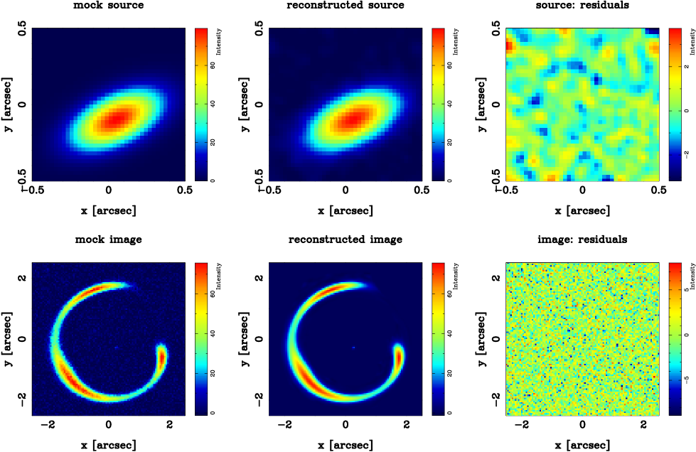
Figure 2.— The left columns presents the simulated source $\vec{s}_{\rm sim}$ and the corresponding lensed image $\vec{d}_{\rm sim}$ with Gaussian noise added. The middle column shows the reconstructed quantities obtained with the lensing operator $\mathbf{L}$ and a particular choice for the regularization. The residuals are shown in the right column.

4. Gravitational lensing

Gravitational lensing can be formulated as the reconstruction of an unknown source brightness distribution $\vec{s}$ (pixelized on a grid composed of $N_{\rm s}$ pixels) given the observed and PSF-convoluted image brightness distribution $\vec{d}$ (sampled on a grid of dimension $N_{\rm d}$). To tackle this problem we have made use of the implementation of the method of non-parametric source reconstruction initially developed by Warren & Dye (2003) and further refined and/or adapted by Treu & Koopmans (2004); Koopmans (2005); Dye & Warren (2005); Suyu et al. (2006); Wayth & Webster (2006); Brewer & Lewis (2006a)

Each pixel $i$ (with $1\leq i\leq N_{\rm d}$) on the image grid, located at position $\vec{x}$, is cast back to the source plane (at position $\vec{y}$) through the lensing equation

$$\vec{y}=\vec{x}-\vec{\alpha}(\vec{x})$$ (12)

where $\vec{\alpha}$ is the deflection angle, calculated from the gravitational potential $\Phi$ as described in Appendix B. Since gravitational lensing conserves the surface brightness $\Sigma$, the equivalence $\Sigma(\vec{y})=\Sigma(\vec{x})$ holds (if the effect of the PSF is neglected). In general, however, $\vec{y}$ will not exactly correspond to the position of a pixel of the fixed source grid. Therefore $\Sigma(\vec{y})$ is expressed as a weighted linear superposition of the surface brightness values at the four pixels $j_{1}\dots j_{4}$ (where the index $j$ runs in the interval $1\dots N_{\rm s}$) which delimit the position $\vec{y}$ (see Treu & Koopmans, 2004). The weights $w_{1}\dots w_{4}$ for each of the source pixels are the bilinear interpolation weights (whose sum adds to unity to conserve flux), and they are stored as the elements $L_{ij_{1}}\dots L_{ij_{4}}$ of a (very) sparse matrix $\mathbf{L}$ of dimension $N_{\rm d}\times N_{\rm s}$, which represents the lensing operator. If the image pixel $i$ is cast outside the borders of the source grid, all the elements of the $i$-th row of $\mathbf{L}$ are put to zero. In case we need to be more accurate, we can split each image grid pixel into $n=n_{1}\times n_{2}$ subpixels and apply the same procedure as before to construct an $n$-factor oversampled lensing matrix of dimension $nN_{\rm d}\times N_{\rm s}$.

The lensing operator is therefore a non linear function of the parameter vector $\vec{\eta}$ through the potential, i.e. $\mathbf{L}=\mathbf{L}(\Phi(\vec{\eta}))$, and must be constructed at each iteration of the cauldron algorithm. From $\mathbf{L}$ we then construct the blurred lensing matrix $\mathbf{M}\equiv\mathbf{B}\mathbf{L}$, where $\mathbf{B}$ is a blurring operator (this is a square matrix of order equal to the number of rows of $\mathbf{L}$) which accounts for the effects of the PSF. If we are dealing with an oversampled lensing matrix, we need to include also a resampling operator $\mathbf{R}$ (of dimension $N_{\rm d}\times nN_{\rm d}$) that sums the oversampled pixels together so that in the end the blurred lensing matrix is defined as $\mathbf{M}\equiv\mathbf{R}\mathbf{B}\mathbf{L}$.

Within this framework, the mapping of the source into the lensed image can be expressed as the set of linear equations (cfr. Eq. [10])

$$\mathbf{M}\vec{s}=\vec{d}.$$ (13)

As discussed in Section 2.1, for Gaussian errors the solution $\vec{s}_{\rm MP}$ of the ill-conditioned linear system from equation (13) is found by minimizing the quadratic penalty function

$$\mathcal{P}_{\rm len}[\vec{s},\Phi(\vec{\eta})]=\frac{1}{2}{(\mathbf{M}\vec{s}-\vec{d})}^{\rm T}\mathbf{C}^{-1}_{\rm L}(\mathbf{M}\vec{s}-\vec{d})+\frac{\lambda_{\rm len}}{2}{||\mathbf{H}\vec{s}||}^{2}$$ (14)

(cf. Eq. [6]) by varying $\vec{s}$ and finding $d\mathcal{P}_{\rm len}/d\vec{s}=0$. Here $\mathbf{C}_{\rm L}$ is the (diagonal) lensing covariance matrix, $\mathbf{H}$ is the lensing regularization matrix, and $\lambda_{\rm len}$ is the corresponding regularization hyperparameter. This problem translates (see again Sect. 2.1) into solving the set of linear equations

$$(\mathbf{M}^{\rm T}\mathbf{C}^{-1}_{\rm L}\mathbf{M}+\lambda_{\rm len}\mathbf{H}^{\rm T}\mathbf{H})\vec{s}=\mathbf{M}^{\rm T}\mathbf{C}^{-1}_{\rm L}\vec{d}$$ (15)

(cf. Eq. [9]).

Although in Eqs. (14) and (15) we have indicated the regularization matrix simply as $\mathbf{H}$ for the sake of clarity, it should be noted that, since $\vec{s}$ represents a two-dimensional grid, it is necessary in practice to consider regularization both in the $x$- and $y$-directions, as described, respectively, by matrices $\mathbf{H}_{x}$ and $\mathbf{H}_{y}$. Therefore, the regularization term in Eq. (15) becomes $\lambda_{\rm len}(\mathbf{H}_{x}^{\rm T}\mathbf{H}_{x}+h^{2}\mathbf{H}_{y}^{\rm T}\mathbf{H}_{y})\vec{s}$, where $h\equiv\Delta x/\Delta y$ is the ratio between the horizontal and vertical pixel scales in the case of “curvature regularization” (see Suyu et al., 2006, for a discussion of different forms of regularization). For a specific description of how the actual regularization matrices are constructed, we refer to Appendix A.

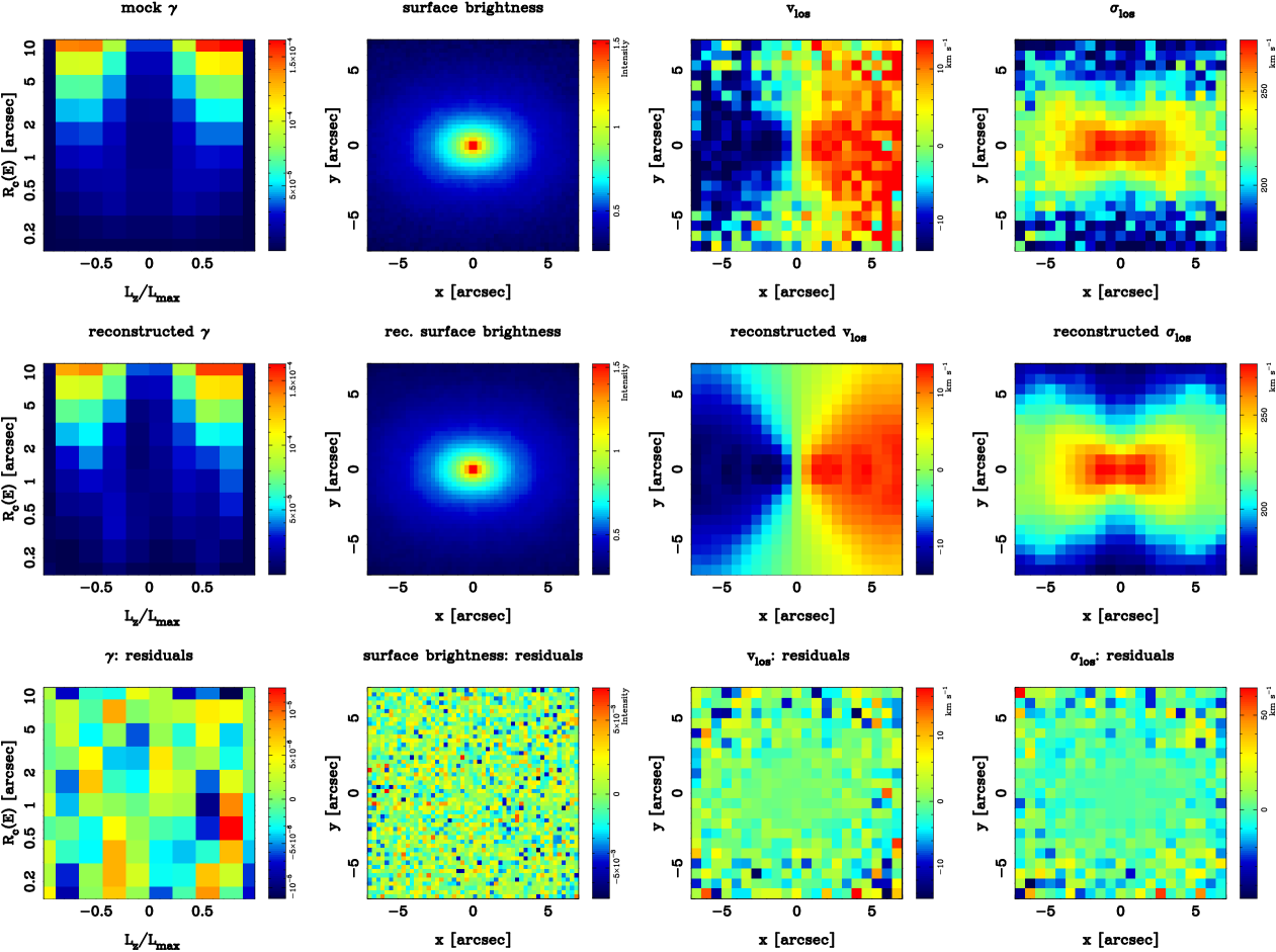
Figure 3.— In the first row we display the weighted distribution function $\vec{\gamma}$ (see text) sampled in the integral space $(E,L_{z})$, together with the set of mock observables generated by this choice (with non-uniform Gaussian noise added): the surface brightness distribution $\Sigma$, the line-of-sight stellar streaming velocity $\langle v_{z^{\prime}}\rangle$ and the line-of-sight velocity dispersion $\sigma^{2}$. The second row shows the corresponding reconstructed quantities. The residuals are given in the last row.

5. Dynamics

In this Section we describe the details of the fast two-integral Schwarzschild method for the dynamical modeling of axisymmetric systems, which is implemented in the cauldron algorithm. It should be noted, however, that Eqs. (16)-(18) are also valid in the general case of arbitrary potentials, provided that $\vec{\gamma}$ is interpreted as the vector of the weights of the different (numerically integrated) stellar orbits of some orbit library. However, the actual construction of the “dynamical operator” $\mathbf{Q}$, as described in Sect. 5.1, is specific to this particular implementation.

As already shown in Sect. 3.1, from a formal point of view the problem of dynamical modeling is identical to that of lensing (Sect. 4), essentially consisting of finding the most probable solution $\vec{\gamma}_{\rm MP}$ for the ill-constrained linear system

$$\mathbf{Q}\vec{\gamma}=\vec{p}$$ (16)

(cf. Eqs.[13] and [10]). Here $\mathbf{Q}$ is the dynamical operator which is applied to the vector $\vec{\gamma}$ of the weights of the building-block $\delta$ distribution functions $f(E,L_{z})$ (the TICs) to generate the set of observables $\vec{p}$. See Sect. 5.1 for a more in-depth description of the meaning of the mentioned quantities and the construction of the matrix $\mathbf{Q}$. As described in Section 2.1, one derives the solution $\vec{\gamma}_{\rm MP}$ by minimizing the quadratic penalty function

$$\mathcal{P}_{\rm dyn}[\vec{\gamma},\Phi(\vec{\eta})] = \frac{1}{2}{(\mathbf{Q}\vec{\gamma}-\vec{p})}^{\rm T}\mathbf{C}^{-1}_{\rm D}(\mathbf{Q}\vec{\gamma}-\vec{p})+$$ (17)

$$\frac{1}{2}\left(\lambda^{\rm dyn}_{L}{||\mathbf{K}_{L}\vec{\gamma}||}^{2}+\lambda^{\rm dyn}_{E}{||\mathbf{K}_{E}\vec{\gamma}||}^{2}\right),$$

which corresponds to solving the set of linear equations

$$(\mathbf{Q}^{\rm T}\mathbf{C}^{-1}_{\rm D}\mathbf{Q}+\lambda^{\rm dyn}_{L}\mathbf{K}_{L}^{\rm T}\mathbf{K}_{L}+\lambda^{\rm dyn}_{E}\mathbf{K}_{E}^{\rm T}\mathbf{K}_{E})\vec{\gamma}=\mathbf{Q}^{\rm T}\mathbf{C}^{-1}_{\rm D}\vec{p}$$ (18)

(note the equivalence with Eqs. (14) and (15) for lensing). Here we have indicated the (diagonal) dynamics covariance matrix as $\mathbf{C}^{-1}_{\rm D}$ and the regularization matrices along the $E$- and $L_{z}$-axes of the $\vec{\gamma}$-grid as $\mathbf{K}_{L}$ and $\mathbf{K}_{E}$, respectively. The regularization along these two directions are (assumed to be) uncorrelated, and the corresponding hyperparameters $\lambda^{\rm dyn}_{L}$ and $\lambda^{\rm dyn}_{E}$ must therefore be considered independently.

With respect to their physical meaning, however, the construction of the linear operators $\mathbf{L}$ and $\mathbf{Q}$ is a markedly distinct problem: the lensing operator describes the distortion to which the source surface brightness distribution is subjected, while the dynamics operator is effectively a library which stores the projected observables (surface brightness distribution and unweighted velocity and velocity dispersion maps) associated with the set of elementary (i.e. Dirac $\delta$) two-integral distribution functions.

5.1. The “dynamics operator” by means of a two-integral axisymmetric Schwarzschild method

In this Section we describe how to construct the dynamics operator $\mathbf{Q}$ (which is the most complex part of implementing Eq. [18] explicitly), introducing a new and extremely fast Monte Carlo implementation of the two-integral components Schwarzschild method, as proposed by Cretton et al. (1999) and Verolme & de Zeeuw (2002). The Schwarzschild method is a powerful and flexible numerical method to construct numerical galaxy models without having to make any prior assumptions regarding the shape, the symmetry, the anisotropy of the system, etc.

In its original implementation (Schwarzschild, 1979), the procedure works as follows. An arbitrary density distribution (possibly motivated by observations) is chosen for the galaxy and the corresponding potential is computed by means of the Poisson equation. One then calculates a library of stellar orbits within this potential and finds the specific superposition of orbits which reproduces the initial density distribution. The method can be generalized to also treat cases in which density and potential are not a self-consistent pair and to include kinematic constraints (see e.g. Richstone, 1980, 1984; Pfenniger, 1984; Rix et al., 1997).

Orbits, however, are not the only possibility for the building blocks of a Schwarzschild method if one only aims to construct two-integral axisymmetric models for galaxies. Given an axisymmetric potential $\Phi(R,z)$, one can also consider more abstract constituents called two-integral components or TICs (see Cretton et al., 1999; Verolme & de Zeeuw, 2002) which correspond to elementary Dirac $\delta$ distribution functions completely specified by a choice of energy $E_{j}$ and angular momentum $L_{z,j}$,

$$f_{j}(E_{j},L_{z,j})=\left\{\begin{array}[]{ll}\displaystyle\frac{\mathcal{C}_{j}}{2}\delta(E-E_{j})\delta(L_{z}-L_{z,j})&\textrm{inside ZVC}\\ &\\ 0&\textrm{elsewhere}\end{array}\right.$$ (19)

where $\mathcal{C}_{j}\equiv\mathcal{C}_{[E_{j},L_{z,j}]}$ is a normalization coefficient chosen such that all the TICs have equal mass (see Appendix D for an explicit expression for $\mathcal{C}_{j}$). The zero-velocity curve (ZVC) is the curve in the meridional plane $(R,z)$ for which

$$E_{\rm kin}=V(R,z)-\frac{L_{z}^{2}}{2R^{2}}-E=0,$$ (20)

where $E$ is the relative energy and $V(R,z)\equiv-\Phi(R,z)$ is the relative potential; another frequently useful quantity is the effective potential $V_{\rm eff}(R,z)=V(R,z)-L_{z}^{2}/2R^{2}$.

A TIC-based Schwarzschild method has two main advantages. First, the $j$-th TIC can be interpreted as a particular combination of all orbits (both regular and irregular, see Cretton et al. 1999) with energy $E_{j}$ and angular momentum $L_{z,j}$ which can be integrated in the potential $\Phi(R,z)$ and completely fill the ZVC. Therefore, the TICs constitute a family of building blocks smoother than the regular orbits (which may have sharp edges) and automatically take into account the irregular orbits. Second, the unprojected density and velocity moments for the TICs have simple analytic expressions, which makes this method much faster than the ordinary orbit integration.

From the definition from equation (19), the density distribution in the meridional plane generated by the $j$-th TIC is given by (see Binney & Tremaine, 1987)

$$\rho_{j}(R,z)=\left\{\begin{array}[]{ll}\displaystyle\frac{\pi\mathcal{C}_{j}}{R}&\textrm{inside ZVC}\\ &\\ 0&\textrm{elsewhere,}\end{array}\right.$$ (21)

while the only non-zero velocity moments have the following expressions inside the ZVC:

$$\rho_{j}\langle v_{\varphi}\rangle_{j}=\frac{\pi\mathcal{C}_{j}}{R^{2}}L_{z,j},$$ (22)

$$\rho_{j}\langle v^{2}_{\varphi}\rangle_{j}=\frac{\pi\mathcal{C}_{j}}{R^{3}}L_{z,j}^{2},$$ (23)

$$\rho_{j}\langle v^{2}_{R}\rangle_{j}=\rho_{j}\langle v^{2}_{z}\rangle_{j}=\frac{\pi\mathcal{C}_{j}}{R}\left[V_{\rm eff}(R,z)-E_{j}\right],$$ (24)

and they vanish elsewhere.

Note that we cannot directly compare the quantities described by Eqs. (21)-(24) with the observations. Before this can be done, we need to calculate the projected quantities, grid them, and convolve them with the appropriate PSF (and possibly regrid them again in the case of subgridding; see text).

The surface brightness $\Sigma_{j}$ (sampled on a grid of $N_{\Sigma}$ elements) and the weighted line-of-sight velocity moments $\Sigma_{j}\langle v_{z^{\prime}}\rangle_{j}$ and $\Sigma_{j}\langle v^{2}_{z^{\prime}}\rangle_{j}$ (both sampled on a grid of $N_{\langle v_{z^{\prime}}\rangle}$ elements) can be obtained semi-analytically through multi-dimensional integrals (refer to Verolme & de Zeeuw, 2002). Because the same semi-analytic approach to calculate $\mathbf{Q}$ is rather time consuming, we have developed a very efficient Monte Carlo implementation of the two-integral Schwarzschild method, detailed in Appendix C, which is several orders of magnitude faster.

Whatever technique is adopted, the projected and PSF-convoluted quantities for the $j$-th TIC, sampled on the appropriate grids, constitute the $j$-th column of the $\mathbf{Q}$ matrix. Therefore, if the galaxy model is built using a library of $N_{\gamma}=N_{E}\times N_{L_{z}}$ TIC building blocks (where $N_{E}$ and $N_{L_{z}}$ are the number of samplings, respectively, in energy and angular momentum), the dynamics operator $\mathbf{Q}$ turns out to be a dense matrix of dimensions $N_{\gamma}\times(N_{\Sigma}+2N_{\langle v_{z^{\prime}}\rangle})$.

The meaning of the vector $\vec{\gamma}$ in Eq. (16) is now clear: its $N_{\gamma}$ dimensionless non negative elements $\gamma_{j}$ describe the weights of the linear superposition of the model observables generated by the library of TICs, and we look for the solution $\vec{\gamma}_{\rm MP}$ (given by Eq. [18]) which best reproduces the data set $\vec{p}$. Moreover, as explained in Appendix D, the weights $\gamma_{j}$ are proportional to the light contributed by the TIC to the galaxy and related to the reconstructed dimensional distribution function $\textrm{DF}(E_{j},L_{z,j})$ when they are normalized with the TIC area $A_{{\rm ZVC},j}$ in the meridional plane and the surface of the cell $A_{[E_{j},L_{z,j}]}$ in integral space.

6. Demonstration of the method

In this Section we describe several of the tests that we have performed to show the proper functioning of the method. We construct a simulated data set (including realistic noise) for both lensing and dynamics by adopting the potential given in Eq. (25) (Evans, 1994) and a particular choice for the non linear parameters $\vec{\eta}$ (see Sect. 6.1 for a description of the setup). Then in Sect. 6.2, keeping the non linear parameters fixed, we test the linear optimization part of the method by showing that the code is able to faithfully reconstruct the source surface brightness distribution and the distribution function used to generate the mock data. Finally, in Sect. 6.3 we execute a full run of the code. We use the mock set of simulated data as input and adopt a starting set of non linear parameters considerably skewed from the “true” values, in order to verify how reliably the linear and non linear parameters are recovered. Note that, for conciseness, what we refer to as the “evidence” $(\mathcal{E})$ is, rigorously speaking, the logarithm of the evidence as presented in Sect. 2. See Appendix E for its precise definition.

6.1. The test setup

As mentioned, for testing purposes it is convenient to make use of the Evans’ power-law potentials (Evans, 1994; Evans & de Zeeuw, 1994)

$$\Phi(R,z)=-\frac{\Phi_{0}R_{\rm s}^{\beta}}{\left(R_{\rm s}^{2}+R^{2}+\displaystyle\frac{z^{2}}{q^{2}}\right)^{\beta/2}}\qquad\beta\neq 0,$$ (25)

where $\Phi_{0}$ is the central potential, $R_{\rm s}$ is a core radius and $q$ is the axis ratio of the equipotentials. For $\beta=0$ this becomes the Binney (1981) logarithmic potential.

What makes this class of axisymmetric galaxy models suitable for the setup of a test case, is the overall simplicity of their properties. The power-law galaxy models are characterized by elementary two-integral distribution functions and provide fully analytical expressions for the density distribution, associated with the potential via the Poisson equation, the second velocity moments and the deflection angle (see Appendix F). Moreover, even the projected quantities (i.e. the projected surface density and the line-of-sight second velocity moment) are analytical. The mean stellar streaming velocity $\langle v_{\varphi}\rangle$ is assigned through a physically motivated prescription (see Sect. 2.3 of Evans & de Zeeuw, 1994) which leads to a simple odd part for the distribution function, which does not contribute to the density and the second velocity moment.

With the choice of the potential from equation (25) for the lens galaxy, the elements of the $\vec{\eta}$ vector of non linear parameters are $\beta$, $q$, $R_{\rm s}$ and $\Phi_{0}$ (or equivalently, through Eq. [B4], the lens strength $\alpha_{0}$). In addition, $\vec{\eta}$ includes the parameters that determine the observed geometry of the system: the inclination $i$, the position angle $\vartheta_{\rm PA}$, and the coordinates $\vec{\xi}_{0}$ of the center of lens galaxy on the sky grid. We note that $\vec{\eta}$ can also include the external shear strength and position angle, although in our current tests we assume negligible shear for the sake of simplicity and to fully concentrate on the parameters of the lens galaxy only, in order to test whether their degeneracies can be broken by the combination of lensing and stellar kinematic data. We also need to make a choice for the size of the grids in pixels. This actually constitutes an explicit prior choice (just like the type of regularization). The evidence however can be used to test exactly these types of assumptions. Explicitly, our test setup is the following.

• Lensing: For the test setup, we adopt a $40\times 40$ pixel grid ($N_{\rm s}=1600$) in the source plane and a $100\times 100$ pixel grid ($N_{\rm d}=10000$) in the image plane. The lensing operator is built using an oversampling factor of $3$ to improve the quality of the reconstruction.

• Dynamics: In the two-integral phase space we consider a grid of $N_{E}=10$ elements logarithmically sampled in $R_{\rm c}(E)$ and $N_{L_{z}}=5$ elements linearly sampled in angular momentum, i.e. a total of $N_{\gamma}=100$ TICs (note that the grid must be mirrored for negative $L_{z}$). Each TIC is populated with $N_{\rm TIC}=10^{5}$ particles. This number of TICs (when compared to the grid size for the lensing source for example) has been verified to be a good compromise between the quality of the distribution function reconstruction and the heavy computational power needed in the iterative scheme for the construction of many TICs. The surface brightness and the line-of-sight velocity moments are sampled on different grids of, respectively, $50\times 50$ and $21\times 21$ elements ($N_{\Sigma}=2500$ and $N_{\langle v_{z^{\prime}}\rangle}=441$). Analogous to the case of lensing, an oversampling factor of $3$ is adopted in the construction of the operator $\mathbf{Q}$.

6.2. Demonstration of the linear reconstruction

We select and fix the following arbitrary (albeit physically plausible) set of values for the $\vec{\eta}$ vector: $\beta=0.28$, $q=0.85$, $R_{\rm c}=0.3^{\prime\prime}$, $\alpha_{0}=4.05^{\prime\prime}$ (and the ratio $D_{\rm ds}/D_{\rm s}$ is taken to be $0.75$), $i=60^{\circ}$, $\vartheta_{\rm PA}=0^{\circ}$ and $\vec{\xi}_{0}=(0.25^{\prime\prime},-0.25^{\prime\prime})$. This makes it possible to construct the lensing operator $\mathbf{M}$ and the dynamics operator $\mathbf{Q}$ (Sects. 4 and 5), which are then used to generate a simulated data set. With a 3 Ghz machine, the construction of the sparse lensing matrix is a very fast process (less than 1 s). Constructing the dynamics operator is more time consuming, although requiring in the above case still only about 7 s, i.e. of the order of 100 ms per TIC (it should be noted that this is a very short time for building a dynamical library and is a direct consequence of the Monte Carlo implementation described in Appendix C.) In addition:

• Lensing: We adopt an elliptical Gaussian source surface brightness distribution $\vec{s}_{\rm sim}$ and using the Evans’ potential from equation (25) (see Eq. [F1] for the analytic expression of the corresponding deflection angle) we generate the blurred lensed image. From this we obtain the final mock image $\vec{d}_{\rm sim}$ by adding a Gaussian noise distribution with $\sigma=0.03$ times the image peak value. This is illustrated in the first column of Fig. 2.

  The reconstruction of the non-negative source $\vec{s}_{\rm rec}$, from the simulated data $\vec{d}_{\rm sim}$, is obtained by solving the linear system of equations (15), with the adoption of a fiducial value for the regularization hyperparameter ($\log\lambda_{\rm len}=-1.0$). Although the matrix $\mathbf{M}^{\rm T}\mathbf{C}^{-1}_{\rm L}\mathbf{M}+\lambda_{\rm len}\mathbf{H}^{\rm T}\mathbf{H}$ in Eq. (15) is large ($10000\times 1600$), it is very sparse and therefore, using L-BFGS-B, it only takes $\lesssim 1$ s to find the solution. The result is shown in Fig. 2 (middle column) together with the residuals (right column).

• Dynamics: We generate the simulated data set $\vec{p}_{\rm sim}$ for a self-consistent dynamical system described by the distribution function of the Evans’ power-law potential. We adopt the same parameters used for the above potential. This kind of assumption, in general, is not required by the method. However, we adopt it here because it immediately and unambiguously allows us to check the correctness of the simulated data in comparison to the analytic expressions. In this way, it is possible to verify that the considered TIC library $\vec{\gamma}_{\rm sim}$, although composed of only $100$ elements, indeed represents a fair approximation of the true distribution function.

  The first two panels in the first row of Fig. 3 show the TIC weights $\vec{\gamma}_{\rm sim}$ (i.e. the weighted distribution function) sampled over the two-integral space grid. The remaining panels display the simulated data: the surface brightness distribution, the line-of-sight streaming velocity and the line-of-sight velocity dispersion As can be seen, non-uniform Gaussian noise has been added to the simulated data (its full characterization is taken into account in the covariance matrix $\mathbf{C}^{-1}_{\rm D}$). The noise on the surface brightness is a few percent of the value of this quantity in the inner region, while, in order to make the test case more realistic, the noise on the velocity moments is increasing outwards and becomes quite severe in the external regions.
  

  The reconstruction of the non negative TIC weights $\vec{\gamma}_{\rm rec}$ is given by the solution of Eq. (18) (the chosen values for the hyperparameters are $\log\lambda^{\rm dyn}_{L}=9.2$ and $\log\lambda^{\rm dyn}_{E}=9.4$). The reconstruction of the dynamical model constitutes, together with the generation of the TIC library, the most time consuming part of the algorithm, requiring almost $10$ s. This is a consequence of the fact that the $3382\times 100$ dynamics operator $\mathbf{Q}$, although much smaller than $\mathbf{L}$, is a fully dense matrix. If the number of TICs is significantly increased, the time required for calculating the term $\mathbf{Q}^{\rm T}\mathbf{C}^{-1}_{\rm D}\mathbf{Q}$ in Eq. (18) and to solve that set of linear equations with the L-BFGS-B method increases very rapidly (as does the time needed to generate the TICs, although less steeply), and therefore the dynamical modeling is typically the bottleneck for the efficiency of the method.

  The results of the reconstruction are shown in the second row of Fig. 3 (whereas the third row shows the residuals). The reconstruction is generally very accurate.

Having verified the soundness of the linear reconstruction algorithms, the next step is to test how reliably the method is able to recover the “true” values of the non linear parameters $\vec{\eta}$ from the simulated data, through the maximization of the evidence penalty function $\mathcal{E}(\vec{\eta})$.

6.3. Non linear optimization

We first run the linear reconstruction for the reference model $\mathcal{M}_{\rm ref}$ described in Sect. 6.2, optimized for the hyper-parameters, to determine the value of the total evidence $\mathcal{E}_{\rm tot,ref}=\mathcal{E}_{\rm len,ref}+\mathcal{E}_{\rm dyn,ref}$ (reported in the first column of Table 1). Since this is by definition the “true” model, it is expected (provided that the priors, i.e. grids and form of regularization, are not changed) that every other model will have a smaller value for the evidence.

Table 1Results for iterative search of the best model parameters via evidence maximization (see text).

		$\mathcal{M}_{\rm ref}$	$\mathcal{M}_{0}$	$\mathcal{M}_{\rm step}$	$\mathcal{M}_{\rm final}$
	$i\;\textrm{[deg]}$	60.0	25.0	75.6	62.6
non linear	$\alpha_{0}$	4.05	5.60	3.86	3.99
parameters	$\beta$	0.280	0.390	0.288	0.285
	$q$	0.850	0.660	0.880	0.857
	$\log\lambda_{\rm len}$	-1.04	0.00	-1.04	-1.04
hyper-	$\log\lambda^{\rm dyn}_{L}$	8.00	12.0	7.99	8.00
parameters	$\log\lambda^{\rm dyn}_{E}$	9.39	12.0	9.55	9.39
	$\mathcal{E}_{\rm len}$	-22663	-58151	-22668	-22661
evidence	$\mathcal{E}_{\rm dyn}$	12738	-156948	12672	12856
	$\mathcal{E}_{\rm tot}$	-9925	-215099	-9996	-9805

The reference model in the second column is the “true” model which generated the simulated data sets, and is shown for comparison. The first group of rows list the non linear parameters $\vec{\eta}$ which are varied in the loop. The second group shows the hyperparameters. The last group shows the evidence relative to the considered model; the contributions of the lensing and dynamics part to the total evidence are also indicated.

Second, we construct a “wrong” starting model $\mathcal{M}_{0}\equiv\mathcal{M}(\vec{\eta}_{0})$ by significantly skewing the values, indicated in the second column of Table 1, of the four non linear parameters: the inclination $i$, the lens strength $\alpha_{0}$, the slope $\beta$ and the axis ratio $q$. Figures 4 and 5 show that $\mathcal{M}_{0}$ is clearly not a good model for the data in hand. We do not set boundaries on the values that the non linear parameters can assume during the iterative search, except for those which come from physical or geometrical considerations (i.e. inclination comprised between edge-on and face-on, $\alpha_{0}\geq 0$, $0\leq q\leq 1$, $0<\beta\leq 1$). The position angle, in general, is reasonably well-constrained observationally, and therefore including it with tight constraints on the interval of admitted values would only slow down the non linear optimization process without having a relevant impact on the overall analysis. It is therefore kept fixed during the optimization. We also keep the core radius of the mass distribution fixed even though in general it is not well constrained by the surface brightness distribution and in real applications it should be varied. It always remains possible, once the best model has been found, to optimize for the remaining parameters in case a second-order tuning is required.

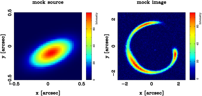
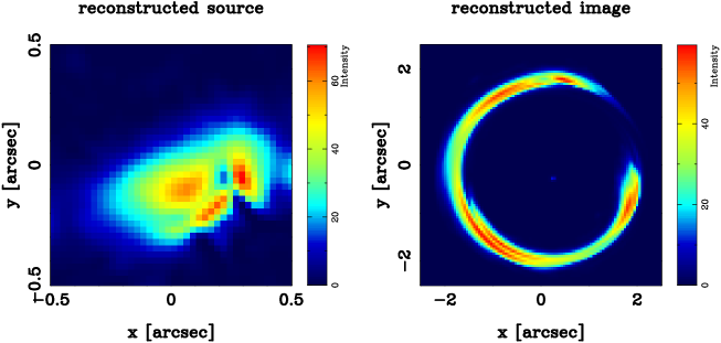
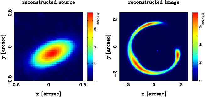
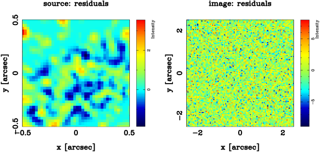
Figure 4.— Outcome of the non linear optimization routine for the lensing block. The first row shows the simulated source and lensed image. In the second row is the starting model $\mathcal{M}_{0}$ obtained with the skewed parameters, which clearly produces a poor reconstruction of the image (hence the very low value of the evidence). The third row displays the final model $\mathcal{M}_{\rm final}$, that is the “best model” recovered through the non linear optimization for evidence maximization. This should be compared to the reference model $\mathcal{M}_{\rm ref}$ (i.e. generated with same $\vec{\eta}$ set of parameters which were used to generate the mock data), presented in the second column of Fig. 2. The last row shows the residuals of the final model when compared to the simulated data. Refer to Table 1 for the non linear parameters and hyperparameters of the models and the corresponding value of the evidence.

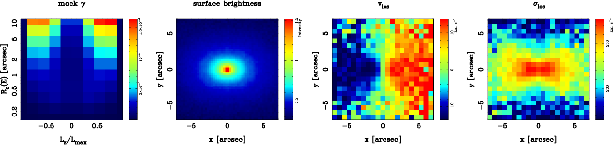
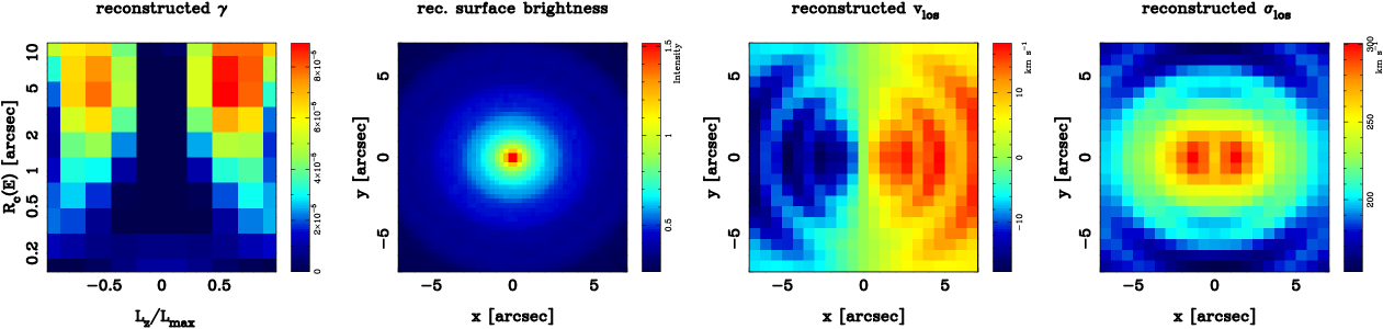
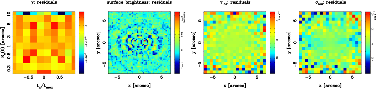
Figure 5.— Outcome of the non linear optimization routine for the dynamics block. The first row shows the simulated set of TIC weights $\vec{\gamma}$ (i.e. the weighted distribution function) in the integral space and the resulting observables: the surface brightness $\Sigma$, the line-of-sight streaming velocity $\langle v_{z^{\prime}}\rangle$ and the line-of-sight velocity dispersion $\sigma^{2}_{\rm los}$. The second row presents the reference model $\mathcal{M}_{\rm ref}$ (i.e. generated with same $\vec{\eta}$ set of parameters which were used to generate the mock data). In the second row is the starting model $\mathcal{M}_{0}$ obtained with the skewed parameters, which produces a poor reconstruction of the observables, in particular the velocity moments. The third row displays the final model $\mathcal{M}_{\rm final}$, that is the “best model” recovered through the non linear optimization for evidence maximization. This should be compared to the reference model $\mathcal{M}_{\rm ref}$ (i.e. generated with same $\vec{\eta}$ set of parameters which were used to generate the mock data), presented in the second row of Fig. 5. The last row shows the residuals of the final model when compared to the simulated data. Refer to Table 1 for the non linear parameters and hyperparameters of the models and the corresponding value of the evidence.

Adopting $\vec{\eta}_{0}$ as the starting point for the exploration, the non linear optimization routine for the evidence maximization is run as described in Sect. 2.2. The model $\mathcal{M}_{\rm step}$ (third column of Table 1) is what is recovered after three major loops (the first and the last one for the optimization of the varying non linear parameters, the intermediate one for the hyperparameters) of the preliminary Downhill-Simplex optimization, for a total of $\sim 1000$ iterations, requiring about $1.2\times 10^{4}$ s on a 3 Ghz machine. From this intermediate stage, the final model $\mathcal{M}_{\rm final}$ is obtained through the combined MCMC+Downhill-Simplex optimization routine, in a time of the order of $12-15$ hours.

Further testing has shown that increasing the number of loops does not produce relevant changes in the determination of the non linear parameters nor of the hyperparameters, and therefore extra loops are in general not necessary. We also note that, in all the considered cases, the first loop is the crucial one for the determination of $\vec{\eta}$, and the one which requires the largest number of iterations before it converges. It is generally convenient to set the initial hyperparameters to high values so that the system is slightly over-regularized. This has the effect of smoothing the evidence surface in the $\vec{\eta}$-space, and, therefore, facilitates the search for the maximum. The successive loops will then take care of tuning down the regularization parameters to more plausible values.

Figure 6.— These plots show how the degeneracy between different lens models is broken when the constraints given by the stellar dynamics are also considered. The three panels display a cut through the surfaces of, respectively, lensing evidence, dynamics evidence and total evidence. The abscissa coordinate $\epsilon$ represents a series of different $\vec{\eta}$ sets, i.e. different models, obtained as a linear interpolation between the model parameters $\vec{\eta}_{\epsilon=0}\equiv$ ($i=35\arcdeg$, $\alpha=5.59$, $\beta=0.297$, $q=0.602$), i.e. the best model which is obtained by maximizing for lensing evidence only, and the model $\vec{\eta}_{\epsilon=1}$ which is the reference model $\mathcal{M}_{\rm ref}$ of Table 1. As far as only the gravitational lensing is considered, the two maxima in the evidence are effectively degenerate, with the “wrong” model $\vec{\eta}_{\epsilon=0}$ being slightly preferred ($\Delta\mathcal{E}_{\rm len}=2$). When the contribution of the evidence of dynamics is considered, however, the degeneracy is broken and the reference model emerges as indisputably favored by the total evidence ($\Delta\mathcal{E}_{\rm tot}\simeq 35000$).

A comparison of the retrieved non linear parameters for $\mathcal{M}_{\rm final}$ (last column of Table 1) with the corresponding ones for the reference model reveals that all of them are very reliably recovered within a few percent (the most skewed one is the inclination $i$, being only $\sim 4\%$ different from the “true” value). The panels in the second and fourth rows of Figures 4 and 5 clearly show that the two models indeed look extremely similar, to the point that they hardly exhibit any difference when visually examined.

The evidence of the final model, when compared with the value for the reference model, turns out to be higher by $\Delta\mathcal{E}\equiv\mathcal{E}_{\rm final}-\mathcal{E}_{\rm ref}=120$, which might look surprising since $\mathcal{M}_{\rm ref}$ is by construction the “true” model. The explanation for this is given by the cumulative effects of numerical error (which enters mainly in the way the TICs are generated), finite grid size, and noise (in particular on the velocity moments), which all contribute to slightly shift the model. Such a shift is, however, well within the model uncertainties (Sect. 6.4) and therefore not significant.

6.3.1 Degeneracies and Biases

Extensive MCMC exploration reveals that the lensing evidence surface $\mathcal{E}_{\rm len}(\vec{\eta})$ is characterized by multiple local maxima which effectively are degenerate even for very different values of $\vec{\eta}$. Indeed, for the potential Eq. (25), one can easily observe from Eq. (F1) that a relation between $q$, $i$, and $\Phi_{0}$ exists that leaves the deflection angles and, hence, the lens observable invariant.

In this situation, the dynamics plays a crucial role in breaking the degeneracies and reliably recovering the best values for the non linear parameters. A clear example is shown in Figure 6, where cuts along the evidence surfaces are presented. The left panel of Figure 6 displays two almost degenerate maxima in $\mathcal{E}_{\rm len}$; indeed, the maximum located at the linear coordinate $\epsilon=0$ (corresponding to the set of non linear parameters $i=35\arcdeg$, $\alpha=5.59$, $\beta=0.297$, $q=0.602$) has a value for the lensing evidence of $-22661$, and therefore, judging on lensing alone, this model would be preferred to the reference model (see Table 1) which corresponds to the other maximum at $\epsilon=1$. When the evidence of the dynamics (Fig. 6 central panel) is considered, however, the degeneracy is broken and the “false” maximum is heavily penalized with respect to the true one, as shown by the resulting total evidence surface (Fig. 6 right panel).

Test cases with a denser sampling of the integral space (e.g. $N_{E}\times N_{L_{z}}=12\times 8$, $18\times 9$, $20\times 10$) were also considered. This analysis revealed that, although one obtains more detailed information about the reconstructed two-integral distribution function at the cost of a longer computational time (e.g. in the $18\times 9$ case the loop phase is slower by more than a factor of 2), the accuracy of the recovered non linear parameters – which is what we are primarily interested in – does not (significantly) improve. As a consequence, the $N_{\gamma}=100$ case is assumed to be the standard grid for the integral space as far as the dynamical modeling is concerned to give an unbiased solution. Once the non linear parameters have been recovered through the evidence maximization routine, it is possible to start from the obtained results to make a more detailed and expensive study of the distribution function using a higher number of TICs.

6.4. Model uncertainties

To determine the scatter in the recovered parameters $\vec{\eta}$ we performed the full non linear reconstruction on a set of ${100}$ random realizations of the test data. The statistical analysis of the results is summarized in Table 2. On examining the $95\%$ confidence intervals, the parameters appear to be quite tightly constrained, with the partial exception of the inclination angle which spans an interval of approximately $10^{\circ}$. The means (and the medians) of the parameters $\alpha$, $\beta$ and $q$ are very close to the “true values” of the reference model, while the mean of parameter $i$ is slightly more skewed. The two sets of parameters ($i$, $q$) and ($\alpha$, $\beta$) are clearly significantly correlated when plotted against each other (see Fig. 7 for a graphical representation of the correlation matrix). Both correlations can be understood. The former is due to the fact that the projected lens potential is nearly invariant when the inclination is increased and flattening is decreased simultaneously; whereas, in the latter case the requirement that the lens mass enclosed by the lensed images be very similar between lens models causes the lens strength and density slopes to vary in concordance.

Although the starting parameters of model $\mathcal{M}_{0}$ are very different from the “true” solution given by $\mathcal{M}_{\rm ref}$, in all the considered cases the recovered parameters end up close to the $\mathcal{M}_{\rm ref}$ ones, and there is no case in which the solution remains anchored in a really far-off local minimum. Hence, even in the case of our chosen lens potential, which has global degeneracies in the lensing observables (see Section 6.3.1), these degeneacies are broken through the inclusion of stellar kinematic data. This indeed shows that the combination of lensing and stellar kinematic information is a very promising tool to break degeneracies of the galaxy mass models.

Table 2Summary of the results of the non linear reconstruction algorithm applied on a set of ${100}$ random realizations of the test data.

		median	mean	$95\%$ C.I.	$\mathcal{M}_{\rm ref}$
	$i\;\textrm{[deg]}$	63.0	63.3	[59.5, 69.5]	60.0
non linear	$\alpha_{0}$	4.02	4.02	[3.94, 4.10]	4.05
parameters	$\beta$	0.276	0.277	[0.266, 0.293]	0.280
	$q$	0.861	0.861	[0.849, 0.873]	0.850

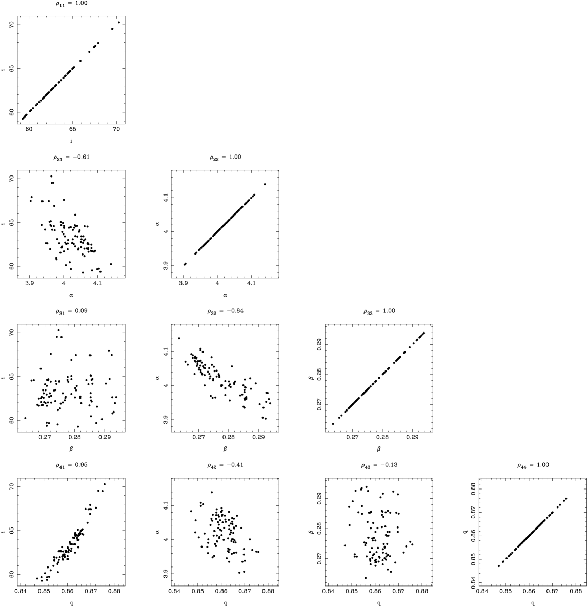
Figure 7.— Graphical visualization of the lower triangle of the (symmetric) correlation matrix for the parameters recovered from the non linear reconstruction of ${100}$ random realizations of the test data. In the shown panels the four non linear parameters $i$, $\alpha$, $\beta$ and $q$ are plotted two by two against each other; for each panel, the corresponding value $\rho_{ij}$ of the correlation matrix is also indicated.

7. Conclusions and future work

We have presented and implemented a complete framework to perform a detailed analysis of the gravitational potential of (elliptical) lens galaxies by combining, for the first time, in a fully self-consistent way both gravitational lensing and stellar dynamics information.

This method, embedded in a Bayesian statistical framework, enables one to break to a large extent the well-known degeneracies that constitute a severe hindrance to the study of the early-type galaxies (in particular those at large distances, i.e. $z\gtrsim 0.1$) when the two diagnostic tools of gravitational lensing and stellar dynamics are used separately. By overcoming these difficulties, the presented methodology provides a new instrument to tackle the major astrophysical issue of understanding the formation and evolution of early-type galaxies.

The framework is very general in its scope and in principle can accommodate an arbitrary (e.g. triaxial) potential $\Phi(\vec{x})$. In fact, if a combined set of lensing data (i.e. surface brightness distribution of the lensed images) and kinematic data (i.e. surface brightness distribution and velocity moments maps of the galaxy) is provided for an elliptical lens galaxy, it is always possible, making use of the same potential, to formulate the two problems of lensed-image reconstruction and dynamical modeling as sets of coupled linear equations to which the linear and non linear optimization techniques described in Sect. 3 and 2 can be directly applied.

More specifically, in the case of gravitational lensing the non-parametric source reconstruction method (as illustrated in Sect. 4) straightforwardly applies to the general case of any potential $\Phi(\vec{x})$. In the case of dynamical modeling, a full Schwarzschild method with orbital integration would be required; this would constitute, however, only a mere technical complication which does not modify the overall conceptual structure of the method.

7.1. The cauldron algorithm

In practical applications, however, technical difficulties and computational constraints must also be taken into account. This has motivated the development, from the general framework, of the specific working implementation described in this paper, which restricts itself to axisymmetric potentials $\Phi(R,z)$ and two-integral stellar phase-space distribution functions. This choice is an excellent compromise between efficiency and generality. On one hand it allows one to study models which go far beyond the simple spherical Jeans-modeling case, and on the other hand, it has the invaluable advantage of permitting a dynamical modeling by means of the two-integrals Schwarzschild method of Verolme & de Zeeuw (2002). This method (see Sect. 5) is based on the superposition of elementary building blocks (i.e. the TICs) directly obtained from the two-integral distribution function, which do not require computationally expensive orbit integrations.

More specifically, we have sped up this method by several orders of magnitude by designing a fully novel Monte Carlo implementation (see Appendix C). Hence, we are now able to construct a realistic two-integral dynamical model and its observables (surface brightness and line-of-sight projected velocity moments) in a time of the order of $5-15$ s on a typical 3 Ghz machine.

The Bayesian approach (e.g. Sect. 2) constitutes a fundamental aspect of the whole framework. On a first level, the maximization of the posterior probability, by means of linear optimization, provides the most probable solution for a given data set and an assigned model (which will be, in general, a function of some non linear parameters $\vec{\eta}$, e.g. the potential parameters, the inclination, the position angle) in a fast and efficient way. A solution (i.e. the source surface brightness distribution for lensing and the distribution function for dynamics), however, can be obtained for any assigned model. The really important and challenging issue is instead the model comparison, that is, to objectively determine which is the “best” model for the given data set or, in other words, which is the “best” set of non linear parameters $\vec{\eta}$. Bayesian statistics provides the tool to answer these questions in the form of a merit function, the “evidence”, which naturally and automatically embodies the principle of Occam’s razor, penalizing not only mismatching models but also models which correctly predict the data but are unnecessarily complex (e.g. MacKay, 1992, 1999; Mackay, 2003). The problem of model comparison thus becomes a non linear optimization problem (i.e. maximizing the evidence), for which several techniques are available (see Sect. 2.2).

As reported in Sect. 6, we have conducted successful tests of the method, demonstrating that both the linear reconstruction and the non linear optimization algorithms work reliably. It has been shown that it is possible to recover within a few percent the values of the non linear parameters of the reference model (i.e. the “true” model used to generate the simulated data set), even when starting the reconstruction from a very skewed and implausible (in terms of the evidence value) initial guess for the non linear parameters. Such an accurate reconstruction is a direct consequence of having taken into account, beyond the information coming from gravitational lensing, the constraints from stellar dynamics. Indeed, when the algorithm is run considering only the lensing data, degenerate solutions with comparable or almost coincident values for the evidence are found, making it effectively impossible to distinguish between these models. The crucial importance of the information from dynamics is exhibited by the fact that, when it is included in the analysis, the degeneracies are fully broken and a solution very close to the true one is unambiguously recovered (see Fig. 6 for an example).

Bearing in mind these limitations and their consequences, however, it should also be noted that the full modularity of the presented algorithm makes it fit to be used also in those situations in which either the lensing or the kinematic observables are not available. This would allow one, for example, to restrict the plausible models to a very small subset of the full space of non linear parameters, although a single non-degenerate “best solution” would probably be hard or impossible to find.

7.2. Future work

Eventhough the methodology that we introduced in this paper works very well and is quite flexible, we can foresee a number of improvements for the near and far future, in order of perceived complexity. (i) Exploration of the errors on the non linear parameters $\vec{\eta}$ through a MCMC method, even though this requires an extension of the MCMC framework in the context of the Bayesian evidence, since one also needs to explore variations in the lens parameters due to changes in the hyperparameters, and not only changes in the posterior for fixed hyperparameters. (ii) Implementation of additional potential (or density) models or even a non-parametric or multi-pole expansion description of the gravitational potential in the $(R,z$)-plane for axisymmetric models. This allows more freedom for the galaxy potential description. (iii) Implementing an approximate three-integral method in axisymmetric potentials (e.g. Dehnen & Gerhard, 1993). (iv) Including an additional iterative loop around the posterior probability optimization, one can construct stellar phase-space distribution functions that are self-consistent, i.e. they generate the potential for which they are solutions to the collisionless Boltzmann equation. This would allow the stellar and dark-matter potential contributions to be separated, a feature not yet part of the current code. (v) A full implementation of Schwarzschild’s method for arbitrary potentials through orbital integration.

Besides these technical improvements, which are all beyond the scope of this methodological paper, we also plan, in a future publication, a set of additional performance tests to see to what level each of the degeneracies (e.g. the mass sheet and mass anisotropy) in lensing and stellar dynamics are broken and how far the simpler lensing plus spherical Jeans approach (e.g. Treu & Koopmans, 2004; Koopmans et al., 2006) gives (un)biased results. Such studies would allow us to better interpret the results obtained in cases where spatially resolved stellar kinematics is not available (e.g. for faint very high redshift systems; Koopmans & Treu, 2002).

As for the application, the algorithm described in this paper will be applied in a full and rigorous analysis of the SLACS sample of massive early-type lens galaxies (see Bolton et al., 2006; Treu et al., 2006; Koopmans et al., 2006) for which the available data include Hubble Space Telescope Advanced Camera for Survey and NICMOS images of the galaxy surface brightness distribution and lensed image structure and maps of the first and second line-of-sight projected velocity moments (obtained with VLT-VIMOS two-dimensional integral field spectroscopy, as part of the Large Program and as a series of Keck long-slit spectra).

Appendix A Regularization

We make use of a curvature regularization. This form of regularization tries to put the second derivative between a pixel and the two adjacent ones to zero and has been shown by Suyu et al. (2006) to be optimal for the reconstruction of smooth distributions. The curvature regularization has been chosen since we do not expect, in the majority of cases, to have sharp intensity variations in the surface brightness distribution of an extended source (for lensing) or in the distribution function of a galaxy. However, other choices of regularization can easily be implemented and ranked according to their evidence (Suyu et al., 2006).

Following the notation of Sect. 2, we indicate as $\vec{x}$ the linear parameter vector (or, more simply, the source) and as $\mathbf{H}$ the regularization matrix. Since the source is defined on a rectangular grid of $N=N_{\rm row}\times N_{\rm col}$ elements, $\mathbf{H}$ actually consists of two matrices, $\mathbf{H}_{\rm row}$ and $\mathbf{H}_{\rm col}$, which regularize the grid pixels along the rows and the columns, respectively. The horizontal regularization operator $\mathbf{H}_{\rm row}$ is a square matrix of rank $N$. In each row $i$ the only non zero elements are $h_{i,i-1}=+1,h_{i,i}=-2,h_{i,i+1}=+1$; the only exceptions are the rows $1+kN_{\rm col}$ and $N_{\rm col}+kN_{\rm col}$ (with $k=0,1,\dots,N_{\rm row}-1$), where a zeroth-order regularization is performed (i.e. $h_{i,i}=1$ is the only non zero term) to prevent the connection of pixels belonging to different rows which are therefore physically uncorrelated. Similarly, the vertical regularization operator $\mathbf{H}_{\rm col}$ is constructed such that in each row $i$ all the elements are zero with the exclusion of $h_{i,i-N_{\rm col}}=+1,h_{i,i}=-2,h_{i,i+N_{\rm col}}=+1$; a zeroth-order regularization is applied for the rows $1\dots N_{\rm col}$ and $N-N_{\rm col}+1\dots N$.

Appendix B Normalization: setting the scale of lensing

For the assigned three-dimensional gravitational potential $\Phi$, the reduced deflection angle $\vec{\alpha}$ is given by (e.g. Schneider, Ehlers, & Falco, 1992)

$$\vec{\alpha}(x^{\prime},y^{\prime})=\frac{2}{c^{2}}\frac{D_{\rm ds}}{D_{\rm s}}\int_{-\infty}^{+\infty}\nabla_{\vec{\xi}}\Phi(\vec{\xi},z^{\prime})\,{\rm d}z^{\prime},$$ (B1)

where $z^{\prime}$ is the line-of-sight coordinate, $(x^{\prime},y^{\prime})\equiv\vec{\xi}$ are the sky coordinates and $\nabla_{\vec{\xi}}$ denotes the two-dimensional gradient operator in the plane of the sky; $c$ is the speed of light expressed in the same units as the value of ${|\Phi|}^{1/2}$. If the gradient operator, which does not depend on $z^{\prime}$, is taken out of the integral and the potential is conveniently written as

$$\Phi(\vec{\xi},z^{\prime})=\Phi_{0}\times\tilde{\Phi}(\tilde{\vec{\xi}},\tilde{z}^{\prime}),$$ (B2)

where $\Phi_{0}$ is the normalization constant in the most suitable physical unit (in our case km s^-1) and $\tilde{\Phi}$ is a function of the dimensionless coordinates expressed as angles in arcseconds ($\tilde{\vec{\xi}}\equiv\frac{648000}{\pi}\vec{\xi}/D_{\rm d}$, $\tilde{z}^{\prime}\equiv\frac{648000}{\pi}z^{\prime}/D_{\rm d}$), then the deflection angle assumes the expression

$$\vec{\alpha}(\tilde{x}^{\prime},\tilde{y}^{\prime})=\alpha_{0}\,\nabla_{\tilde{\vec{\xi}}}\left[\int_{-\infty}^{+\infty}\tilde{\Phi}(\tilde{\vec{\xi}},\tilde{z}^{\prime})\,{\rm d}z^{\prime}\right],$$ (B3)

where

$$\alpha_{0}\equiv\frac{6.48\times 10^{5}}{\pi}\frac{2\Phi_{0}}{c^{2}}\frac{D_{\rm ds}}{D_{\rm s}}$$ (B4)

is the lens strength in arcseconds. The parameter $\alpha_{0}$ sets the scale for the lensing and, therefore, is always included in the parameter vector $\vec{\eta}$. Eq. (B4) openly displays how intimately the lens strength is connected to the normalization of the three-dimensional potential (the same used for the dynamical modeling) within our joint method.

Appendix C A MCMC implementation of the two-integral axisymmetric Schwarzschild method

In this Appendix we describe the numerical implementation of the two-integral axisymmetric Schwarzschild method of Verolme & de Zeeuw (2002) that we developed to significantly accelerate the construction of the dynamical model, i.e. the projected and PSF-convoluted model observables generated by the TIC library.

As a first step, we construct a library composed of $N_{\gamma}=N_{E}\times N_{L_{z}}$ TICs in the given potential $\Phi$ (here $N_{L_{z}}$ is an even number). We consider a grid (linear or logarithmic) in the circular radius $R_{\rm c}$ with $N_{E}$ samplings between $R_{\rm c,min}$ and $R_{\rm c,max}$. The range is chosen to include most of the mass or, if the mass is infinite for the potential $\Phi$, to provide a satisfactory sampling of the potential profile in the radial direction. For each $R_{\rm c}$ the circular speed $v_{\rm c}$ is calculated as

$$v_{\rm c}^{2}(R_{\rm c})=R_{\rm c}\left.\frac{\partial\Phi}{\partial R}\right|_{(R_{\rm c},0)}$$ (C1)

and the angular momentum of the circular orbit $L_{z,{\rm max}}=R_{\rm c}v_{\rm c}$ is set. Computing the energy $E_{\rm c}\equiv E(R_{\rm c})=V_{\rm eff}(R_{\rm c},0)$ of the circular orbit at $R_{\rm c}$, the radial grid is immediately translated into a sampling in energy. For each value of $E_{\rm c}$, the grid in the normalized angular momentum $\eta\equiv L_{z}/L_{z,{\rm max}}$ is constructed by sampling (linearly or logarithmically) $N_{L_{z}}/2$ values between the minimum $\eta_{\rm min}=0$ and the maximum $\eta_{\rm max}=1$. (For numerical reasons, the grid is actually not sampled between these extrema, but between $\eta_{\rm min}=\epsilon$ and $\eta_{\rm max}=1-\epsilon$, with $\epsilon\ll 1$). To take the odd part of the distribution function into account as well, we likewise consider the $N_{L_{z}}/2$ negative values for the angular momentum, $\eta=-1\dots\eta=0$, on a mirror grid.

We also need to define a suitable coordinate frame for the galaxy. Since the system is axisymmetric, we adopt the cylindrical coordinates $(R,\varphi,z)$, with the origin on the center of the galaxy. If the galaxy is observed at an inclination $i$ and $\vartheta_{\rm PA}$ is the position angle (defined as the angle measured counterclockwise between the north direction and the projected major axis of the galaxy), the projected coordinates $(x^{\prime},y^{\prime},z^{\prime})$ are given by

$$\left\{\begin{array}[]{l}x^{\prime}=R(\cos\vartheta_{\rm PA}\sin\varphi+\sin\vartheta_{\rm PA}\cos i\cos\varphi)-z\sin\vartheta_{\rm PA}\sin i\\ \\ y^{\prime}=R(\sin\vartheta_{\rm PA}\sin\varphi-\cos\vartheta_{\rm PA}\cos i\cos\varphi)+z\cos\vartheta_{\rm PA}\sin i\\ \\ z^{\prime}=R\sin i\cos\varphi+z\cos i.\end{array}\right.$$ (C2)

Here $z^{\prime}$ is measured along the line of sight, while $x^{\prime}$ and $y^{\prime}$ are in the plane of sky and are directed (respectively) along the projected major and minor axes of the galaxy.

For any TIC, we populate the surface inside the zero velocity curve with $N_{\rm TIC}$ particles of mass (or equivalently luminosity) $m$ by means of a Markov-Chain Monte Carlo routine whose probability distribution is given by Eq. (21) for the density. This effectively corresponds to numerically reproducing the density $\rho(R,z)$, fixing at the same time the total mass $M_{\rm TIC}=mN_{\rm TIC}$ for each TIC. However, since $\rho(R,z)\propto 1/R$, the surface density of the torus “wrapped” onto the meridional plane (denoted as $\varsigma$) is constant, i.e.,

$$\varsigma_{j}(R,z)\equiv\int_{0}^{2\pi}\rho_{j}(R,z)R{\rm d}\varphi=\left\{\begin{array}[]{ll}2\pi^{2}\mathcal{C}_{j}&\textrm{inside ZVC}\\ &\\ 0&\textrm{elsewhere}.\\ \end{array}\right.$$ (C3)

One can take advantage of this property to greatly simplify the Markov-Chain Monte Carlo routine. Now it is only necessary to uniformly populate the meridional plane. For each particle a pair of coordinates $(R,z)$ (within some interval which encompasses the ZVC) is randomly generated. If it falls outside the ZVC, the particle is “rejected” and another one is generated. If the coordinates are located inside the ZVC, a random value in the interval $[0,2\pi)$ is chosen for the azimuthal coordinate in order to have a complete tern $(R,\varphi,z)$, and the particle counts toward the total of $N_{\rm TIC}$ drawings. This procedure yields at the same time the surface $A_{{\rm ZVC},j}$ enclosed by the ZVC in the meridional plane (effectively obtained via Monte Carlo integration), which is required for the normalization of the $\gamma_{j}$ (see Appendix D).

With this method the computation of all the projected quantities is fast and straightforward. For each “accepted” mass point we know the cylindrical coordinates $(R,\varphi,z)$; associated with it are also the velocity moments defined by Eqs. (22)-(24). Using the first two equations of the transformation from equation (C2), the projected coordinates $(x^{\prime},y^{\prime})$ are directly calculated. Casting the points on a grid on the sky plane and summing up all the points in the same pixel then reproduces numerically the projected surface brightness distribution $\Sigma_{j}$ (see Figure 8 for an illustration). The line-of-sight velocity moments associated with each point in the sky plane (but possibly on a different grid) are obtained in an analogous way (but making use now of the third equation of [C2]) from the corresponding unprojected quantities

$$\langle v_{z^{\prime}}\rangle=-\langle v_{\varphi}\rangle\sin i\sin\varphi,$$ (C4)

$$\langle v^{2}_{z^{\prime}}\rangle=\left(\langle v^{2}_{R}\rangle\cos^{2}\varphi+\langle v^{2}_{\varphi}\rangle\sin^{2}\varphi\right)\sin^{2}i+\langle v^{2}_{R}\rangle\cos^{2}i.$$ (C5)

In analogy with the surface brightness, the first and second line-of-sight moments associated with each mass point inside a given pixel are summed up. This gives the quantities $\Sigma\langle v_{z^{\prime}}\rangle$ and $\Sigma\langle v^{2}_{z^{\prime}}\rangle$.

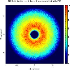
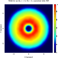
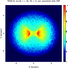
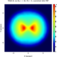
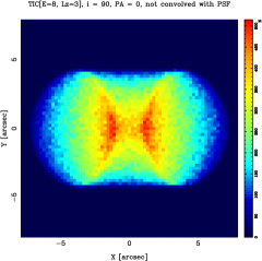
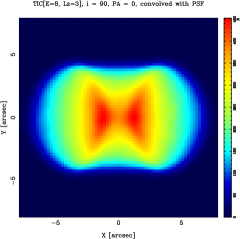
Figure 8.— As an illustration of the method described in the text, we show for a given TIC (obtained with $N_{\rm TIC}=5\times 10^{5}$ particles) the density distribution projected, from top to bottom, at $i=0\arcdeg$ (face-on), $i=45\arcdeg$, and $i=90\arcdeg$ (edge-on). In the left column the density distribution is not convolved with the PSF; in the right column it is convolved with a Gaussian PSF of standard deviation $\sigma_{x}=\sigma_{y}=0.10\arcsec$.

The effect of the PSF is taken into account by simply convolving the projected surface brightness or weighted velocity moments calculated on their respective grids (preferably oversampled) with the PSF profile sampled on the same grid. This operation can be numerically performed in a very efficient way through several FFTs (fast Fourier transforms).

This numerical implementation is dramatically faster than the semi analytic approach (at the expense of some numerical noise). On a machine with a 3 Ghz processor, the whole process of calculating the projected quantities $\Sigma$, $\langle v_{z^{\prime}}\rangle$, and $\langle v^{2}_{z^{\prime}}\rangle$ convolved with the PSF for 1400 TICs takes about 3 minutes (with $N_{\rm TIC}=10^{5}$). This figure should be compared with the $\sim 30$ minutes required by Verolme & de Zeeuw (2002) to calculate (on a 1 GHz machine) only the projected density without PSF convolution for an equal number of TICs.

Appendix D Normalization of the TICs weights

In this Appendix we illustrate how the reconstructed adimensional weights $\gamma_{j}$ are translated into the dimensional distribution function values $\textrm{DF}(E_{j},L_{z,j})$. For a two-integral distribution function, the density is given by the formula (e.g. Binney & Tremaine, 1987)

$$\varsigma(R,z)=2\pi R\rho(R,z)=4\pi^{2}\int_{0}^{V}{\rm d}E\int_{L_{z}^{2}<2(V-E)R^{2}}\textrm{DF}(E,L_{z}){\rm d}L_{z},$$ (D1)

where $\varsigma(R,z)$ is the surface density “wrapped” in the meridional plane (cf. definition [C3]). If we assume that DF can be considered approximately constant over the cell ${\rm d}E_{j}{\rm d}L_{z,j}$ of area $A_{[E_{j},L_{z,j}]}$ in the integral space, and we remember the properties of the TICs, then we have

$$4\pi^{2}\textrm{DF}(E_{j},L_{z,j}){\rm d}E_{j}{\rm d}L_{z,j}=\gamma_{j}\varsigma_{j}(R,z).$$ (D2)

In the previous formula, $\varsigma_{j}$ is the “wrapped” surface density generated by $\textrm{TIC}_{j}$, specified by the pair $(E_{j},L_{z,j})$, which is constant inside the ZVC and zero elsewhere (see Eq. [C3]):

$$\varsigma_{j}=2\pi^{2}\mathcal{C}_{j}=\frac{M_{\rm TIC}}{A_{{\rm ZVC},j}}\qquad\textrm{(inside the ZVC)};$$ (D3)

here $A_{{\rm ZVC},j}$ denotes the area enclosed by the ZVC in the meridional plane (which can be calculated as described in Appendix C) and $M_{\rm TIC}=mN_{\rm TIC}$ is the fixed TIC mass (all the TICs have equal mass by construction).

Combining Eqs. (D2) and (D3) we find the desired relation

$$\textrm{DF}(E_{j},L_{z,j})=\gamma_{j}\frac{mN_{\rm TIC}}{4\pi^{2}A_{{\rm ZVC},j}A_{[E_{j},L_{z,j}]}},$$ (D4)

which translates the weights $\gamma_{j}$ into distribution function values expressed in the standard physical units of mass length^-3 velocity^-3. If $m$, in the numerator of the right-hand side of Eq. (D4), is omitted or divided by a mass-to-light ratio coefficient $\Gamma$, the resulting distribution function is expressed in terms of (respectively) number or luminosity phase-space density.

Appendix E The evidence formula

In this Appendix we use the same notation as Sect. 2, and we indicate as $N_{\rm x}$ and $N_{\rm b}$, respectively, the number of elements in the linear parameter vector $\vec{x}$ and in the data vector $\vec{b}$. If the assumptions made in Sect. 2, viz., Gaussian noise and quadratic functional form of the regularization term $E_{\mathcal{R}}(\vec{x})$ with minimum in $x_{\rm reg}=\vec{0}$, are valid, then the logarithm of the evidence has the expression (e.g. Suyu et al., 2006)

$$\log P(\vec{b}|\lambda,\mathbf{A},\mathbf{H}) = -\frac{1}{2}{(\mathbf{A}\vec{x}-\vec{b})}^{\rm T}\mathbf{C}^{-1}(\mathbf{A}\vec{x}-\vec{b})-\frac{\lambda}{2}{||\mathbf{H}\vec{x}||}^{2}-\frac{1}{2}\log\left[\det\left(\mathbf{A}^{\rm T}\mathbf{C}^{-1}\mathbf{A}+\lambda\mathbf{H}^{\rm T}\mathbf{H}\right)\right]$$ (E1)

$$+\frac{N_{\rm x}}{2}\log\lambda+\frac{1}{2}\log\left[\det\left(\mathbf{H}^{\rm T}\mathbf{H}\right)\right]-\frac{N_{\rm b}}{2}\log(2\pi)+\frac{1}{2}\log\left(\det\mathbf{C}^{-1}\right).$$

The expression of the evidence in the case of lensing and dynamics is immediately obtained by rewriting Eq. (E1) with the notation of Sections 4 and 5.

Appendix F The deflection angle for Evans’ power-law galaxies

All the relevant quantities for the Evans’ power-law galaxy models which are used in Sect. 6 are analytic (refer to Evans 1994 and Evans & de Zeeuw 1994 for the full expressions). The lensing deflection angle $\vec{\alpha}$ can be calculated from the potential from Eq. (25), resulting in:

$$\left\{\begin{array}[]{ccl}\alpha_{x^{\prime}}&=&\displaystyle\frac{2\sqrt{\pi}}{c^{2}}\frac{D_{\rm ds}}{D_{\rm d}}\frac{\Gamma\left(\frac{\beta+1}{2}\right)}{\Gamma\left(\frac{\beta+2}{2}\right)}\beta R_{\rm s}^{\beta}\Phi_{0}\frac{q}{q^{\prime}}\frac{x^{\prime}}{\left(R_{\rm s}^{2}+{x^{\prime}}^{2}+{y^{\prime}}^{2}/{q^{\prime}}^{2}\right)^{\frac{\beta+1}{2}}}\\ &&\\ \alpha_{y^{\prime}}&=&\displaystyle\frac{2\sqrt{\pi}}{c^{2}}\frac{D_{\rm ds}}{D_{\rm d}}\frac{\Gamma\left(\frac{\beta+1}{2}\right)}{\Gamma\left(\frac{\beta+2}{2}\right)}\beta R_{\rm s}^{\beta}\Phi_{0}\frac{q}{q^{\prime}}\frac{y^{\prime}/{q^{\prime}}^{2}}{\left(R_{\rm s}^{2}+{x^{\prime}}^{2}+{y^{\prime}}^{2}/{q^{\prime}}^{2}\right)^{\frac{\beta+1}{2}}}\\ \end{array}\right.$$ (F1)

where $(x^{\prime},y^{\prime})$ are the coordinates in the sky plane (which is defined as the plane orthogonal to the line of sight $z^{\prime}$), $q^{\prime}=\sqrt{\cos^{2}i+q^{2}\sin^{2}i}$ is the projected axis ratio, and $\Gamma$ is the gamma function.

References

- Arnaboldi et al. (1996) Arnaboldi, M., et al. 1996, ApJ, 472, 145
- Barnes (1992) Barnes, J. E. 1992, ApJ, 393, 484
- Bender et al. (1993) Bender, R., Burstein, D., & Faber, S.M. 1993, ApJ, 411, 153
- Bernardi et al. (2003) Bernardi, M., et al. 2003, AJ, 125, 1882
- Bertin et al. (1994) Bertin, G., et al. 1994, A&A, 292, 381
- Binney (1981) Binney, J. 1981, MNRAS, 196, 455
- Binney & Tremaine (1987) Binney, J. & Tremaine, S. 1987, Galactic Dynamics (Princeton: Princeton Univ. Press)
- Bolton et al. (2006) Bolton, A. S., Burles, S., Koopmans, L. V. E., Treu, T., & Moustakas, L. A. 2006, ApJ, 638, 703
- Borriello et al. (2003) Borriello, A., Salucci, P., & Danese, L. 2003, MNRAS, 341, 1109
- Bower et al. (1992) Bower, R.G., Lucey, J.R., & Ellis, R.S. 1992, MNRAS, 254, 589
- Brewer & Lewis (2006a) Brewer, B. J., & Lewis, G. F. 2006, ApJ, 637, 608
- Brewer & Lewis (2006b) Brewer, B. J., & Lewis, G. F. 2006, ApJ, 651, 8
- Byrd et al. (1995) Byrd, R. H., Lu, P., & Nocedal, J. 1995, SIAM Journal on Scientific and Statistical Computing, 16, 5, 1190
- Cappellari et al. (2006) Cappellari, M., Bacon, R., Bureau, M., Damen, M. C., Davies, R. L., de Zeeuw, P. T., Emsellem, E., Falcón-Barroso, J., Krajnović, D., Kuntschner, H., McDermid, R. M., Peletier, R. F., Sarzi, M., van den Bosch, R. C. E., van de Ven, G. 2006 MNRAS, 366, 1126
- Carollo et al. (1995) Carollo, C. M., de Zeeuw, P. T., van der Marel, R. P., Danziger, I. J., & Qian, E. E. 1995, ApJ, 441, L25
- Cohn et al. (2001) Cohn, J. D., Kochanek, C. S., McLeod, B. A., & Keeton, C. R. 2001, ApJ, 554, 1216
- Cole et al. (2000) Cole, S., Lacey, C. G., Baugh, C. M., & Frenk, C. S. 2000, MNRAS, 319, 168
- Cousins (1995) Cousins, R. D. 1995, American Journal of Physics, 63, 398
- Cretton et al. (1999) Cretton, N., de Zeeuw, P. T., van der Marel, R. P., & Rix, H.-W. 1999, ApJS, 124, 383
- de Zeeuw et al. (2002) de Zeeuw, P. T., Bureau, M., Emsellem, E., Bacon, R., Carollo, C. M., Copin, Y., Davies, R. L., Kuntschner, H., Miller, B. W., Monnet, G., Peletier, R. F., Verolme, E. K. 2002, MNRAS, 329, 513
- Dehnen & Gerhard (1993) Dehnen, W., & Gerhard, O. E. 1993, MNRAS, 261, 311
- Djorgovski & Davis (1987) Djorgovski, S., & Davis, M. 1987, ApJ, 313, 59
- Dobke & King (2006) Dobke, B. M., & King, L. J. 2006, A&A, 460, 647
- Dressler et al. (1987) Dressler, A., Lynden-Bell, D., Burstein, D., Davies, R. L., Faber, S.M., Terlevich, R., & Wegner, G. 1987, ApJ, 313, 42
- Dye & Warren (2005) Dye, S., & Warren, S. J. 2005, ApJ, 623, 31
- Evans (1994) Evans, N. W. 1994, MNRAS, 267, 333
- Evans & de Zeeuw (1994) Evans, N. W. & de Zeeuw, P. T. 1994, MNRAS, 271, 202
- Evans & Witt (2003) Evans, N. W., & Witt, H. J. 2003, MNRAS, 345, 1351
- Fabbiano (1989) Fabbiano, G. 1989, ARA&A, 27, 87
- Falco et al. (1985) Falco, E. E., Gorenstein, M. V., & Shapiro, I. I. 1985, ApJ, 289, L1
- Ferreras et al. (2005) Ferreras, I., Saha, P., & Williams, L. L. R. 2005, ApJ, 623, L5
- Ferrarese & Merritt (2000) Ferrarese, L., & Merritt D. 2000, ApJ, 539, L9
- Franx et al. (1994) Franx, M., van Gorkom, J. H., & de Zeeuw, T. 1994, ApJ, 436, 642
- Frenk et al. (1988) Frenk, C. S., White, S. D. M., Davis, M., & Efstathiou, G. 1988, ApJ, 327, 507
- Gavazzi et al. (2007) Gavazzi, R., Treu, T., Rhodes, J. D., Koopmans, L. V. E., Bolton, A. S., Burles, S., Massey, R., & Moustakas, L. A. 2007, ApJ, in press
- Gebhardt et al. (2000) Gebhardt, K., et al. 2000, ApJ, 539, L13
- Gerhard (1993) Gerhard, O. E. 1993, MNRAS, 265, 213
- Gerhard et al. (2001) Gerhard, O., Kronawitter, A., Saglia, R. P., & Bender, R. 2001, AJ, 121, 1936
- Gerhard (2006) Gerhard, O. 2006, Planetary Nebulae Beyond the Milky Way, 299
- Gray & Kolda (2005) Gray, G. A. & Kolda, T. G. 2006, ACM T. Math. Software, 32, 3, 485
- Guzman et al. (1992) Guzman, R., Lucey, J.R., Carter, D., & Terlevich, R.J. 1992, MNRAS, 257, 187
- James (1994) James, J. 1994, MINUIT - Function Minimization and Error Analysis, CERN Program Library entry D506
- Kochanek (1995) Kochanek, C. S. 1995, ApJ, 445, 559
- Kolda (2005) Kolda, T. G. 2005, SIAM J. Optimization, 16, 2, 563
- Koopmans & Treu (2002) Koopmans, L. V. E. & Treu, T. 2002, ApJ, 568, L5
- Koopmans & Treu (2003) Koopmans, L. V. E. & Treu, T. 2003, ApJ, 583, 686
- Koopmans (2004) Koopmans, L.V.E., Proceedings of Science, published by SISSA; Conference: “Baryons in Dark Matter Haloes”, Novigrad, Croatia, 5-9 October 2004; editors: R.-J. Dettmar, U. Klein, P. Salucci, 66
- Koopmans (2005) Koopmans, L. V. E. 2005, MNRAS, 363, 1136
- Koopmans et al. (2006) Koopmans, L. V. E., Treu, T., Bolton, A. S., Burles, S., & Moustakas, L. A. 2006, ApJ, 649, 599
- Kormann et al. (1994) Kormann, R., Schneider, P., & Bartelmann, M. 1994, A&A, 284, 285
- Liddle et al. (2007) Liddle, A. R, Corasaniti, P. S., Kunz, M., Mukherjee, P., Parkinson, D., & Trotta, R. 2007, astro-ph/0703285v1
- Loewenstein & White (1999) Loewenstein, M., & White, R. E. 1999, ApJ, 518, 50
- Ma (2003) Ma, C.-P. 2003, ApJ, 584, L1
- MacKay (1992) MacKay, J. C. 1992, PhD thesis
- MacKay (1999) MacKay, J. C. 1999, Neural Comp, 11, 1035
- Mackay (2003) Mackay, D. J. C. 2003, Information Theory, Inference and Learning Algorithms (Cambridge: Cambridge University Press)
- Magorrian et al. (1998) Magorrian J., et al. 1998, AJ, 115, 2285
- Marshall (2006) Marshall, P. 2006, MNRAS, 372, 1289
- Matsushita et al. (1998) Matsushita, K., Makishima, K., Ikebe, Y., Rokutanda, E., Yamasaki, N., & Ohashi, T. 1998, ApJ, 499, L13
- Merritt (1985a) Merritt, D. 1985a, AJ, 90, 1027
- Merritt (1985b) Merritt, D. 1985b, MNRAS, 214, 25
- Mould et al. (1990) Mould, J. R., Oke, J. B., de Zeeuw, P. T., & Nemec, J. M. 1990, AJ, 99, 1823
- Muñoz et al. (2001) Muñoz, J. A., Kochanek, C. S., & Keeton, C. R. 2001, ApJ, 558, 657
- Osipkov (1979) Osipkov L. .P., 1979, Pis’ma Astron. Zh., 5, 77
- Pfenniger (1984) Pfenniger, D. 1984, A&A, 141, 171
- Press et al. (1992) Press, W. H., Teukolsky, S. A., Vetterling, W. T., Flannery, B. P. 1992, Numerical Recipes in C (Cambridge: Cambridge University Press)
- Richstone (1980) Richstone, D. O. 1980, ApJ, 238, 103
- Richstone (1984) Richstone, D. O. 1984, ApJ, 281, 100
- Rix et al. (1997) Rix, H.-W., de Zeeuw, P. T., Cretton, N., van der Marel, R. P., & Carollo, C. M. 1997, ApJ, 488, 702
- Romanowsky et al. (2003) Romanowsky, A. J., Douglas, N. G., Arnaboldi, M., Kuijken, K., Merrifield, M. R., Napolitano, N. R., Capaccioli, M., & Freeman, K. C. 2003, Science, 301, 1696
- Rusin & Ma (2001) Rusin, D., & Ma, C.-P. 2001, ApJ, 549, L33
- Rusin et al. (2002) Rusin, D., Norbury, M., Biggs, A. D., Marlow, D. R., Jackson, N. J., Browne, I. W. A., Wilkinson, P. N., & Myers, S. T. 2002, MNRAS, 330, 205
- Rusin et al. (2003) Rusin, D., et al. 2003, ApJ, 587, 143
- Rusin & Kochanek (2005) Rusin, D., & Kochanek, C. S. 2005, ApJ, 623, 666
- Saglia et al. (1992) Saglia, R. P., Bertin, G., & Stiavelli, M. 1992, ApJ, 384, 433
- Saha & Williams (2006) Saha, P., & Williams, L. L. R. 2006, ApJ, 653, 936
- Schneider et al. (1992) Schneider, P., Ehlers, J., & Falco E. E. 1992, Gravitational Lenses (Berlin: Springer Verlag)
- Schneider et al. (2006) Schneider, P., Kochanek, C. S., & Wambsganss, J. 2006, Saas-Fee Advanced Course 33: Gravitational Lensing: Strong, Weak and Micro
- Schwarzschild (1979) Schwarzschild, M. 1979, ApJ, 232, 236
- Seljak (2002) Seljak, U. 2002, MNRAS, 334, 797
- Suyu et al. (2006) Suyu, S. H., Marshall, P. J., Hobson, M. P., & Blandford, R. D. 2006, MNRAS, 371, 983
- Tikhonov (1963) Tikhonov, A. N. 1963, Soviet Math. Dokl., 4, 1035
- Toomre (1977) Toomre, A. 1977, in “Evolution of Galaxies and Stellar Populations”, Ed. B.M. Tinsley & R.B. Larson (New Haven: Yale University Observatory), 401
- Treu & Koopmans (2002) Treu, T. & Koopmans, L. V. E. 2002, ApJ, 575, 87
- Treu & Koopmans (2003) Treu, T. & Koopmans, L. V. E. 2003, MNRAS, 343, L29
- Treu & Koopmans (2004) Treu, T. & Koopmans, L. V. E. 2004, ApJ, 611, 739
- Treu et al. (2006) Treu, T., Koopmans, L. V. E., Bolton, A. S., Burles, S., & Moustakas, L. A. 2006, ApJ, 640, 662
- Verolme & de Zeeuw (2002) Verolme, E. K. & de Zeeuw, P. T. 2002, MNRAS, 331, 959
- Warren & Dye (2003) Warren, S. J. & Dye, S. 2003, ApJ, 590, 673
- Wayth et al. (2005) Wayth, R. B., Warren, S. J., Lewis, G. F., & Hewett, P. C. 2005, MNRAS, 360, 1333
- Wayth & Webster (2006) Wayth, R. B., & Webster, R. L. 2006, MNRAS, 372, 1187
- White & Frenk (1991) White, S. D. M., & Frenk, C. S. 1991, ApJ, 379, 52
- Winn et al. (2003) Winn, J. N., Rusin, D., & Kochanek, C. S. 2003, ApJ, 587, 80
- Wucknitz (2002) Wucknitz, O. 2002, MNRAS, 332, 951
- Wucknitz et al. (2004) Wucknitz, O., Biggs, A. D., & Browne, I. W. A. 2004, MNRAS, 349, 14
- Zhu et al. (1997) Zhu, C., Byrd, R. H., & Nocedal, J. 1997, ACM T. Math. Software, 23, 4, 550