Where are the Old-Population High Velocity Stars?

Abstract

To date, all of the reported high velocity stars (HVSs), which are believed to be ejected from the Galactic center, are blue and therefore almost certainly young. Old-population HVSs could be much more numerous than the young ones that have been discovered, but still have escaped detection because they are hidden in a much denser background of Galactic halo stars. Discovery of these stars would shed light on star formation at the Galactic center, the mechanism by which they are ejected from it, and, if they prove numerous, enable detailed studies of the structure of the dark halo. We analyze the problem of finding these stars and show that the search should be concentrated around the main-sequence turnoff $(0.3<g-i<1.1)$ at relatively faint magnitudes $(19.5<g<21.5)$. If the ratio of turnoff stars to B stars is the same for HVSs as it is in the local disk, such a search would yield about 1 old-population HVS per $10\,{\rm deg}^{2}$. A telescope similar to the Sloan 2.5m could search about $20\,{\rm deg}^{2}$ per night, implying that in short order such a population, should it exist, would show up in interesting numbers.

1 Introduction

Hypervelocity stars (HVSs—stars with velocities in excess of the Galactic escape speed) have come a long way since Hills (1988) predicted their existence. It is now appreciated that, beyond being a dynamical curiosity, these stars are useful probes of multi-scale Galactic phenomena. Their frequency, spectral properties, and distribution provide important constraints on the character of star formation in the Galactic Center (GC) as well as the stellar ejection mechanism itself. Furthermore, in sufficient numbers these objects are unique dynamical tracers of the shape of the Milky Way’s dark matter halo—a critical quantity in understanding how the Galaxy fits into the overall picture of hierarchical structure formation (Gnedin et al., 2005).

Owing to their rapid Galactic exit times and low predicted ejection rates for plausible dynamical mechanisms (e.g., Yu & Tremaine 2003), these stars are relatively rare. The first HVS discovery was a serendipitous byproduct of a kinematic survey of blue horizontal branch (BHB) stars (Brown et al., 2005). Through spectroscopic follow-up of 36 faint ($19.75<g<20.5$) color selected $(0.8<u-g<1.5)\cap(-0.3<g-r<0.0)$ BHB stars from the Sloan Digital Sky Survey (SDSS) First Data Release, these authors discovered a $6\,\sigma$ radial-velocity outlier at $709\,\,{\rm km\,s}^{-1}$ with $g=19.81\pm 0.02$ and dereddened colors $(u-g)_{0}=1.04\pm 0.09$ and $(g-r)_{0}=-0.30\pm 0.03$. This star was subsequently determined to be a pulsating B-type main sequence star (Fuentes et al., 2006). Shortly after this discovery, two additional HVSs were found, also within surveys designed for the selection of early-type stars. During their survey for subluminous B stars (sdB) Edelmann et al. (2005) discovered an $8M_{\odot}$ B star with radial velocity of $563\,\,{\rm km\,s}^{-1}$ located at $\sim 60\,\,{\rm kpc}$ from the Galactic center, potentially ejected from the LMC. Hirsch et al. (2005) followed up star US 708 as part of a survey of $\sim 100$ subluminous O stars selected from SDSS having colors $(u-g)<0.2$ and $(g-r)<0.1$, finding it to be a Helium rich subluminous O star (HesdO) traveling at $\sim 720\,\,{\rm km\,s}^{-1}$ at $25\,\,{\rm kpc}$ from the GC. After these initial discoveries, in which HVSs were contaminants in surveys for other blue stars, Brown et al. (2006) undertook the first targeted survey for HVSs, in which candidates were selected to be relatively faint, ($17.5<g<18.5$), with B-star colors, $[-0.42<(g-r)<-0.27]\cap[1.33<(u-g)-2.67(g-r)<2.0]$. This search strategy has two key components: maximizing both the volume covered and the contrast with normal halo stars. The faint magnitudes achieve the first aim, while both the color and magnitude selection contribute to the second. Contrast is improved at faint magnitudes (large distances) because the HVS density should drop off as $R^{-2}$, where $R$ is Galactocentric distance, while the normal halo stars drop off faster than $R^{-3}$. It is improved at blue colors because the only blue halo stars are BHB stars, which have short lifetimes and so low density, and white dwarfs, which are even rarer. Midway through their survey, Brown et al. (2006) have found 4 probable HVSs out of 192 candidates culled from $3000\,\rm deg^{2}$, i.e., a density of $(1/750)\,\deg^{-2}$.

All reported HVSs are blue, which simply reflects the fact that, after the first three serendipitous discoveries, the searches were conducted among blue stars. One can imagine extending previous work in several possible directions in parameter space, for example by searching for the A stars emerging from the same underlying population as the already discovered B stars. If the HVSs are typical of bulge stars, however, there should be many old ones. Due to the high background of unevolved halo stars, no one has yet undertaken the daunting (and seemingly hopeless) task of a comprehensive survey for this late-type population of HVSs.

However, determining whether this population exists and in what proportion would be of great interest. In particular the ratio of old to young HVSs would place important constraints on the stellar ejection mechanism itself. It is possible that the distribution of HVS ages reflects the distribution in the stellar cusp near the GC. Models that suggest HVS ejections are due to a short burst of scatterings from an intermediate mass black hole (IMBH) that falls to the GC by dynamical friction and disrupts the stellar cusp there (Baumgardt et al., 2006) would be directly tested by knowledge of the HVS age distribution. With high-precision proper motion measurements of a sufficient number of HVSs, one could measure not only the Galactic potential but also the times of ejection for individual stars (Gnedin et al., 2005). Regardless of the relative number of late- to early-type HVSs, measurement of this ratio would be interesting. If the ratio proved small, this observational fact could constrain pictures in which the young stars near Sgr A* are brought to the GC in clusters along with an IMBH as suggested by Hansen & Milosavljević (2003). It is also possible that late-type HVSs vastly outnumber early-type HVSs, but the difficulty in finding this population has prematurely biased our view of it. Should this be the case, such stars would be vital probes of Galactic structure.

In brief, the true age distribution of HVSs is simply unknown. We therefore turn to the problem of how to find the old population. Clearly, it is not practical at the current time to attempt spectroscopy of all halo stars. In § 2 we analyze the problem of developing optimal selection criteria to search for them. Then, in § 3 we comment on the prospects for detecting HVSs in future surveys.

2 Needles in a Haystack

Old-population HVSs must be much less common than even the relatively low-density population of halo stars. Otherwise, they would have been discovered in spectroscopic surveys of high proper-motion stars. Hence, finding such stars against the much more numerous background of halo stars will require a well thought-out search strategy.

If HVSs are ejected isotropically from the Galactic center at a rate $\Gamma$, then their density at Galactocentric distance $R$ is

$$\rho(R)={\Gamma\langle[v(R)]^{-1}\rangle\over 4\pi R^{2}},$$ (1)

where $v(R)$ is the velocity of the ejected star as a function of $R$ and where the brackets indicate averaging over the inverse velocities. Note that “$\Gamma$” could refer to the HVS population as a whole or to any subclass of stars within it.

2.1 Zeroth Order Analysis

To facilitate the exposition, we make a set of simplifying assumptions. Taken together, these lead to a toy model that, while not realistic, does yield a useful starting point for understanding the problem of finding HVSs. In the next section we will sequentially relax these assumptions, allowing the features of the real problem to come into focus.

First, we assume that HVSs do not decelerate as they leave the Galaxy. Equation (1) then simplifies to $\rho(R)\propto R^{-2}$. Second, we assume that the physical density of halo stars also scales $\rho_{\rm halo}\propto R^{-2}$. Then, under this very unrealistic assumption, the ratio of HVSs to halo stars would have the same constant value at any position in the Galaxy. Finally, we assume that the color-magnitude relation of the old-population HVSs is identical to that of halo stars. Together, these assumptions would imply that the ratio of HVSs to halo stars is exactly the same for candidates selected at any color and apparent magnitude and in any direction, provided only that the selection criteria ensured that disk and thick-disk stars were effectively excluded.

2.2 First Order Analysis

As each of the three assumptions is relaxed, the fraction of HVSs increases with increasing $R$. First, from equation (1), progressive deceleration makes the density of HVSs fall more slowly than $R^{-2}$. Second, the density of halo stars falls much more quickly than $R^{-2}$. Locally halo stars fall roughly as $R^{-3.2}$ (e.g. Gould et al. 1998), and the relation steepens further out. Third, stars near the Galactic center are generally more metal rich than halo stars, which implies that they are more luminous on the upper main sequence. As we will show below, upper main-sequence and turnoff stars dominate the HVS discovery potential. The fact that HVSs are more luminous implies that they lie at farther distances at fixed magnitude. Hence, they cover a larger range of distance over a fixed magnitude range than the corresponding halo stars. This enhances their density as a function of apparent magnitude.

Thus, other factors being equal, one should try to search for HVSs as far from the Galactic center as possible. Within a given field, “other factors” are obviously not equal because it is easier to search among bright than faint stars. So this issue will require additional analysis. However, we are at least driven to the conclusion that the search for HVSs will be easiest toward high-latitude, Galactic-anticenter fields: high-latitude to avoid contamination from disk stars, and anticenter to reach the maximum $R$ at fixed apparent magnitude.

2.3 Characteristics of Background

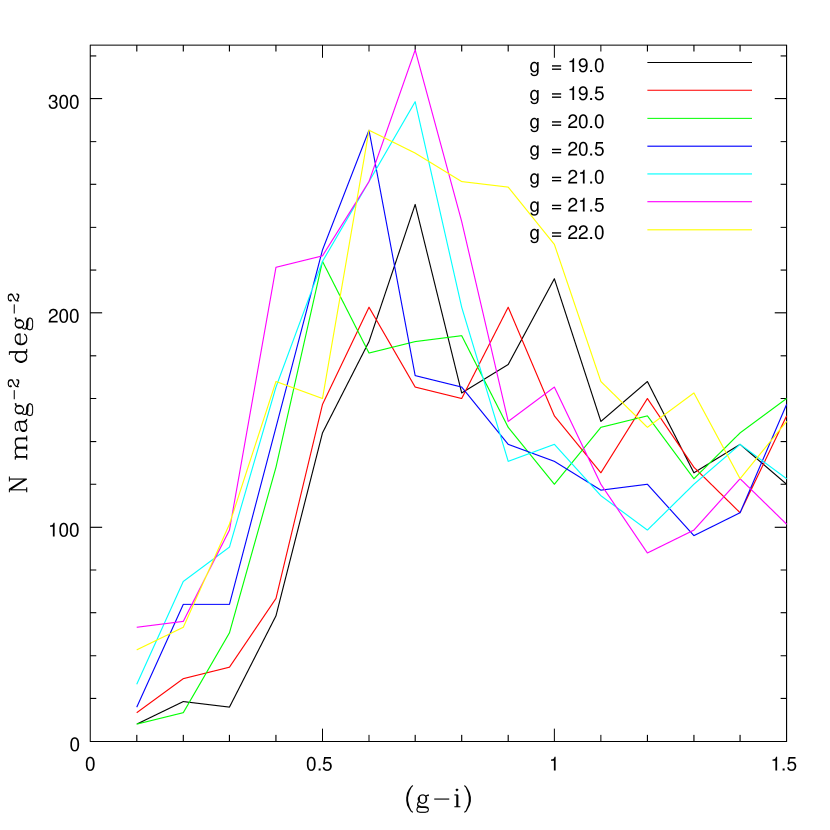
Figure 1: Density ($\rm mag^{-2}\,deg^{-2}$) of stars in the color magnitude diagram of the SDSS high-latitude anti-center field toward $(l,b)=(196,-40)$. Curves correspond to constant-magnitude bins at half-magnitude intervals from $g=19$ to $g=22$. To a first approximation, all the curves are the same. Moreover, they are roughly flat redward of the turnoff (at $g-i\sim 0.65$) and even on the turnoff they are only about double the plateau value.

Because the selection criteria for HVS candidates can only be color and apparent magnitude, we must begin by analyzing the background in terms of these two variables. We adopt a purely empirical approach, tabulating the density of stars toward a SDSS field centered at approximately RA=4 hr , Dec=$-6^{\circ}$ ($l=196$, $b=-40$). Figure 1 shows the stellar density as a function of $g-i$ color for 7 different magnitude bins centered on $g=19.0,19.5.,\ldots 22.0$. The key point is that in this magnitude range and in the region from the turnoff redward, this density varies by less than a factor 4 altogether and only by a factor 2 in the basic trend with color. Moreover the color profiles at each $g$ magnitude are approximately the same. These characteristics imply that the background does not play a crucial role in devising selection procedures for HVS candidates as it would have were the curves clearly separated: rather color/magnitude selection must be based primarily on maximizing the total number of HVSs and minimizing the amount of observing time required to identify them as HVSs. We return to the issue of turnoff vs. giant and lower MS stars in § 2.4.

2.4 Color Selection

Under certain simplifying assumptions, the color/magnitude selection actually factors into separate selections in color and magnitude. We first introduce and motivate these assumptions and later evaluate how their relaxation would impact our conclusions.

First, we assume that deceleration is negligible so that, as mentioned in § 2.1, $\rho\propto R^{-2}$. In fact, for an isothermal sphere of circular velocity $v_{\rm circ}=220\,\,{\rm km\,s}^{-1}$, the velocity-squared falls by $\Delta v^{2}=2v_{\rm circ}^{2}\ln(R_{2}/R_{1})$ between $R_{1}$ and $R_{2}$. For example, a star traveling at $800\,\,{\rm km\,s}^{-1}$ at $15\,\,{\rm kpc}$ will slow by 15% to $675\,\,{\rm km\,s}^{-1}$ at $100\,\,{\rm kpc}$. This is not completely negligible but it is modest compared to other factors in the problem. Under this assumption, the number of HVSs of a fixed absolute magnitude (and so by assumption fixed color) and a narrow range of apparent magnitudes $\Delta g$, is

$$N={\ln 10\over 5}\,{\Gamma\langle v^{-1}\rangle\over 4\pi}\,\Omega\Delta g{r^{3}\over R^{2}}$$ (2)

where $\Omega$ is the angular size of the field and $r$ is the distance from the observer to a star at the center of the magnitude bin.

Second, we assume that $R=r$, which reduces the last term in equation (2) from $r^{3}/R^{2}\rightarrow r$. That is, $N_{\rm naive}\propto r$. The ratio of this naive estimate to the true number is

$${N_{\rm naive}\over N}=1-2\cos l\cos b{R_{0}\over r}+{R_{0}^{2}\over r^{2}}\rightarrow 1+1.47{R_{0}\over r}+{R_{0}^{2}\over r^{2}},$$ (3)

where $R_{0}=8\,\,{\rm kpc}$ is the solar Galactocentric radius. Clearly this correction can be fairly large, so we will have to carefully assess its impact after the selection criteria are derived.

Because radial velocity (RV) measurements are most efficiently carried out in the $g$-band part of the spectrum, RV precision for a fixed exposure time is basically a function of $g$ magnitude. This is not exactly true because the metal lines, from which these determinations are primarily derived for FGK stars, are stronger at lower temperatures. However, this is a modest correction, which we will ignore for the moment but to which we will return below.

Consider now an ensemble of HVSs, drawn randomly from a common old-star isochrone and ejected isotropically and stochastically from the Galactic center. We now select stars at a fixed $g$-magnitude (or rather in a narrow interval $\Delta g$ centered at fixed $g$), which have a variety of absolute magnitudes $M_{g}$ and so (through the color-magnitude relation of the isochrone), a variety of $g-i$ colors (which are what we actually observe). The stars at $M_{g}$ will be seen over a range of distance $\Delta r=(\ln 10/5)10^{0.2(g-M_{g}+5)}\Delta g\,$pc, i.e. $\Delta r\propto 10^{-0.2\,M_{g}}$. Under the above two assumptions, the relative number of such stars in the sample will be

$$N_{det}(M_{g})\propto 10^{-0.2\,M_{g}}\Phi(M_{g}),$$ (4)

where $\Phi(M_{g})$ is the fraction of stars from the isochrone in the $M_{g}$ bin. Note, in particular that this relative number does not depend on $g$, the apparent magnitude at which they are selected.

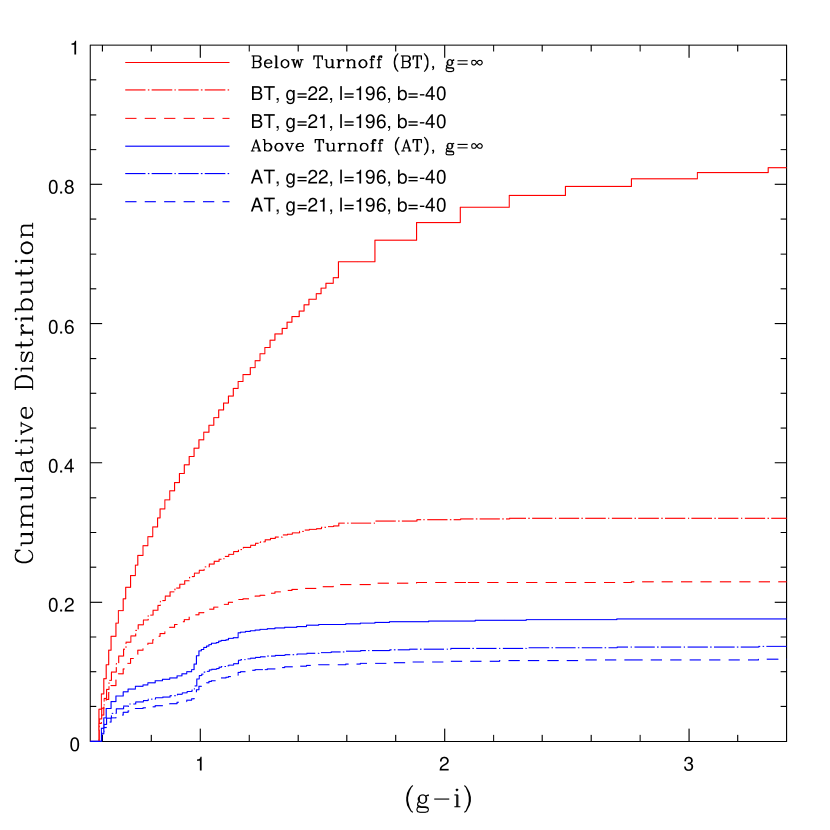
Figure 2: Cumulative distribution of expected high-velocity-star detections of apparent magnitude $g$ as a function of $g-i$ color, under the assumption that all stars in the underlying old-population are equally likely to be ejected from the Galactic center. The red curves represent stars below the main-sequence turnoff while the blue curves represent stars above the turnoff. At very faint magnitudes, the result is independent of magnitude and is shown by the two solid curves, whose total is arbitrarily normalized to unity. At realistic magnitudes, $g=22$ (dot-dashed) or $g=21$ (dashed), the detections are somewhat suppressed by eq. (3), particularly for the below-turnoff branch. For these curves, the great majority of expected detections are at $g-i<1.1$.

Figure 2 shows the cumulative distribution of these relative numbers as a function of color (the observed quantity) for an isochrone of solar metallicity and age of 10 Gyr (Demarque et al., 2004). Since these are given in the Johnson/Cousins system, we convert to SDSS bands using the transformations given on the SDSS web site (Lupton, 2005). When the isochrone is viewed as a “function” of color, it is double-valued. To illustrate the role of the two branches, we plot their cumulative distributions separately, although of course these could not be distinguished from color/magnitude data alone. The solid curves illustrate the result under the assumption that $r=R$, i.e., effectively that $g=\infty$. The dashed and dot-dashed curves are for the more realistic cases of $g=22$ and $g=21$ in the direction $(l,b)=(196^{\circ},-40^{\circ})$.

There are several important features of this diagram. First, and by far the most important, the great majority of potential sensitivity to old-population HVSs comes from stars with $g-i$ colors within 0.5 magnitudes of the turnoff, i.e., with $g-i<1.1$. This is already basically true for the naive “$g=\infty$” case, but strictly applies in realistic cases, $g\lesssim 22$. By contrast, both the M and late-K dwarfs on the lower branch and the M and late-K giants on the upper branch, contribute very little, the former because they are so close and the latter because they are so rare. Note that the dominance of turnoff stars is a specific result of the $L^{1/2}$ luminosity-dependence in equation (4). If $N\propto L^{3/2}$ (as in a magnitude-limited sample of uniform-density population) then giants would dominate. If $N\propto L^{0}$ (as in a magnitude-limited sample of an $r^{-3}$ halo-star-like population) then dwarfs would dominate. Second, the lower branch contributes a bit more than double the upper branch for realistic cases. That is, the sample is dominated by stars just below the turnoff, with a significant, though clearly secondary, contribution from stars just above the turnoff. This implies that the validity of our approximations is basically determined by how well they hold up at the turnoff. Third, the small contribution from late-type giants obviates another potential complication. Depending on the precise form of the ejection mechanisms, it is possible that giant-star ejection is suppressed relative to smaller stars. For example, some or all of the ejections might take place from disruption of relatively tight binaries that are too close to permit giant-star survival. Had Figure 2 implied giants dominated the HVS distribution, this would lead to significant uncertainty. However, the small contribution of giants, particularly late-type giants, implies that any such suppression would also have small impact. The one exception to this is the clump giants, which are not included in the Yale Isochrones and hence are not represented in this figure. They would contribute a small “bump” in the “above turnoff” curve, similar in amplitude to the bump at $g-i\sim 1$ that is actually seen in this curve, which is due to first-ascent giants. With radii ten times solar, these stars are themselves relatively small. However, with ages of only $100\,$Myr, they are younger than the transport time to their current location, roughly $200\,$Myr at $g=21$ and velocity $v=700\,\,{\rm km\,s}^{-1}$. Hence, the progenitors of these stars would have had to have been ejected when they were very distended. In any event, they are not included in the figure. Finally, the slightly greater RV precision (at fixed $g$ and fixed exposure time) of cooler stars also has negligible impact, again because of the small contribution of these stars.

From this analysis, we conclude that at fixed magnitude, selection should stretch from the turnoff and proceed redward to $g-i=1.1$. In practice, the old-population HVSs will not come from a single isochrone, but from a superposition of many isochrones with a variety of ages and metallicities. However, all of these are qualitatively similar, with just slightly varying turnoff colors. Indeed, we investigated a 5 Gyr isochrone and found results qualitatively similar to those shown in Figure 2. The important practical point is just to sample the field stars beginning blue enough to cover all such turnoffs. The cost of moving the blue boundary further blueward by $\Delta(g-i)=0.3$ is quite small, since this region of the observed field-star color-magnitude diagram has few stars. We therefore advocate color selection $0.3<g-i<1.1$.

2.5 Magnitude Selection

Observations of a fixed exposure time can potentially measure RVs to a given precision down to a certain apparent-magnitude limit $g$. Once this is established, one could in principle measure RVs for all stars within this limit, or (if fibers/slits were scarce) only those within 2 magnitudes of the limit, which would contain $>60\%$ of all the HVSs within the magnitude limit. The following arguments apply equally to either strategy.

Let us first suppose that “downtime” (for slewing, readout, and changing slit masks or fiber positions) is negligible compared to the exposure time. Let us compare two observation strategies, the first with a single field exposed for time $\Delta t$ and the second with two fields each exposed for $\Delta t/2$. Let us initially assume that the magnitude limit is above sky in both cases. Then the flux limit will be a factor 2 larger in the second case to maintain the same signal-to-noise ratio (S/N). The maximum observable distance will therefore be reduced by $2^{-1/2}$, which will decrease the number of HVSs detected in each field by the same factor. However, since there are twice as many fields, the total number of detected HVSs will increase by $2^{1/2}$. Hence it is always better to go to shorter exposures of more fields. If both limits are below sky, then the flux limit increases by $2^{1/2}$, so the distance limit decreases by $2^{-1/4}$, and the number of HVSs from both fields increases by $2^{3/4}$. That is, the same argument applies even more strongly.

Now consider the opposite limit, in which the exposure time is negligible compared to the downtime. Shortening the exposure time then still increases the flux limit and so reduces the number of HVSs detected by $2^{-1/2}$ but in this case there is no compensating increase in the number of fields covered. Comparing the two cases, it is clear that the exposure times should be set approximately equal to the downtime. It can be shown that the optimal exposure time is exactly equal to the downtime if the magnitude limit is above sky and equal to 1/3 of the downtime if it is below the sky.

This argument somewhat overstates the case: it would be strictly valid if the cumulative distributions illustrated in Figure 2 were identical for the limiting magnitudes corresponding to the two different exposure times. These curves are nearly identical for the upper branch, but less so for the lower branch. However, the argument remains qualitatively valid, the correction being toward exposures that are somewhat longer than the downtime.

2.6 Observing Strategy: General Considerations

Before analyzing the characteristics of specific spectrographs, there are two general points to consider. First, from Figure 1, the stellar density in our recommended color range, $0.3<g-i<1.1$, is about $150\,\rm mag^{-1}\,deg^{-2}$. Hence, if one is to cover 2 or 3 magnitudes in $g$, this requires monitoring 300–500 stars per square degree. Note that in another direction, $(l,b)=(275^{\circ},62^{\circ})$, we find stellar densities in this color-mag range that are about 2.5 times higher, confirming that it is substantially easier (in terms of the sheer number of background contaminants) to search for old-population HVS in high-latitude anticenter fields.

Second, the RV precision requirements to distinguish HVSs from halo stars are not very severe: $\sigma=50\,\,{\rm km\,s}^{-1}$ would be quite adequate. Typical HVSs have RVs $v_{r}\sim 700\,\,{\rm km\,s}^{-1}$, well separated from halo stars at $|v_{r}|\sim O(170\,\,{\rm km\,s}^{-1})$. There are, of course, halo stars moving closer to the escape velocity, but these are relatively rare, and the chance that one of these would further upscatter by $\sim 5\,\sigma$ into the HVS range is quite small. This precision is not difficult to achieve even in very noisy spectra, particularly on FGK stars, which have many spectral features.

2.7 Specific Evaluations

From this point forward, concrete development of an observing strategy obviously depends on the detailed characteristics of the multi-object spectrograph, which cannot be treated completely generally. However, to give some broad guidance and to help understand the sensitivity of the search under realistic conditions, we consider two specific multi-object spectrographs with radically different characteristics.

First, we consider the resolution ${\cal R}=2000$ SDSS spectrograph, which has 640 $3^{\prime\prime}$ diameter fibers spanning a $7\,\rm deg^{2}$ field on a 2.5 m telescope. The fiber plug-plates require about 10 minutes to change. In principle, one should consider the time required for repointing the telescope, but this will be relatively infrequent because even in the anticenter fields, there are about 2000 viable targets (for a 2-magnitude interval) and only 640 fibers, so there should be about three plug-plates per pointing. If we strictly applied the “exposure time equals downtime” rule, the resulting 10 minute exposure would yield per pixel S/N=10 at about $g=19.5$. Given the $3^{\prime\prime}$ fibers, this is about 1 mag below dark sky. In practice, it is probably impractical to change plug plates so frequently, so 45 minute exposures (in keeping with current SDSS practice) would appear more realistic. Taking account of sky, this yields a per pixel S/N=8 at $g=20.5$ and S/N=4 at $g=21.5$. This latter is probably adequate for $\sigma=50\,\,{\rm km\,s}^{-1}$ measurements, but this should be tested directly. Hence, in one 9-hour night, the SDSS telescope could cover a total of $21\,\rm deg^{2}$ over $19.5<g<21.5$ and $0.3<g-i<1.1$, i.e., 3 45-minute exposures (1 for each of 3 plug plates) on each of 3 fields. One additional wrinkle should be noted. The 640 fibers are divided into 320 red and 320 blue channels, with the dividing line at 6000 Å. The blue-channel fibers are more sensitive to RV because of the greater density of lines. However, this can easily be compensated by applying the red-channel fibers to the brighter stars. Being systematically 1 magnitude brighter (and recalling that the target stars are mostly below sky), these would have about 2.5 times higher S/N per pixel.

Second, we consider the ${\cal R}=20000$ IMACS F/4 spectrograph, which accommodates up to 1000 slits spanning a $0.067\,\rm deg^{2}$ field on the Magellan 6.5 m telescope. Changing slit masks requires about 15 minutes, but in fact this is not the relevant scale of “downtime” because each field has only of order 20–30 available targets, far fewer than the available slits. Rather, each mask could be cut to serve of order 10 fields (with a total of 200-300 targets). Hence, the downtime is primarily set by the time required to acquire a new field (without changing the mask). This is roughly 5 minutes, which by the guideline derived in § 2.5 would indicate an exposure time also of 5 minutes. Taking account of sky noise and assuming $4\,e^{-}$ read noise, this leads to an estimate of per pixel S/N=1.2 at $g=21.5$. To evaluate the utility of such signal levels, we construct synthetic spectra, add noise, and then fit the results to a (4-parameter) quadratic polynomial plus a template spectrum, offset by various velocities from the constructed spectrum. We find that this S/N is sufficient for an accurate RV measurement, provided that at least $80\,$Å are sampled centered on $\lambda=5175\,$Å. In fact, the formal error in the measurement is less than $10\,\,{\rm km\,s}^{-1}$, so that it would appear that even lower S/N would be tolerable. However, we find if the S/N is further reduced, that while the width of the correlation peak does not increase dramatically, multiple minima (each quite narrow) begin to appear, undermining the measurement. Similarly, if the wavelength coverage is reduced at constant S/N, then multiple minima also appear. In any event, if appropriate blocking filters permit this $80\,$Å (800 pixel) window or larger, then the field can be reliably probed to $g=21.5$. Of order 50 fields could be searched during a 9 hour night, covering about $3.3\,\rm deg^{2}$.

Thus, while these two spectrographs differ in aperture, resolution, and field size by factors of 7, 10, and 100 respectively, they are capable of broadly similar searches for HVSs. We conclude that it is feasible to conduct the search over tens of square degrees on a variety of telescopes without exorbitant effort.

3 Discussion

How likely is it that such a survey of several tens of square degrees will detect old-population HVSs? At one level, as emphasized in § 1, we have no idea: based on what we know now, old-population HVSs could equally well be very common or non-existent. However, in the absence of any hard information, we might guess that the ratio of old-population to B-type HVSs might be similar to the ratio of the underlying populations near the GC. This itself is not known, but as proxy we evaluate the same ratio in the solar neighborhood. In fact, what is required is the ratio of turnoff stars to B stars, since our proposed survey is most sensitive to turnoff stars, while B stars form the only population of HVSs that have been reliably tabulated. The distance ranges are similar: the B stars have typically been detected at 60 kpc while turnoff stars at $g=21.5$ lie at about 25 kpc (a factor 2.5 advantage for the B stars) but the B stars were searched over 1 mag in $g$ while the turnoff stars would be searched over 2 mags (which basically compensates).

We estimate the ratio of $B$ stars to turnoff stars in the solar neighborhood as follows. We analyze samples of each stellar class drawn from the Hipparcos catalog (ESA, 1997), restricted to $V<7.3$ (Hipparcos completeness limit), distance $r<300\,$pc (to ensure good parallaxes and low extinction), and distance from the Galactic plane less than 50 pc. We define turnoff stars as having absolute magnitudes $3.5<M_{V}<4.5$ and near-turnoff colors ($0.3<B_{T}-V_{T}<0.8$). For B stars, we probe a 2-magnitude interval $-2.0<M_{V}<0.0$, which approximately corresponds to the Brown et al. (2006) $g-r$ selection criterion, and we enforce ($-0.5<B_{T}-V_{T}<0.2$) to distinguish these from giants. For each class of star, we tabulate $\sum_{i}(V_{{\rm eff},i})^{-1}$, where $V_{{\rm eff},i}$ is the “effective volume” over which that star could have been found. That is $V_{{\rm eff}}=4\pi r_{\rm max}^{3}$ where $r_{\rm max}$ is the maximum distance that star could have been detected given its observed absolute magnitude, its known direction, and the two constraints on distance given above. We find effective densities of $0.91\times 10^{-5}\,\rm pc^{-3}$ and $60.7\times 10^{-5}\,\rm pc^{-3}$ for the two classes, indicating that turnoff stars are about 67 times more common that B stars.

Applying this rather crudely derived multiplier to the B-star HVS density found by Brown et al. (2006), we estimate that there could be 1 turnoff HVS per $10\,\rm deg^{2}$. Hence a survey of a few tens of square degrees could probe the existence of this putative population.

References

- Baumgardt et al. (2006) Baumgardt, H., Gualandris, A., & Portegies Zwart, S. 2006, Journal of Physics Conference Series, 54, 301
- Brown et al. (2005) Brown, W. R., Geller, M. J., Kenyon, S. J., & Kurtz, M. J. 2005, ApJ, 622, L33
- Brown et al. (2006) Brown, W.,R. et al. 2006, astro-ph/0604111
- ESA (1997) European Space Agency (ESA). 1997, The Hipparcos and Tycho Catalogues (SP-1200; Noordwijk: ESA)
- Edelmann et al. (2005) Edelmann, H., Napiwotzki, R., Heber, U., Christlieb, N., & Reimers, D. 2005, ApJ, 634, L181
- Fuentes et al. (2006) Fuentes, C. I., Stanek, K. Z., Gaudi, B. S., McLeod, B. A., Bogdanov, S., Hartman, J. D., Hickox, R. C., & Holman, M. J. 2006, ApJ, 636, L37
- Gould et al. (1998) Gould, A., Flynn, C., & Bahcall, J.N. 1998, ApJ, 503, 798
- Gnedin et al. (2005) Gnedin, O. Y., Gould, A., Miralda-Escudé, J., & Zentner, A. R. 2005, ApJ, 634, 344
- Hansen & Milosavljević (2003) Hansen, B. M. S., & Milosavljević, M. 2003, ApJ, 593, L77
- Hills (1988) Hills, J. G. 1988, Nature, 331, 687
- Hirsch et al. (2005) Hirsch, H. A., Heber, U., O’Toole, S. J., & Bresolin, F. 2005, A&A, 444, L61
- Lupton (2005) Lupton, R. 2005, http://www.sdss.org/dr5/algorithms/sdssUBVRITransform.html.
- Demarque et al. (2004) Demarque, P., Woo, ¿ J.-H., Kim, Y.-C., & Yi, S.K. 2004, ApJS, 155, 667
- Yu & Tremaine (2003) Yu, Q., & Tremaine, S. 2003, ApJ, 599, 1129