The depletion of NO in pre–protostellar cores

Abstract

Context. Understanding the depletion of heavy elements is a fundamental step towards determining the structure of pre–protostellar cores just prior to collapse.

Aims. We study the dependence of the NO abundance on position in the pre–protostellar cores L1544 and L183.

Methods. We observed the 150 GHz and 250 GHz transitions of NO and the 93 GHz transitions of N₂H⁺ towards L1544 and L183 using the IRAM 30 m telescope. We compare the variation of the NO column density with position in these objects with the H column density derived from dust emission measurements.

Results. We find that NO behaves differently from N₂H⁺ and appears to be partially depleted in the high density core of L1544. Other oxygen–containing compounds are also likely to be partially depleted in dense–core nuclei. The principal conclusions are that: the prestellar core L1544 is likely to be ‘carbon–rich’; the nitrogen chemistry did not reach equilibrium prior to gravitational collapse, and nitrogen is initially (at densities of the order of $10^{4}$ cm^-3) mainly in atomic form; the grain sticking probabilities of atomic C, N and, probably, O are significantly smaller than unity.

Conclusions.

1 Introduction

It is now accepted that most, if not all, C–containing species deplete on to dust grain surfaces in the central, high–density regions of prestellar cores. Thus, when one compares a map of C¹⁸O, for example, with that of the dust emission, one sees that the CO isotopomer traces only an outer shell and not the high–density interior ($n_{\rm H}\mathrel{\hbox{\hbox to0.0pt{\hbox{\lower 4.0pt\hbox{$\sim$}}\hss}\hbox{$>$}}}3\times 10^{4}$ cm^-3); this limits our understanding of prestellar cores, because the molecular line emission provides information on the kinematics.

Surprisingly, N–containing species (in particular, NH₃ and N₂H⁺) manage to remain in the gas phase up to densities of a few times $10^{5}$ cm^-3. It is not entirely clear what happens at still higher densities, but it seems likely that the N–containing species disappear from the gas phase when $n_{\rm H}\mathrel{\hbox{\hbox to0.0pt{\hbox{\lower 4.0pt\hbox{$\sim$}}\hss}\hbox{$>$}}}10^{6}$ cm^-3 (see, for example, Belloche & André 2004, Pagani et al. 2005). The different behaviour of the N–containing species was originally attributed to the relatively high volatility of N₂ on grain surfaces (Bergin & Langer (1997), Aikawa et al. (2001)), but recent laboratory measurements (Öberg et al. (2005), Bisschop et al. (2006)) show that N₂ is only marginally more volatile than CO. This result throws doubt on much recent modelling of the chemistry of prestellar cores and poses the question of whether another more volatile and abundant form of nitrogen is responsible for the survival of N–containing species to high density. Another possibility is that atomic nitrogen does not stick effectively to grain surfaces. In recent studies (Flower et al. 2005, 2006), we have explored this suggestion and found that the best fit of the models to the observed abundances of NH₃ and N₂H⁺ is obtained when the sticking probabilities of both atomic N and O are low and, additionally, the mean grain surface area per H atom is a factor 5–10 lower than in the diffuse interstellar medium; this implies that considerable grain growth has occurred prior to the prestellar–core phase.

In all of this discussion, the abundance of oxygen–containing species, such as OH and water, has been somewhat neglected, and for good reason. OH and water are hard to observe with reasonable (arc min or better) resolution in cold clouds (see, for example, Goldsmith & Li 2005, Bergin & Snell 2002). Thus we do not presently know whether oxygen–containing species survive in the gas phase in the regions where N₂H⁺  and NH₃ are observed. In the long run, observations of water with the HIFI instrument on the Herschel satellite or of OH with the Square Kilometer Array (SKA) may provide an answer. In the meantime, we need to consider alternative observational strategies, using chemical models of prestellar cores as a guide. If atomic oxygen sticks to grain surfaces no more efficiently than atomic nitrogen, OH and H₂O  might be expected to survive in the gas phase similarly to NH₃ and N₂H⁺.

An important aspect of this problem involves NO, which is believed to be a key molecule in the nitrogen chemistry. NO mediates the transformation of atomic into molecular nitrogen, in the reactions

$${\rm N}+{\rm OH}\rightarrow{\rm H}+{\rm NO}$$ (1)

and

$${\rm N}+{\rm NO}\rightarrow{\rm O}+{\rm N}_{2}$$ (2)

Atomic and molecular nitrogen are expected to be the major forms of elemental nitrogen in the gas phase. Under conditions in which reactions (1) and (2) dominate the formation and destruction, respectively, of NO, the ratio of the abundance of NO to that of OH is given simply by the ratio of the rate coefficients for these reactions, $k_{1}/k_{2}$; $k_{1}/k_{2}\approx 1$, providing that there are no energy barriers to these reactions, which might reduce differentially the values of their rate coefficients at low temperatures. Then, one might consider NO to be a proxy for OH, providing information on O–containing species in the gas phase. OH forms through a sequence of reactions which is initiated by O(H${}_{3}^{+}$, H₂)OH⁺ (and the analogous reactions with the deuterated isotopes, H₂D⁺ and D₂H⁺), followed by hydrogenation by H₂ and dissociative recombination with electrons. OH is destroyed principally in the reactions O(OH, O₂)H and N(OH, NO)H. Thus, the abundance of OH is tied to the abundances of H${}_{3}^{+}$, H₂D⁺ and D₂H⁺, and OH is a minor oxygen–containing species.

NO is a known interstellar molecule, which has been detected in L183 with a fractional abundance of around $10^{-7}$ (see Gerin et al. 1992, 1993). The value quoted by these authors was an overestimate, as it was based on the C¹⁸O column density, and CO is now known to be depleted in L183 (Pagani et al. 2004, 2005). Nonetheless, the fractional abundance of NO is high, which encouraged us to investigate the spatial variation of the NO abundance in the cores L183 and L1544. For these objects, estimates of the column densities of molecular hydrogen, $N$(H₂), which are independent of the degree of depletion, may be made from the existing maps of the dust emission. Our objective was to compare the spatial variations of the NO and H₂ (from the dust) column densities. In addition, we observed simultaneously with NO the $J=1\rightarrow 0$ transitions of N₂H⁺, which are known to follow roughly the dust emission.

In Sect. 2, we describe our observations and, in Sect. 3, give the observational results. Comparisons with model predictions are made in Sect. 4, and our concluding remarks are to be found in Sect. 5.

2 Observations

The observations were carried out during two sessions, in July and August 2005, using the IRAM 30 m telescope. We observed simultaneously with the facility 3 mm, 2 mm, and 1.3 mm receivers. The 3 mm receiver was tuned to the N₂H⁺ $J=1\rightarrow 0$ 93.17632 GHz line, the 2 mm receiver to the centre of the NO $J=3/2\rightarrow 1/2$ $\Pi^{+}$ and $\Pi^{-}$ transitions at 150.36146 GHz, and the 1.3 mm receiver to the centre of the NO $J=5/2\rightarrow 3/2$ $\Pi^{+}$ and $\Pi^{-}$ transitions at 250.61664 GHz. The half–power beam widths at these three frequencies are 27${}^{{}^{\prime\prime}}$, 16${}^{{}^{\prime\prime}}$, and 10${}^{{}^{\prime\prime}}$, respectively, and the corresponding main–beam efficiencies are 0.78, 0.68, and 0.48. Pointing was checked at intervals of roughly 2 hours and was found to be accurate within 2${}^{{}^{\prime\prime}}$. We used central positions (J2000) of R.A. = $05^{\rm h}04^{\rm m}16^{\rm s}.9$, Dec. = 25${}^{\circ}10^{{}^{\prime}}47^{{}^{\prime\prime}}.7$ for L1544 and R.A. = $15^{\rm h}54^{\rm m}08^{\rm s}.8$, Dec. = $-02^{\circ}52^{{}^{\prime}}44^{{}^{\prime\prime}}.0$ for L183, and the offsets specified below are with respect to these positions.

We used the facility SIS receivers in frequency–switching mode with system temperatures of 150–180 K at 3 mm, 350–450 K at 2 mm, and 1000–2000 K at 1.3 mm. At 3 mm, we used the facility VESPA autocorrelator as a spectral backend with 20 kHz channel spacing over a 20 MHz band, allowing us to cover all 7 hyperfine satellites of the N₂H⁺($J=1\rightarrow 0$) transition. At 2 mm and at 1.3 mm, the NO lines are too widely separated to be covered in one band with adequate resolution. We therefore split VESPA into 6 parts of 20 MHz bandwidth and 20 kHz resolution at 2 mm and 3 parts with 40 MHz bandwidth and 40 kHz resolution at 1.3 mm. The different sections of the autocorrelator were offset so as to cover the frequencies and transitions summarized in Table 1. The corresponding velocity resolutions were 0.04 km s^-1 at 2 mm and 0.05 km s^-1 at 1.3 mm. The data were processed using the GILDAS package.

Table 1: NO line parameters

Transition	Frequency	Line Strength1
$J^{{}^{\prime}},F^{{}^{\prime}}\rightarrow J^{{}^{\prime\prime}},F^{{}^{\prime\prime}}$	GHz
$\Pi^{+}$
$\frac{3}{2},\frac{5}{2}\rightarrow\frac{1}{2},\frac{3}{2}$	150.17646	0.500
$\frac{3}{2},\frac{3}{2}\rightarrow\frac{1}{2},\frac{1}{2}$	150.19876	0.186
$\frac{3}{2},\frac{3}{2}\rightarrow\frac{1}{2},\frac{3}{2}$	150.21874	0.148
$\frac{3}{2},\frac{1}{2}\rightarrow\frac{1}{2},\frac{1}{2}$	150.22565	0.148
$\Pi^{-}$
$\frac{3}{2},\frac{5}{2}\rightarrow\frac{1}{2},\frac{3}{2}$	150.54646	0.500
$\frac{3}{2},\frac{1}{2}\rightarrow\frac{1}{2},\frac{1}{2}$	150.58055	0.148
$\Pi^{+}$
$\frac{5}{2},\frac{7}{2}\rightarrow\frac{3}{2},\frac{5}{2}$	250.43684	0.445
$\Pi^{-}$
$\frac{5}{2},\frac{7}{2}\rightarrow\frac{3}{2},\frac{5}{2}$	250.79643	0.445
$\frac{5}{2},\frac{5}{2}\rightarrow\frac{3}{2},\frac{3}{2}$	250.81561	0.280
(1) Gerin et al. (1992)

3 Results

In Appendix A, we describe the method used to determine the column densities of N₂H⁺, which are used in the chemical analysis presented in the following Section. Here, we discuss the derivation of the column densities of NO for each of the two prestellar cores which we observed.

3.1 L1544

In the time available, rather than attempting to map the NO emission, we observed along two cuts, in the NW–SE and NE–SW directions, centred on the origin given in Sect. 2; these directions correspond roughly to the major and minor axes, respectively, of the dust emission, which we assume to be a good representation of the total column density distribution. Furthermore, the intensities of the NO 150 GHz (2 mm) lines are expected to yield a good approximation to the true NO column density distribution (see Gerin et al. (1992)), as long as the lines are optically thin; this is likely to be the case, given their relative weakness (the low $J$ levels are expected to be thermalized in L1544). Furthermore, the relative intensities of the different hyperfine components are observed to be close to the values expected on the basis of the line strengths in Table 1. Averaging the corresponding transitions from the $\Pi^{+}$ and $\Pi^{-}$ bands, we find a ratio of $0.46\pm 0.07$ between the $J=3/2\rightarrow 1/2$ $F=3/2\rightarrow 1/2$ and $F=5/2\rightarrow 3/2$ lines (at zero offset, (0,0): see Table 2), as compared to 0.37 using the line strengths in Table 1. Similarly, the ratio of the average of the three 2 mm lines with strength 0.148 in Table 1 to the two lines with strength 0.500 is measured to be $0.30\pm 0.04$, as compared with 0.30 in the optically thin LTE limit. Thus, we find that the NO hyperfine satellite intensities are almost consistent, to within the error bars, with the low optical depth limit. We can then convert the integrated intensity $I$(2 mm) in the $J=3/2\rightarrow 1/2$ $F=5/2\rightarrow 3/2$ (average of $\Pi^{+}$ and $\Pi^{-}$) into an NO column density for a given excitation temperature, $T_{\rm{ex}}$(NO).

Table 2: NO transitions observed towards L1544 (0,0), with uncertainties in parentheses. The linewidths of the 150 GHz transitions were determined by means of a gaussian fit, using the CLASS procedure; the linewidths of the (noisier) 250 GHz lines were fixed to that of the 150.17646 GHz transition.

Frequency	Integrated intensity	$V_{\rm{lsr}}$	$\Delta v$
GHz	K km s-1	km s-1	km s-1
150.17646	0.22(0.02)	7.18(0.01)	0.38(0.02)
150.19876	0.09(0.01)	7.14(0.02)	0.35(0.04)
150.21874	0.05(0.01)	7.12(0.02)	0.30(0.04)
150.22565	0.06(0.01)	7.12(0.02)	0.26(0.04)
150.54646	0.20(0.01)	7.11(0.01)	0.34(0.02)
150.58055	0.04(0.01)	7.13(0.03)	0.34(0.06)
250.43684	0.26(0.04)	7.28(0.05)	0.38
250.79643	0.22(0.04)	7.26(0.04)	0.38

Because NO has a small dipole moment, the critical density (at which the rates of collisional and radiative de-excitation are equal) is of order $10^{4}$ cm^-3, and it seems reasonable to suppose thermalization of the NO levels of interest to us here. Based on the NH₃ results of Tafalla et al. (2002), we assume $T_{\rm{ex}}=8.75$ K and find that the column density of NO cm^-2 in L1544 should be given approximately by

$$N({\rm NO})=4.3\times 10^{15}\,I(2\,{\rm mm})$$

where $I$(2 mm) K km s^-1 denotes the intensity of the NO 2 mm (150 GHz) lines (see Gerin et al. (1992), table 3). We note that new VLA observations by Crapsi et al. (2005b) suggest that the temperature decreases towards the dust peak; but, as we shall see below, NO is likely to be depleted at high densities, and so we use the single–dish temperature estimate. An independent check of the NO excitation is provided by our measurements of the $J=5/2\rightarrow 3/2$ 250 GHz lines. From Table 2, we conclude that $I$(1.2 mm)/$I$(2 mm) = $1.14\pm 0.25$, where, in addition to the formal errors given in the Table, we have assumed a 15 percent calibration error. Here, $I$(1.2 mm) is the average of the integrated intensities of the two $J=5/2\rightarrow 3/2$ $F=7/2\rightarrow 5/2$ transitions. Using the formulation of Gerin et al. (1992), we find that the corresponding excitation temperature between the $J=5/2$ and $J=3/2$ levels is $T_{\rm{ex}}=13.5\pm 4$ K, which is higher than the single–dish NH₃ measurement but consistent with it, to within the combined error bars.

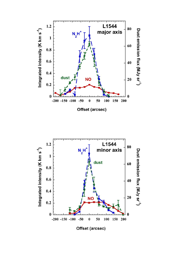
Figure 1: Plots of the average of the integrated intensities of the NO $\Pi^{+}$ and $\Pi^{-}$ $J,F=3/2,5/2\rightarrow J,F=1/2,3/2$ lines (see Table 1), denoted by full curve joining circles with error bars, which have approximately the same size as the symbols, plotted against offset from the (0,0) position in L1544. Increasing offset is in the sense of increasing R.A. The top panel shows the cut along the NE–SW major axis, and the bottom panel the cut along the NW–SE minor axis. We show also for comparison the integrated intensity of the 93.17632 GHz transition of N₂H⁺ (squares joined by long broken curve) and the 1.2 mm dust emission (diamonds joined by short broken curve), from Ward-Thompson et al. (1999). The error bars plotted correspond to RMS deviations from the fits (gaussian for the lines); thus we neglect systematic errors arising from the calibration, for example. The NO measurements involved long integration times, and the two components ($\Pi^{+}$ and $\Pi^{-}$) were averaged, whence the small error bars in this case. The intensities derive from main–beam brightness temperatures.

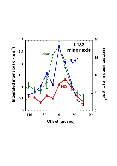
Figure 2: Plots of the average of the integrated intensities of the NO $\Pi^{+}$ and $\Pi^{-}$ $J,F=3/2,5/2\rightarrow J,F=1/2,3/2$ lines (see Table 1), denoted by full curve joining circles with error bars, against offset from the (0,0) position in L183. Increasing offset is in the sense of increasing R.A. The cut is along the E–W (minor) axis. We show also for comparison the integrated intensity of the 93.17632 GHz transition of N₂H⁺ (squares joined by long broken curve) and the 1.2 mm dust emission (diamonds joined by short broken curve), from Pagani et al. (2004). The intensities derive from main–beam brightness temperatures.

In Fig. 1, we show our observations of NO at 2 mm for both the NE–SW and NW–SE cuts, together with the corresponding measurements of the dust emission (from the map of Ward-Thompson et al. (1999)) and our 3 mm observations of N₂H⁺ $J,F_{1},F=1,0,1\rightarrow 0,1,2$ (93.17632 GHz) transition. In essence, these data show that, while the dust and the N₂H⁺ emission peak at the (0,0) position and have an angular size of about 1${}^{{}^{\prime}}$ by 2${}^{{}^{\prime}}$ (0.04 pc by 0.08 pc at the adopted distance of 140 pc of L1544; Crapsi et al. 2005a ), the NO emission extends over at least 3${}^{{}^{\prime}}$ and weakens, relative to the N₂H⁺ and dust emission, towards the (0,0) position. We can quantify this result by using estimates from Fig. 1 of the flux in the dust continuum emission. We derive a peak of emission at 1.2 mm of 225 mJy in the beam, which corresponds, for an assumed dust absorption coefficient $\kappa$ per unit mass density $\rho$ of gas, $\kappa/\rho=0.01$ cm² g^-1, to an H₂ column density of $1.2\times 10^{23}$ cm^-2; we have assumed that the dust temperature is equal to the excitation temperature, $T_{\rm{ex}}=8.75$ K. This conversion factor was used to derive the column density ratio, $x$(NO) = $N$(NO)/$N$(H₂), shown in Fig. 3. We see that the observed column density ratio is approximately $8\times 10^{-9}$ at the dust peak and increases to values of $3\times 10^{-8}$ to $5\times 10^{-8}$ at offsets of around 1${}^{{}^{\prime}}$ (equivalent to 0.04 pc, or 8000 AU) along the minor axis, where the H₂ column density, derived from the dust emission, is a factor of 6 lower than at the peak. Along the major axis, the variation is less marked, but there is also an increase in the column density ratio away from the peak of the dust emission. We suggest in the next Section that this behaviour is probably related to the partial depletion, at high densities, of the main forms of oxygen.

3.2 L183

Our observed line parameters, towards the (0,0) position of L183, are given in Table 3. In this case, only one cut was possible in the time available, in an E–W direction, and the results are shown in Fig. 2.

We have used a procedure to derive the NO abundance similar to that for L1544. We assume a temperature of 9 K, based on the NH₃ results of Ungerechts et al. (1980), in order to compute both the NO and H₂ column densities. We use additionally the dust emission map of Pagani et al. (2004). As discussed below, our NO column density peak in L183 appears to be shifted by about 10${}^{{}^{\prime\prime}}$ in R.A., relative to the dust peak (roughly 1000 AU for an assumed distance of 110 pc; Franco (1989)). We infer column density ratios, $N$(NO)/$N$(H₂), in the range $1\times 10^{-8}$ to $3\times 10^{-8}$, similar to the values derived for L1544.

Table 3: NO transitions observed towards L183 (0,0), with uncertainties in parentheses

Frequency	Integrated intensity	$V_{\rm{lsr}}$	$\Delta v$
GHz	K km s-1	km s-1	km s-1
150.17646	0.47(0.015)	2.37(0.01)	0.38(0.02)
150.19876	0.18(0.015)	2.37(0.02)	0.44(0.04)
150.21874	0.14(0.014)	2.29(0.02)	0.38(0.04)
150.22565	0.14(0.014)	2.35(0.02)	0.32(0.04)
150.54646	0.46(0.016)	2.38(0.01)	0.38(0.02)
150.58055	0.12(0.012)	2.38(0.02)	0.29(0.04)
250.43684	0.27(0.060)	2.33(0.01)	0.11(0.03)
250.79643	0.32(0.060)	2.38(0.02)	0.27(0.06)

4 Modelling the NO abundance distribution

The simple models discussed below are based on the assumption of spherical symmetry, which is clearly a rough approximation for both of the prestellar cores which we consider. Indeed, Doty et al. (2005) have modelled L1544 as a prolate spheroid, with an axis ratio of approximately 2. Such departures from spherical symmetry imply that the timescale for collapse is different along each of the principal axes. Furthermore, determinations of the thermal pressure in these objects and estimates of their magnetic field strengths suggest that the timescale for collapse is probably larger than for free–fall. Thus, the “free–fall” collapse model which we have adopted is undoubtedly a zero–order approximation. Nevertheless, for the purposes of comparing observations of different chemical species, and hence deducing the chemical and physical conditions in the cores, the present approach is probably adequate. In any case, to go further would necessitate a more complete knowledge of the dynamics of the cores.

4.1 Empirical model

First, we simulate the observed NO column density distribution, relative to the H₂ column density deduced from the dust emission (cf. Fig. 1), by means of a simple empirical model, according to which $n$(NO)/$n$(H₂) behaves as a step function, centred on the (0,0) position. The ratio $x$(NO) = $N$(NO)/$N$(H₂) is then computed, assuming spherical symmetry and convolving with the telescope beam, taken to have a width of 17${}^{{}^{\prime\prime}}$. In Fig. 3, we plot, for the case of L1544, two cases, one in which $n$(NO)/$n$(H₂) = $5\times 10^{-9}$ for offsets $r\leq 30$${}^{{}^{\prime\prime}}$ (4000 AU), and $n$(NO)/$n$(H₂) = $3\times 10^{-8}$ for $r>30$${}^{{}^{\prime\prime}}$  and the other in which the ratio $n$(NO)/$n$(H₂) is assumed to be zero within the central zone. It may be seen from Fig. 3 that the value of $n$(NO)/$n$(H₂) = $5\times 10^{-9}$ for the abundance ratio in the central zone appears to be a reasonable upper limit, given the error bars on the observations. The asymmetries of the observed abundance ratio are not reproduced by the model, which assumes spherical symmetry.

The central zone, in which $x$(NO) decreases, is smaller than has been estimated for CO and some other species; the decrease occurs at a density $n({\rm H}_{2})\approx 4\times 10^{5}$ cm^-3. Assuming an exponential decrease of the fractional abundance with radial distance, Tafalla et al. (2002) derived characteristic (1/e) densities of $5.5\times 10^{4}$ cm^-3 for C¹⁸O and $1.7\times 10^{5}$ cm^-3 for CS. Thus, NO appears to be intermediate in its depletion characteristics between the C–containing species, which are strongly affected by CO depletion, and N–bearing species like N₂H⁺ and NH₃.

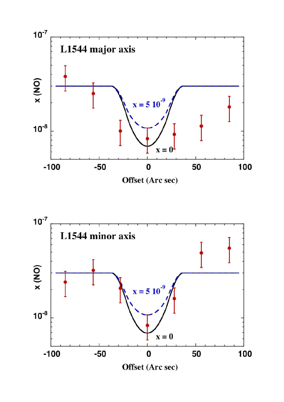
Figure 3: Observed and predicted NO to H₂ column density ratio, $x$(NO) = $N$(NO)/$N$(H₂), for a model of L1544 in which the Tafalla et al. (2002) density distribution (cf. Sect. 4.3) is adopted. Two different assumptions (indicated on the Figure) are made regarding the value of $n$(NO)/$n$(H₂) in the central region, offsets $r\leq 30$${}^{{}^{\prime\prime}}$ (4000 AU): $n({\rm NO})/n({\rm H}_{2})=5\,10^{-9}$ (broken curve); $n({\rm NO})/n({\rm H}_{2})=0$ (full curve). Outside this region, $n$(NO)/$n$(H₂) = $3\,10^{-8}$ is assumed. The filled circles with error bars denote the observed values.

An analogous model for our R.A. cut in L183, in which the Crapsi et al. (2005a) density distribution was adopted (a central density of $10^{6}$ cm^-3 and a power–law decrease in the density beyond a radius of 4200 AU), shows the displacement, to which we alluded above, of the observed minimum of the NO abundance ratio from the dust peak. In this case also, it will be necessary to map fully the NO column density distribution to take the analysis further.

4.2 Chemical considerations

In prestellar cores, the nitrogen chemistry depends on gas–phase conversion of atomic into molecular nitrogen. As was mentioned in the Introduction, the most efficient scheme for this conversion is believed to involve NO as an intermediate, through reactions (1) and (2) above. The ratio of the abundance of NO to that of OH is then given by $k_{1}/k_{2}$, the ratio of the rate coefficients for these reactions.

This relation no longer applies when the atomic nitrogen abundance falls below the value for which the destruction of NO by N, in reaction (2), has the same rate as direct depletion of NO on to the grains, i.e. when

$$n_{\rm H}k_{\rm dep}({\rm NO})=n({\rm N})k_{2},$$

or

$$x({\rm N})\equiv n({\rm N})/n_{\rm H}=k_{\rm dep}({\rm NO})/k_{2}.$$

In these expressions,

$$k_{\rm dep}({\rm NO})=(n_{\rm g}/n_{\rm H})\pi a_{\rm g}^{2}v_{\rm th},$$

where $n_{\rm g}$ is the grain number density, $a_{\rm g}$ is the grain radius, and $v_{\rm th}$ is the thermal speed of the NO molecules. Taking $T=10$ K, we find $k_{\rm dep}({\rm NO})=1.4\times 10^{-18}(0.5/a_{\rm g})$, where $a_{\rm g}$ is in $\mu$m and $k_{\rm dep}$ in cm³ s^-1. With $k_{2}=3.5\times 10^{-11}$ cm³ s^-1 (Baulch et al. 2005), we find that, when the fractional abundance of atomic nitrogen exceeds $x({\rm N})=4\times 10^{-8}$, gas–phase destruction of NO by N dominates, whereas, below this value, NO is removed predominantly by freeze–out on to the grains. A similar argument can be applied to OH, and so the abundances of NO and OH remain related in both regimes.

The rate coefficients for both of the reactions (1) and (2) must be sufficiently large at low temperatures to ensure the conversion of N into N₂, the precursor of N₂H⁺ and NH₃; but the measurement of rate coefficients for neutral–neutral reactions at very low temperatures is demanding (Sims 2005), and so the values of $k_{1}$ and $k_{2}$ remain uncertain. As will be seen in Sect. 4.3, our observations of NO and N₂H⁺ support the existence of a small barrier to reaction (2), which inhibits the destruction of NO by N at temperatures as low as $T=10$ K.

We recall that our observations indicate that, unlike NH₃ and N₂H⁺, NO does not show a constant or even an increasing abundance, relative to H₂, for densities $n_{\rm H}\mathrel{\hbox{\hbox to0.0pt{\hbox{\lower 4.0pt\hbox{$\sim$}}\hss}\hbox{$>$}}}3\times 10^{5}$ cm^-3. Instead, NO appears to decrease in relative abundance approaching the dust emission peak. Here we review some possible chemical explanations of this discrepancy.

• OH may be under–abundant in the high density regions of at least some prestellar cores. This situation could arise for the same reasons that O₂ and water are much less abundant than expected in prestellar cores (see, for example, Pagani et al. (2003), Snell et al. (2000)). Surplus oxygen – that is, oxygen which is not bound in CO – may have frozen out prior to the start of the collapse, giving rise to a situation whereby, once CO has also frozen out, there is more N than O in the gas phase; this assumes that N does not freeze out simultaneously with CO. In the lower density regions, in which CO is still present in the gas phase, the C/O elemental abundance ratio would be close to unity, and the chemistry would have “carbon–rich” characteristics, with, for example, large abundances of cyanopolyynes and similar species. In this case, the main source of atomic oxygen is the reaction of CO with He⁺, which is produced by cosmic ray ionization of He, and hence the fractional abundances of both OH and NO are dependent on the cosmic ray flux. Also, their abundances are determined to some extent by how rapidly atomic oxygen sticks to the grains, an issue which will be discussed in Sect. 4.3 below.

• There may be chemical pathways from N to N₂ which we (and others) have overlooked. Any conversion of N into N⁺, through charge exchange with He⁺, for example, would lead to the production of NH and other hydrides and the subsequent formation of N₂ in neutral–neutral reactions. However, trial calculations which we have carried out suggest that this particular route is not likely to be significant. More promising is the possibility that, under conditions in which the gas–phase abundance of elemental carbon approaches that of elemental oxygen, the reactions

  $${\rm N}+{\rm CH}\rightarrow{\rm H}+{\rm CN}$$ (3)

  and

  $${\rm N}+{\rm CN}\rightarrow{\rm C}+{\rm N}_{2}$$ (4)

  assume importance relative to reactions (1) and (2). We consider this possibility further in Sect. 4.3.

We conclude that the main forms of oxygen (like the main forms of carbon) appear to have frozen on to dust–grain surfaces at densities approaching $10^{6}$ cm^-3 and, moreover, that some form of nitrogen is more volatile and hence more abundant in the gas phase than any form of oxygen. Another conclusion is that, in the densest parts of prestellar cores, oxygen exists mainly as solid H₂O, CO, and perhaps CO₂, with a fractional abundance in the solid state which is larger than the values derived for lower density ($\mathrel{\hbox{\hbox to0.0pt{\hbox{\lower 4.0pt\hbox{$\sim$}}\hss}\hbox{$<$}}}3\times 10^{4}$ cm^-3) material. Having eliminated other possibilities, we arrive at the proposal that atomic nitrogen does not stick effectively to icy dust grains, even at kinetic temperatures close to 10 K (although we note that a small abundance of OH or CH is also necessary to the formation of N₂). This proposal is not in conflict with the recent laboratory studies of Bisschop et al. (2006) and Öberg et al. (2005), which suggest that N₂ freezes out similarly to CO. Then, atomic N is likely to be the main repository of nitrogen in the gas phase.

4.3 Free–fall collapse model

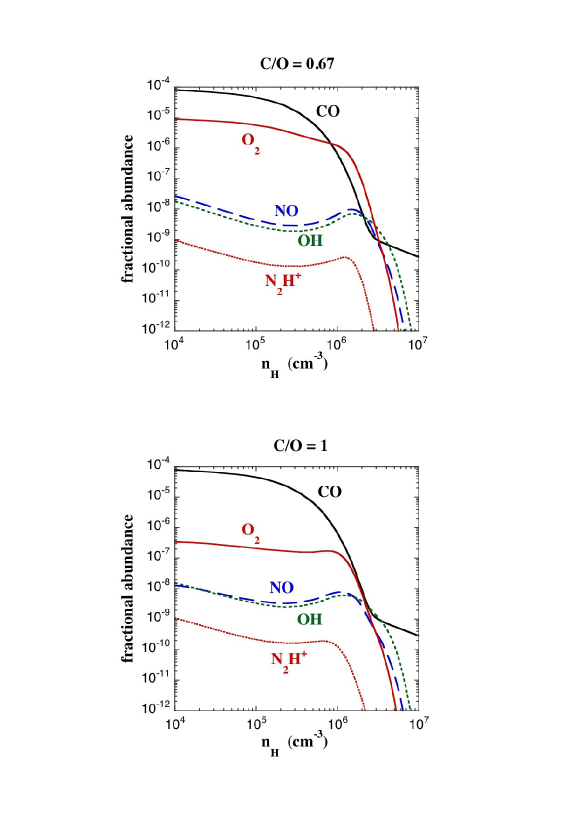
Figure 4: Results of models of the chemistry in a core collapsing on the free–fall timescale. Results are shown for models in which (a) $n_{\rm C}/n_{\rm O}=0.67$ and (b) $n_{\rm C}/n_{\rm O}=0.97\approx 1$ initially. In both cases, the sticking probabilities $S({\rm N})=S({\rm O})=0.1$ and $S=1.0$ for all other neutral species.

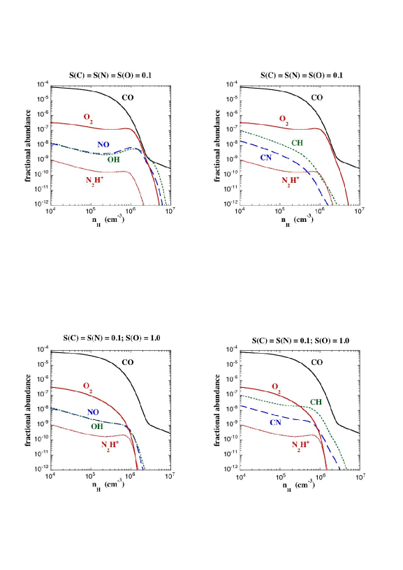
Figure 5: Results of models of the chemistry in a core collapsing on the free–fall timescale. Results are shown for models in which the grain sticking coefficient of atomic oxygen is set equal to $S({\rm O})=0.1$ (upper panels) and $S({\rm O})=1.0$ (lower panels). In both cases, $S({\rm C})=S({\rm N})=0.1$ and $S=1.0$ for all other neutral species; $n_{\rm C}/n_{\rm O}=0.97\approx 1$ initially in the gas phase.

To test some of the above ideas, we have carried out calculations of the variation of NO, N₂H⁺, and NH₃ with density in the framework of the free–fall collapse model presented by Flower et al. (2006). In this study, it was found that a good fit to the observations of L1544 in NH₃, N₂H⁺, and their deuterated isotopes required a grain surface area per H–atom roughly an order of magnitude less than in the diffuse interstellar medium. These simulations assumed a single grain size (radius) of typically 0.5 $\mu$m. It was assumed also that the sticking coefficients for both atomic nitrogen and oxygen are significantly less than unity. Then, NH₃ and N₂H⁺ remain in the gas phase at densities for which CO and other C–containing molecules are already depleted. In the present Section, we use the model developed by Flower et al. (2006) and examine its predictions for the NO abundance. When so doing, we take account of the fact that our observations indicate that NO is intermediate between the C–containing species and molecules like NH₃. The complete chemistry file and list of chemical species are available from http://massey.dur.ac.uk/drf/protostellar/species_chemistry_08_06.

One possibility which has been investigated is that our assumed initial abundances (calculated in steady state for a density $n_{\rm H}=10^{4}$ cm^-3) influence the results significantly. In particular, we have compared our ‘standard model’, in which the ratio of elemental carbon to oxygen in the gas–phase is initially 0.67, to a model in which this ratio approaches 1. In this latter case, the underlying assumption is that oxygen which is not initially in the form of gas–phase CO is in water ice. The results of these calculations are shown in Fig. 4. We see from this Figure that the variation of the fractional abundance of NO, $n({\rm NO})/n_{\rm H}$, with $n_{\rm H}$ is very similar in the two cases; this is because NO forms in the reaction (1) of N with OH. The OH radical is formed and destroyed in binary reactions involving atomic O, and so its fractional abundance is insensitive to the total amount of oxygen in the gas phase. On the other hand, there is a large decrease in the fractional abundance of O₂ when the ratio $n_{\rm C}/n_{\rm O}$ is increased. The computed fractional abundance of O₂ becomes just about compatible with the upper limit of $n({\rm O}_{2})/n({\rm H}_{2})\mathrel{\hbox{\hbox to0.0pt{\hbox{\lower 4.0pt\hbox{$\sim$}}\hss}\hbox{$<$}}}10^{-7}$ derived by Pagani et al. (2003), from observations of a number of prestellar cores, in the ‘carbon–rich’ case. For this reason, we adopted $n_{\rm C}/n_{\rm O}=0.97\approx 1$ initially, in the gas phase, in subsequent models.

We have already mentioned in Sect. 4.2 that N₂ is the precursor of N₂H⁺. Therefore, the initial value of the fractional abundance of N₂H⁺ depends on the initial fractional abundance of N₂. Because reactions (1)–(4), which transform N into N₂, involve minor species, OH and CH, this transformation process is slow, requiring approximately $5\times 10^{6}$ yr to attain equilibrium at a gas density $n_{\rm H}=10^{4}$ cm^-3. Thus, it is far from clear that the ratio $n({\rm N})/n({\rm N}_{2})$ can be assumed to be initially in equilibrium (cf. Flower et al. 2006). Accordingly, we have varied the initial value of this ratio from $n({\rm N})/n({\rm N}_{2})<<1$, obtained assuming that the chemistry has reached equilibrium, to $n({\rm N})/n({\rm N}_{2})>>1$, with a view to improving the agreement with the fractional abundance of N₂H⁺ deduced from our observations.

The observed quantities are the column densities of NO, N₂H⁺ and H₂, as functions of position. In order to compare the free–fall model with the observations, we relate the offset position to the gas density by means of the relation

$$n(r)=\frac{n(0)}{1+(\frac{r}{r_{2}})^{\alpha}}$$

(Tafalla et al. 2002), where $n$ is the gas density, $r$ is the offset from centre, $r=0$, $n(0)$ is the central density of molecular hydrogen, and $r_{2}$ is the radial distance over which the density decreases by a factor of 2, relative to the central density. From the 1.2 mm dust continuum emission map of L1544, Tafalla et al. derived $r_{2}=20$${}^{{}^{\prime\prime}}$(equivalent to 0.014 pc at the distance of L1544), $\alpha=2.5$, and $n(0)=1.4\times 10^{6}$ cm^-3. In view of the freeze–out density indicated by the free-fall model (Fig. 5), we have adopted a central density $n(0)=0.5\times 10^{6}$ cm^-3 of molecular hydrogen, equivalent to $n_{\rm H}(0)=1.0\times 10^{6}$ cm^-3. We consider that the central density is uncertain to at least this factor of 2.8 (cf. Bacmann et al. 2000, Crapsi et al. 2005a, Doty et al. 2005). We note also that the density $n(r)$ which derives from the above expression is the maximum value along the line of sight at a given offset, $r$, from centre.

From our earlier discussion (Sect. 4.2), we see that NO might be sensitive also to the sticking coefficient of atomic oxygen, $S$(O), and so we compare results for $S({\rm O})=0.1$ and $S({\rm O})=1.0$ in Fig. 5. The results of the calculations are, indeed, sensitive to $S$(O): NO vanishes from the gas phase at a density of roughly $10^{6}$ cm^-3 when $S({\rm O})=1.0$ but survives to at least 3 times that density when $S({\rm O})=0.1$. Of course, CO is unaffected by the oxygen sticking probability. In these calculations, $S({\rm C})=S({\rm N})=0.1$ and $S=1.0$ for all other neutral species. The model is ‘carbon–rich’ ($n_{\rm C}/n_{\rm O}=0.97$ initially in the gas phase), and hence the route to N₂, through the reactions of CH and CN with N (reactions (3) and (4)), assumes importance, relative to the reactions of OH and NO with N (reactions (1) and (2)). The initial abundance of CH exceeds that of OH by an order of magnitude. It is noticeable that CH and CN are considerably more abundant at densities of the order of 10⁶ cm^-3 in the models in which $S({\rm O})=1.0$; atomic oxygen destroys these species, forming CO. A consequence is that, if $S({\rm O})$ is large, CN may be expected to be depleted less than other C–containing species towards the density peaks of prestellar cores. Finally, we see that the close link between the fractional abundances of NO and OH, mentioned in the Introduction and discussed in Sect. 4.2, is apparent in Fig. 5.

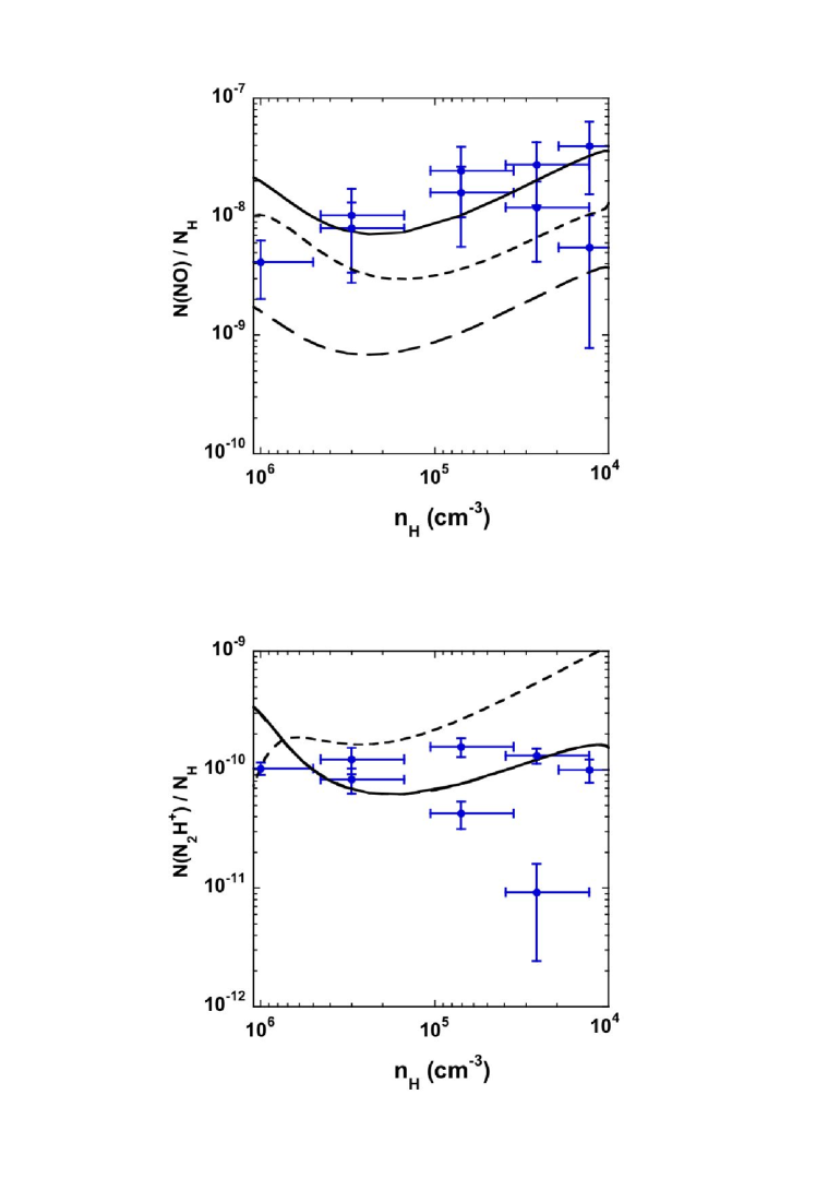
Figure 6: A comparison of the column densities of NO and N₂H⁺, relative to N${}_{\rm H}\approx 2N({\rm H}_{2})$, derived from observations along the minor axis of L1544 (points with error bars), with the fractional abundance of NO, $n({\rm NO})/n_{\rm H}$, and of N₂H⁺, $n({\rm N}_{2}{\rm H}^{+})/n_{\rm H}$, predicted by free–fall models in which the initial value of the ratio $n({\rm N})/n({\rm N}_{2})$ is varied from its equilibrium value, $n({\rm N})/n({\rm N}_{2})=1/60$ (dashed curve) to $n({\rm N})/n({\rm N}_{2})=18$ (long–dashed curve). The effect of introducing a small (26 K) barrier in the rate coefficient of the reaction of NO with N (reaction (2)) is also illustrated (full curve); the introduction of the barrier has no perceptible effect on N₂H⁺, where the long–dashed and full curves overlap. In these calculations, $S({\rm C})=S({\rm N})=S({\rm O})=0.1$ and $S=1.0$ for all other neutral species; initially, $n_{\rm C}/n_{\rm O}=0.97\approx 1$ in the gas phase. Note that the abscissa has been reversed to reflect the decrease of the density with increasing distance from the centre.

In Fig. 6 are compared the observed values of the column density ratios $N({\rm NO})/N_{\rm H}$ and $N({\rm N}_{2}{\rm H}^{+})/N_{\rm H}$, where $N_{\rm H}=2N({\rm H}_{2})$, with the computed values of the fractional abundances $n({\rm NO})/n_{\rm H}$ and $n({\rm N}_{2}{\rm H}^{+})/n_{\rm H}$. In this Figure, $S({\rm C})=S({\rm N})=S({\rm O})=0.1$. The horizontal error bars represent a factor of 3 uncertainty in $n_{\rm H}$, whilst the vertical error bars incorporate the observational uncertainties in the line intensity or flux measurements, together with an assumed 15 percent calibration error. The observed points fall on two branches, corresponding to opposite sides of the central position. The emission from L1544 is observed to be asymmetric about the centre, whereas the empirical model of the density distribution, given above, assumes radial symmetry. (The lower branch corresponds to negative offsets (in R.A.) for both NO and N₂H⁺.) It may be seen that increasing the initial value of the atomic to molecular nitrogen ratio has the effect of yielding much improved agreement between the observed and computed profiles of N₂H⁺. On the other hand, the profile of NO is displaced downwards, owing to the enhanced rate of its destruction by N, and the computed profile now falls well below the observations. However, if a small barrier introduced into the rate coefficient for the reaction of NO with N, the computed NO profile becomes once again compatible with the observations, as may be seen in Fig. 6. In the calculations presented in this and the following Figures, we have adopted the rate coefficient for the reaction of NO with N which is given in the current version of the UMIST chemical reaction database (LeTeuff et al. 2000), rate05, namely $k_{2}=3.75\times 10^{-11}{\rm exp}(-26/T)$ cm³ s^-1, which derives from the study of Duff & Sharma (1996). This small reaction barrier is sufficient to inhibit the destruction of NO by N significantly at $T=10$ K. We note that it is presently very difficult to confirm or exclude the existence of such a small barrier by either laboratory measurements, which extend to insufficiently low temperatures, or theoretical calculations, which would need to determine the transition state energy to an accuracy of 100 $\mu$h.

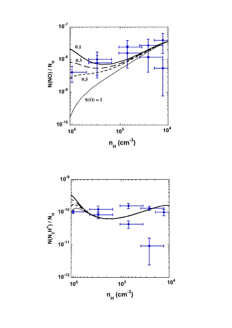
Figure 7: A comparison of the column densities of NO and N₂H⁺, relative to N${}_{\rm H}\approx 2N({\rm H}_{2})$, derived from observations along the minor axis of L1544 (points with error bars), with the fractional abundance of NO, $n({\rm NO})/n_{\rm H}$, and of N₂H⁺, $n({\rm N}_{2}{\rm H}^{+})/n_{\rm H}$, predicted by free–fall models in which the grain sticking coefficient of atomic oxygen is varied: $S({\rm O})=0.1,0.3,0.5,1.0$. In all cases, $S({\rm C})=S({\rm N})=0.1$ and $S=1.0$ for all other neutral species; initially, $n_{\rm C}/n_{\rm O}=0.97\approx 1$ in the gas phase, and $n({\rm N})/n({\rm N}_{2})=18$. Note that the abscissa has been reversed to reflect the decrease of the density with increasing distance from the centre.

In Fig. 7, we investigate the effect of varying the grain sticking coefficient of atomic oxygen, in the range in the range $0.1\leq S({\rm O})\leq 1.0$. Once again, $S({\rm C})=S({\rm N})=0.1$. We see that the general trends of the observations are for $N({\rm NO})/N_{\rm H}$ to increase with decreasing density (increasing distance from the centre), whereas $N({\rm N}_{2}{\rm H}^{+})/N_{\rm H}$ remains approximately constant or, possibly, tends to decrease with decreasing density; this is in accord with the comments made in the previous Section. The models in which $S({\rm O})>0.1$ predict that the fractional abundance of N₂H⁺ is roughly constant, which, given the large error bars, is in reasonable accord with the observations. As $S({\rm O})$ increases towards unity, the amount of oxygen remaining in the gas phase at high densities decreases and the rate of formation of NO, in reactions (1) and (2), decreases also. When $S({\rm O})=0.5$, $n({\rm NO})/n_{\rm H}=3.5\times 10^{-8}$ when $n_{\rm H}=10^{4}$ cm^-3, and $n({\rm NO})/n_{\rm H}=2.9\times 10^{-9}$ when $n_{\rm H}=10^{6}$ cm^-3; these values are consistent with those deduced from the empirical model (Sect. 4.1). However, we wish to emphasize that we do not consider ourselves in a position to “determine” the sticking coefficients: this should be done in the laboratory. We have treated the sticking coefficients of C, N, and O simply as parameters of the model, varying their values in an attempt at fitting the available observations.

In our recent study (Flower et al. 2006), we found that satisfactory agreement could be obtained with the observed high levels of deuteration of the nitrogen–containing species NH₃ and N₂H⁺, providing that the grains were sufficiently large ($a_{\rm g}\approx 0.50$ $\mu$m, as in the present calculations) and that the sticking probabilities of atomic nitrogen and atomic oxygen were both less than unity ($S\mathrel{\hbox{\hbox to0.0pt{\hbox{\lower 4.0pt\hbox{$\sim$}}\hss}\hbox{$<$}}}0.3$). For the reasons given above, we have since modified the initial values of the C/O and N/N₂ ratios, as well as reducing the sticking probability of atomic carbon to $S({\rm C})=0.1$. We have seen (Fig. 7) that the observed variations of the column densities of NO and N₂H⁺ can then be reproduced, but it is necessary to establish that this success is not at the expense of the earlier agreement with the degrees of deuteration of NH₃ and N₂H⁺.

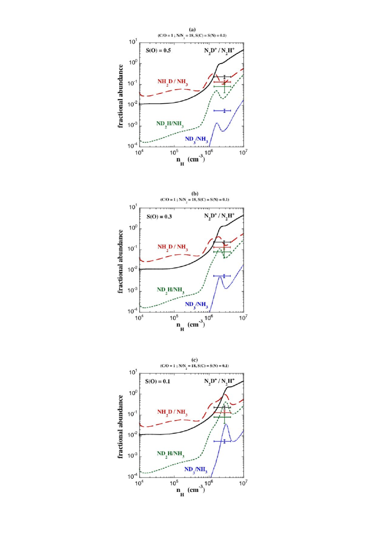
Figure 8: The abundance ratios of the deuterated forms of N₂H⁺ and NH₃, as functions of $n_{\rm H}$, together with the values observed in the prestellar core L1544 (cf. Flower et al. 2006, figure 5c). The grain sticking probability of atomic oxygen, $S({\rm O})=0.5,0.3,0.1$ in panels (a), (b), (c), respectively. In all cases, $S({\rm C})=S({\rm N})=0.1$ and $S=1.0$ for all other neutral species; initially, $n_{\rm C}/n_{\rm O}=0.97\approx 1$ in the gas phase, and $n({\rm N})/n({\rm N}_{2})=18$.

In Fig. 8 are plotted the relative abundances of the deuterated and non-deuterated forms of NH₃ and N₂H⁺ which derive from the present calculations, adopting $n_{\rm C}/n_{\rm O}=0.97$ and $n({\rm N})/n({\rm N}_{2})=18$ initially, together with $S({\rm C})=S({\rm N})=0.1$; the sticking probability of atomic oxygen is varied in the range $0.1\leq S({\rm O})\leq 0.5$. The observational points and their error bars are identical to those adopted in our earlier paper (Flower et a. 2006, figure 5c). It may be seen from Fig. 8 that satisfactory agreement with the observed levels of deuteration is still obtained when $S({\rm O})\approx 0.3$. This Figure emphasizes the fact that the degree of deuteration of NH₃ increases with increasing gas density. The fractional abundance of ND₃, for example, has a distinct maximum at densities of order $10^{6}$ cm^-3. As kinematical parameters, such as the collapse speed, might be expected to vary with radial distance (and hence density) in the core, the widths of emission lines from successive stages of deuteration of NH₃ could provide information on the variation of the infall speed with the gas density.

We note that the effect of subsequent coagulation on the size of initially large grains – specifically, $a_{\rm g}=0.50$ $\mu$m in the present models – is small, over the range of compression considered ($10^{4}\leq n_{\rm H}\leq 10^{7}$ cm^-3), and has little consequence for the freeze–out timescale.

5 Concluding remarks

Our principal observational conclusion is that NO, unlike NH₃ and N₂H⁺, is depleted towards the density peaks of the prestellar cores L1544 and L183. This result was surprising, in that NO was believed to be an important intermediate of the nitrogen chemistry. In particular, the path from atomic to molecular nitrogen was believed to involve both OH and NO. Our results cast some doubt on this assumption, suggesting that molecular nitrogen may form from CH and CN at high densities. If so, CN is an important intermediate in the nitrogen chemistry. Further mapping of CN in prestellar cores, extending the observations of L183 by Dickens et al. (2000), would be extremely useful. Our models suggest a fractional abundance $n({\rm CN})/n_{\rm H}\approx 10^{-10}$ towards the peak of L1544, corresponding to a column density of the order of $10^{13}$ cm^-2. In the case of L183, the central depression in the fractional abundance of NO is offset from the dust peak. This object needs further study: complete maps of the NO distribution are required.

In an attempt to explain our observations within the framework of a free–fall collapse model, we have varied the values of the sticking probabilities of atomic C, N and O, and also the initial values of the elemental C/O and the atomic to molecular nitrogen abundance ratios in the gas phase. We find that

• the prestellar core L1544 is likely to be ‘carbon–rich’, in the sense that $n_{\rm C}/n_{\rm O}\approx 1$ in the gas phase. An initial $n_{\rm C}/n_{\rm O}=0.97$ leads to values of $n({\rm O}_{2})/n({\rm H}_{2})$ which are in much better agreement with the observed upper limits than when the gas is oxygen–rich ($n_{\rm C}/n_{\rm O}=0.67$).

  In objects in which the gas–phase C/O abundance ratio is close to unity, the fractional abundances of C–rich species, such as the cyanopolynes, are expected to be enhanced relative to oxygen–containing species, such as O₂ and H₂O. Of the two cores which we have studied, this is true of L1544 (cf. Walmsley et al. 1980), whereas L183 is relatively carbon–poor (cf. Swade 1989).

• The ratio $n({\rm N})/n({\rm N}_{2})$ at the start of collapse is much more than its value in equilibrium. This result is perhaps not surprising, given the long timescale ($\approx 5\times 10^{6}$ yr) required for the nitrogen chemistry to reach equilibrium at densities $n_{\rm H}\approx 10^{4}$ cm^-3. We note that Maret et al. (2006) have recently and independently arrived at essentially the same conclusion, viz. that most of the nitrogen in the gas phase is atomic, also from an analysis of observations of N₂H⁺, in their case in the prestellar core B68 (but with implications for the deficiency of molecular nitrogen in cometary ices). If $n({\rm N})/n({\rm N}_{2})>>1$ in the gas phase, then our observations of NO imply the existence of a small barrier ($\approx 25$ K) to the reaction of NO with N (equation (2)). Experimental demonstration of the existence of such a small barrier to this and, possibly, the other key neutral–neutral reactions (1), (3) and (4), whilst difficult to achieve, is highly desirable.

• The grain sticking probabilities of atomic C, N and, probably, O are significantly smaller than unity; values of $S({\rm C})=S({\rm N})=0.1$ and $0.1\leq S({\rm O})\leq 1.0$ were adopted in the calculations reported above. However, the assumed values of the sticking probabilities for the atomic species are ad hoc and require confirmation by means of experimental measurements. Such measurements should presumably be made on CO ice, as in the experiments of Bisschop et al. (2006).

Appendix A Determination of the column densities

The method for deriving the column density of NO, from observations of the hyperfine components of rotational transitions, assumed optically thin, has been presented by Gerin et al. (1992); we followed their method in the present paper. The case of N₂H⁺ was considered by Caselli et al. (2002), who gave expressions for the total column density of N₂H⁺, for the case of a finite optical depth in the line and also in the optically thin limit, in their Appendix A. If the optical depth in a line of central frequency $\nu$ and wavelength $\lambda$ is finite, then the total column density of the molecular ion is related to to the optical depth $\tau$ at the line centre by

$$N=\frac{4\pi\Delta v}{\lambda^{3}}\left(\frac{\pi}{{\rm ln}\,2}\right)^{\frac{1}{2}}\frac{Q}{g_{\rm u}A({\rm u}\rightarrow{\rm l})}\frac{\tau}{1-\exp(-h\nu/k_{\rm B}T_{\rm ex})}\frac{1}{\exp(-E_{\rm l}/k_{\rm B}T_{\rm ex})}$$ (5)

where $\Delta v$ is the full width of the line at half-maximum intensity (the line profile is assumed to be gaussian), $g_{\rm u}$ is the degeneracy (statistical weight) of the upper level of the observed transition, $A({\rm u}\rightarrow{\rm l})$ is the spontaneous radiative transition probability to the lower level, whose excitation energy is $E_{\rm l}$; $Q$ is the partition function, considered below. We have assumed implicitly a Boltzmann distribution of population at an excitation temperature (to be determined) $T_{\rm ex}$. In the limit of low optical depth at the line centre, the expression for the total column density is

$$N=\frac{4\pi\Delta v}{\lambda^{3}}\left(\frac{\pi}{{\rm ln}\,2}\right)^{\frac{1}{2}}\frac{Q}{g_{\rm u}A({\rm u}\rightarrow{\rm l})}\frac{(k_{\rm B}T_{\rm mb}/h\nu)}{[\exp(h\nu/k_{\rm B}T_{\rm ex})-1]^{-1}-[\exp(h\nu/k_{\rm B}T_{\rm bg})-1]^{-1}}$$

$$\times\frac{1}{1-\exp(-h\nu/k_{\rm B}T_{\rm ex})}\frac{1}{\exp(-E_{\rm l}/k_{\rm B}T_{\rm ex})}$$ (6)

where $T_{\rm mb}$ is the main beam brightness temperature and $T_{\rm bg}$ is the temperature of the background radiation field, usually taken to be a black–body at $T_{\rm bg}=2.73$ K.

The line width, $\Delta v$, and the brightness temperature, $T_{\rm mb}$, refer to a given component of the $J=1\rightarrow 0$ multiplet, which is observed towards L1544 and L183 to comprise seven resolved components. The full set of transitions is listed in Table 4, along with the corresponding line strengths. A comparison of the relative intensities of the components with the values expected in the optically thin limit (when they are given by the line strengths) shows that some of the lines are optically thick towards the dust emission peaks of these two sources. Accordingly, we have used the weakest transition, $J,F_{1},F=1,1,0\rightarrow 0,1,1$ of the multiplet, which should also be the most optically thin, to determine the column density of N₂H⁺. Previous work has shown that N₂H⁺ column densities derived in this way agree to within about 30 percent with the results of more sophisticated analyses of the emission in the rotational multiplet, which allow for optical depth effects; this is the case even at the peak of the emission, where the assumption that the $1,1,0\rightarrow 0,1,1$ transition is optically thin is least valid. Crapsi et al. (2005a) estimated the“total” optical depth (i.e. summed over all seven components) of the N₂H⁺ $J=1\rightarrow 0$ multiplet to be $\tau=12.6\pm 0.7$ towards the peak of L1544, which corresponds to an optical depth in the $1,1,0\rightarrow 0,1,1$ transition of $12.6/27=0.47$ and an escape probability of 0.80 (and hence a 25 percent underestimation of the column density owing to the “optically thin” assumption). They estimated, also from their fit, an excitation temperature $T_{\rm ex}=5$ K for the $J=1\rightarrow 0$ multiplet in N₂H⁺.

The hyperfine splitting of the rotational energy levels of ¹⁴N₂H⁺ arises from the interaction of the spin angular momentum, ${\bf I}$, of the nitrogen nuclei and the rotational angular momentum, ${\bf J}$, of the molecule. The angular momentum coupling scheme is

$${\bf F_{1}}={\bf J}+{\bf I_{1}}$$

and

$${\bf F}={\bf F_{1}}+{\bf I_{2}}$$

The nuclear spin angular momentum quantum number is $I_{1}=I_{2}=1$. When $J\geq 1$, there are three possible values of $F_{1}$, namely $F_{1}=J-1,J,J+1$. On the other hand, when $J=0$, $F_{1}=I_{1}=1$. The possible values of $F$, the total angular momentum, are determined by the (weaker) coupling to the spin of the second (inner) nitrogen nucleus. The quantum numbers $J,F_{1},F$ which identify the hyperfine levels of the $J=1$ and $J=0$ rotational states are listed in Table 4. The optically allowed transitions are determined by the electric dipole selection rules $\Delta F=0,\pm 1$ (but $\Delta F=0$, when $F=0$, is not allowed) governing the change in $F$ in the transition. The hyperfine splitting of $J=0$, which arises from the nuclear spin–spin interaction, is very small: see Green et al. (1974), Caselli et al. (1995). Consequently, allowed transitions from a given upper level, $J=1,F_{1},F$, are unresolved, and there remain seven resolved hyperfine transitions between $J=1$ and $J=0$, one from each of the hyperfine levels of $J=1$.

The partition function, $Q$, which appears in equation (6), is defined by

$$Q=\sum_{i}g_{i}\exp\left(-\frac{E_{i}}{k_{\rm B}T_{\rm ex}}\right)$$ (7)

where the summation extends over all energy levels, and $g_{i}=2F_{i}+1$. As $E_{i}$ is approximately the same for all hyperfine levels belonging to the same $J$, the summation over $g_{i}$ for each value of $J$ may be carried out, yielding

$$Q=9\sum_{i}g_{J}\exp\left(-\frac{E_{J}}{k_{\rm B}T_{\rm ex}}\right)$$ (8)

where $g_{J}=2J+1$. The factor of 9 appearing in (8) is the product of the degeneracies, $2I+1=3$, arising from the spin of the nitrogen nuclei. It may be verified that, for a given value of $J$,

$$\sum_{i}(2F_{i}+1)=9\,(2J+1)$$ (9)

Assuming that the hyperfine splitting is small compared with the rotational splitting of the energy levels (which is verified, in practice), the relationship between the probability of a given hyperfine transition within a rotational multiplet and the total probability of a transition between the rotational levels $J^{\prime}$, $J$ is

$$g_{F^{\prime}}A(J^{\prime}F_{1}^{\prime}F^{\prime}\rightarrow JF_{1}F)=9\,g_{J^{\prime}}A(J^{\prime}\rightarrow J)S(F_{1}^{\prime}F^{\prime},F_{1}F)$$ (10)

where $g_{F^{\prime}}=2F^{\prime}+1$ and $g_{J^{\prime}}=2J^{\prime}+1$; $9\,g_{J^{\prime}}$ is the total degeneracy of rotational state $J^{\prime}$ (cf. equation (9)). $S(F_{1}^{\prime}F^{\prime},F_{1}F)$ is the line strength, which determines the relative intensities of the hyperfine components of the rotational multiplet. The sum of the line strengths, over all components of the multiplet, is equal to unity. Because the hyperfine levels of $J=0$ are almost degenerate, the line strengths may be summed over over all allowed transitions from a given hyperfine level of $J=1$. In Table 4, the resulting line strengths are listed for the seven resolved transitions from $J^{\prime}=1$ to $J=0$ in N₂H⁺; they may be seen to be given by the ratio $(2F^{\prime}+1)/\sum(2F^{\prime}+1)$, where the summation extends over the hyperfine levels of the upper rotational state, $J^{\prime}$. When $J^{\prime}=1$, $\sum(2F^{\prime}+1)=27$, as may be seen from equation (9); see Townes & Shawlow (1955) and Tatum (1986) for more detailed discussions of coupling schemes and line strengths. The specific case of N₂H⁺ is considered in a recent publication of Daniel et al. (2006) (but note that $J^{\prime}$ in their equation (1) for the transition probability should read $J$).

Table 4: The $J^{\prime}=1\rightarrow J=0$ hyperfine transitions at 93.2 GHz. The seven resolved lines are ordered in increasing frequency, from bottom to top. For each transition, the quantum numbers identifying the upper level (with primes) and lower level are given, along with the corresponding line strength. The line strengths have been summed over the allowed transitions from a given hyperfine level of $J=1$, given that the hyperfine levels of $J=0$ are almost degenerate.

Transition	Line strength
$J^{\prime}F_{1}^{\prime}F^{\prime}\rightarrow JF_{1}F$	$S(F_{1}^{\prime}F^{\prime},F_{1}F)$
$101\rightarrow 012$	$1/9$
$121\rightarrow 011$	$1/9$
$123\rightarrow 012$	$7/27$
$122\rightarrow 011$	$5/27$
$111\rightarrow 010$	$1/9$
$112\rightarrow 012$	$5/27$
$110\rightarrow 011$	$1/27$

The derivation of the total column density of a molecule from observations of individual transitions – hyperfine transitions between rotational states in the cases of NO and N₂H⁺ – relies on correcting for the populations of unobserved levels. When this is done via equation (7) for the partition function, $Q$, it is assumed that the relative level populations may be characterized by a Boltzmann distribution at the excitation temperature, $T_{\rm ex}$; this is the case when collisional de-excitation of the upper to the lower rotational state dominates spontaneous radiative decay. The ‘critical density’ is defined as the density of the collisional perturber (predominantly H₂ in the case of rotational transitions) for which the radiative and collisional decay rates become equal (once a correction has been made for the photon escape probability). For perturber densities higher than the critical density, a Boltzmann distribution of the relative level populations is approached, at the kinetic temperature of the gas. Corrections can be made for optical depth effects by means of either “large velocity gradient” programs (e.g. Crapsi et al. 2004) or more sophisticated (Monte–Carlo) radiative transport models (e.g. Tafalla et al. 2002).

The peak column density of N₂H⁺ in L1544 derived by Crapsi et al. (2005a), $N$(N₂H⁺) $=(1.83\pm 0.19)\times 10^{13}$ cm^-2, who used the weakest component and the optically thin approximation, agrees to within the error bar with the determination of Caselli et al. (2002), $N$(N₂H⁺) $=2.0\times 10^{13}$ cm^-2, who used all seven hyperfine components and corrected for the finite optical depths. Thus, a simple approach to the determination of the column density of N₂H⁺ can yield satisfactory results. To our knowledge, all line transfer models to date have assumed that the density structure of L1544 can be represented by a one–dimensional, spherically symmetric distribution. It would be interesting to compare with the predictions of radiative line transfer models which go beyond the approximation of a single dimension, even though the angular resolution and completeness of the currently available maps of the molecular emission would constrain the comparison of such models with the observations.

We are not aware of calculations of rate coefficients for rotational transitions in NO, induced by H₂. However, calculations have been performed for OH – H₂ (Offer & van Dishoeck 1992), which shares many physical characteristics with NO – H₂, not least in the rotational structure of the target molecule. In the case of collisions with para–H₂, which is the main form of H₂ at low temperatures, the calculations of Offer & van Dishoeck (1992) indicate that the rate coefficient for rotational de-excitation at $T=50$ K is of the order of $10^{-11}$ cm³ s^-1 and not strongly dependent on the kinetic temperature, $T$. The rate of spontaneous radiative decay in the transitions of NO which we observed (cf. Table 1) is of the order of $10^{-7}$ s^-1 (Gerin et al. 1992), which implies a critical density of H₂ of the order of $10^{4}$ cm^-3. In the regions of the protostellar cores considered above, $n({\rm H}_{2})\mathrel{\hbox{\hbox to0.0pt{\hbox{\lower 4.0pt\hbox{$\sim$}}\hss}\hbox{$>$}}}10^{4}$ cm^-3, extending up to values in excess of $10^{6}$ cm^-3. We conclude that the assumption of Boltzmann equilibrium at the local kinetic temperature is justified in the case of NO.

Consider now N₂H⁺. Daniel et al. (2005) have recently computed rate coefficients for the rotational de-excitation of N₂H⁺ by He; in the absence of data specifically for H₂, we adopt their results as a guide. Their calculations indicate a value of $10^{-11}$ cm³ s^-1 for rotational transitions in N₂H⁺, induced by He, at low temperatures, similar to the value above for NO – H₂. On the other hand, the rate of spontaneous decay of $J=1$ to $J=0$ is of the order of $10^{-5}$ s^-1 (Dickinson & Flower 1981), 2 orders of magnitude larger than for NO (N₂H⁺ has a much larger dipole moment). Consequently, the critical density for N₂H⁺ is of the order of $10^{6}$ cm^-3, although line trapping will tend to reduce this value towards the peaks of L1544 and L183.