Protoplanet Magnetosphere Interactions

Abstract

Aims. In this paper, we study a simple model of an orbiting protoplanet in a central magnetospheric cavity, the entry into such a cavity having been proposed as a mechanism for halting inward orbital migration.

Methods. We have calculated the gravitational interaction of the protoplanet with the magnetosphere using a local model and determined the rate of evolution of the orbit.

Results. The interaction is found to be determined by the outward flux of MHD waves and thus the possibility of the existence of such waves in the cavity is significant.

Conclusions. The estimated orbital evolution rates due to gravitational and other interactions with the magnetosphere are unlikely to be significant during protoplanetary disk lifetimes.

1 Introduction

The discovery of extrasolar giant planets orbiting close to their host stars ( Mayor & Queloz 1995; Marcy & Butler 1995, 1998) with periods of a few days has led to the proposal that orbital migration during and post formation is responsible for them attaining short period orbits. This is because of the difficulties associated with forming such planets in situ, either in the critical core mass accumulation followed by gas accretion scenario, or the gravitational instability scenario for giant planet formation (see Papaloizou & Terquem 2006 and references therein for more discussion). However, estimates of disk driven migration time scales have in general found these to be short compared to protostellar disk lifetimes (e.g. Nelson et al. 2000). This in turn suggests the need for a mechanism to halt migration so preventing the protoplanet from falling into the star. Lin Bodenheimer & Richardson (1996) suggested that entry into a stellar magnetosphere close to the star could provide such a mechanism. This is through detachment from the disk. Indeed once the protoplanet is interior to the 2:1 resonance with the inner disk edge, interaction with the disk would be expected to cease through the lack of effective outer Lindlbad resonances (see e.g. Lin & Papaloizou 1993).

However, there has as yet been no detailed analysis of the expected orbital evolution of protoplanets in magnetospheric cavities or demonstration of the effectiveness of this mechanism for halting inward orbital migration. This would require consideration of models for this inner region and a calculation of the interaction with the protoplanet and the effects on the protoplanet orbit. It is the purpose of this paper to make some first steps in this direction.

Accretion on to T Tauri stars is indeed thought to be magnetically dominated close to the central star in some cases (Cameron & Campbell 1993; Menard et al. 2003). Surface field strengths of a few kilogauss (e.g. Safier 1998; Johns-Krull et al. 1999) have been estimated. According to models of accretion flows with their central regions dominated by the magnetic field of the central star ( e.g. Ghosh & Lamb 1978; Cameron & Campbell 1993; Matt & Pudritz 2004) , at large radii the accretion flow is that of a normal viscous accretion disk ( e.g. Pringle 1981). The magnetic field penetrates the disk due to diffusion arising from the growth of various instabilities. At large radii the magnetic field is weak such that viscous stresses are more important than magnetic stresses. Then the effect of the magnetic field on the disk structure can be ignored. However, at smaller radii the dominance of magnetic stresses leads to the truncation of the disk at a radius, $R_{\rm d,}$ and the channeling of the flow to the star along stellar magnetic field lines.

In order for accretion on to the central star to proceed the magnetic field must not disrupt the disk exterior to the corotation radius, where the angular velocity in the disk coincides with that of the star, since the magnetic torque on the disk would impart angular momentum to the disk gas, making it unable to connect to the stellar field. If disk disruption occurs too far inside corotation the radius, there is an accretion torque acting to spin up the star. In general one can expect there to be an equilibrium state where spin up torques due to accretion and spin down torques due to magnetic stresses acting on the disk cancel. Because of the expected rapid increase of the magnetic stresses as the distance to the star decreases, one expects that $R_{\rm d}$ is slightly less than the corotation radius (Ghosh & Lamb 1978) when the system accretes onto the central star and is near equilibrium.

This general picture of magnetic accretion has been found in recent three dimensional numerical simulations (see Romanova et al. 2004; 2006; Bouvier et al. 2006). It has been found that accretion along field lines takes place in funnel stream flows. When the stellar field is a dipole that is either not nearly aligned or strongly misaligned with the angular momentum axis, the magnetospheric density is relatively low in the equatorial plane. For both small and large misalignment angles, relatively high density streams may occur there. The latter situation may be less favourable for stalling migration as interaction with the protoplanet is potentially stronger.

The purpose of this paper is to consider a simple model of the stellar magnetosphere with a steady state accretion flow and to use it to calculate the protoplanet magnetosphere interaction and the consequent protoplanet orbital evolution rate. This is to establish to what extent entry into such a magnetosphere is by itself sufficient to halt migration without the need to postulate additional effects such as residual coorbital torques resulting from the inner disk edge ( e.g. Masset et al. 2006).

The plan of the paper is as follows: In section 2 we give the basic equations of the problem. In section 3 we consider perturbation of a steady state magnetosphere by a protoplanet in circular orbit with the aim of evaluating the exchange of energy with the orbit resulting from the perturbed gravitational forces.

We carry out a purely local calculation of the protoplanet magnetosphere interaction. This confirms the importance of the existence of propagating waves in order to obtain a non zero energy exchange rate. When the flow is highly super sonic and super Alfvénic the interaction can be described using the well known dynamical friction formalism of Chandrasekhar (1943) and Tremaine & Weinberg (1984). However, when the flow speed is below that of the fast magnetosonic speed but significantly exceeds the slow magnetosonic speed, as in our case, the energy exchange rate is found to be reduced. This is particularly the case when the relative velocity between gas and protoplanet is parallel or nearly parallel to the magnetic field. A similar reduction would be expected to apply to the accretion rate by the protoplanet.

Using the conservation of energy applied to the fluid perturbations in a more general context, we find that the energy exchange rate with the orbit is determined by advected and wave energy fluxes at the system boundaries, confirming the importance of the existence of propagating waves and the boundary conditions for the determination of the energy exchange rate with the orbit.

In section 4 we discuss our results, showing that, for parameters expected for protoplanetary disks, these imply negligible orbital evolution for protoplanets interior to magnetospheric cavities. This in turn implies that if entry into a magnetospheric cavity is responsible for a lack of further migration of a single protoplanet, the orbital elements could subsequently only be affected by stellar tides. Finally we summarise our conclusions.

2 Basic Equations

The basic equations are the equations of ideal MHD in a frame rotating with uniform angular velocity ${{\bf e_{3}}}\Omega_{*},$ where, adopting cylindrical polar coordinates $(r,\varphi,z)$ with origin at the central star, ${{\bf e_{3}}}$ denotes the unit vector in the $z$ direction and $\Omega_{*}$ is the angular velocity of the central magnetospheric region, taken to coincide with that of the central star.

The equation of motion can be written in the form

$${\partial{\bf v}\over\partial t}+{\bf v}\cdot\nabla{\bf v}+2\Omega_{*}{{\bf e_{3}}}\times{\bf v}={\bf f},$$ (1)

where the force per unit mass is given by

$${\bf f}=-{{\nabla P}\over\rho}-\nabla\Phi+{(\nabla\times{\bf B})\times{\bf B}\over 4\pi\rho},$$ (2)

the induction equation in the form

$${\partial{\bf B}\over\partial t}=\nabla\times({\bf v}\times{\bf B})$$ (3)

and the continuity equation in the form

$${\partial\rho\over\partial t}+\nabla\cdot(\rho{\bf v})=0.$$ (4)

Here $\rho$ is the density, $P$ is the pressure, ${\bf v}$ is the velocity and the magnetic field is ${\bf B}.$

When the only source of gravity is the central star treated as a point mass, the combined gravitational and centrifugal potential is

$$\Phi=-{GM_{*}\over\sqrt{r^{2}+z^{2}}}-{1\over 2}\Omega_{*}^{2}r^{2},$$ (5)

with the central stellar mass being $M_{*}$ and $G$ the gravitational constant. For the model considered here we adopt an isothermal equation of state so that $P=\rho c^{2}$ with $c$ being the constant sound speed. We take this to be characteristic of the outer disk so that it will be much less than the orbital speed or a characteristic Alfvén speed.

3 Perturbation Due to an Orbiting Protoplanet

3.1 Angular Momentum Transport and Equilibrium Stellar Spin

We consider the perturbation of a magnetosphere interior to an accretion disk through which matter accretes at a constant or slowly varying rate by an orbiting protoplanet. When a quasi-steady state has been reached, the disk is expected to be disrupted at a radius, $R_{d}$ slightly interior to the corotation radius, $r_{0}$ where the stellar angular velocity coincides with the Keplerian angular velocity expected in the disk. This is given by

$$r_{0}=(GM_{*}/\Omega_{*}^{2})^{1/3}.$$ (6)

In the inner region the flow is expected to become magnetically dominated and sub Alfv’enic (Ghosh & Lamb 1978). This general behaviour with the magnetospheric radius being $\sim 0.85r_{0}$ has been found in recent simulations (see Bouvier et al. 2006). It has also been estimated that the time required to attain such a quasi steady state is short compared to the lifetime of the disk (e.g. Cameron & Campbell 1993; Armitage & Clarke 1996). For a steady state flow (3) and (4) imply that ${\bf v}$ and ${\bf B}$ are parallel.

3.2 Local Analysis

Finding the response of a general steady state magnetospheric accretion flow to an orbiting protoplanet is a very difficult problem. Accordingly we consider possible simplifications. In this section we consider the calculation of the response using a local approximation. The idea behind this is that at any stage, the protoplanet moves relative to field lines along which the accretion flow moves, such that the speed of the protoplanet relative to the gas, denoted by $|{\bf U}-{\bf v}|$ below, may become comparable to the orbital speed (see Figure 1). The characteristic scale of interaction at which a protoplanet of mass, $M_{p},$ would dominate the gas flow would then be set by the classical Bondi-Hoyle radius (e.g. Hoyle & Lyttleton 1939; Ruffert 1996) $r_{BH}=2GM_{p}/|{\bf U}-{\bf v}|^{2}.$ When the relative speed is characteristically orbital, $r_{BH}$ is smaller by a factor $\sim M_{p}/M_{*}\ll 1$ than the radius at which the protoplanet orbits indicating a local interaction on a characteristic time scale that is smaller than the orbital time by a similar factor. The smallness of $r_{BH}/r_{H}\sim(M_{p}/M_{*})^{2/3},$ with $r_{H}$ being the Hill radius also indicates that the interaction of the protoplanet with gas that is not bound to it is linear even in the giant planet regime with $M_{p}/M_{*}\sim 10^{-3}.$ The margins involved are such that the interaction is expected to be local and linear even when the relative speed is significantly less than orbital.

This is unlike the situation in protoplanetary disks where the small relative velocity between gas and protoplanet can make the interaction nonlinear at scales larger than the Hill radius resulting in gap formation (see e.g. Lin & Papaloizou 1993; Papaloizou & Terquem 2006; and references therein for more discussion).

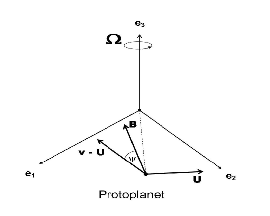
Figure 1: This illustration shows the protoplanet viewed in a frame rotating with the angular velocity of the star $\Omega_{*}$ here $\equiv\Omega,$ the latter being located at the origin of a Cartesian coordinate system $({\bf e_{1}},{\bf e_{2}},{\bf e_{3}})$ defining the direction of the axes. The protoplanet moves in a circular orbit in the equatorial plane with velocity ${\bf U}.$ The field line passing through its location points out of the plane ultimately reaching the star. In this frame the gas moves along field lines with velocity ${\bf v}$ and the line pointing in the direction of the relative velocity ${\bf v-U}$ makes an angle $\psi$ with that pointing in the direction of ${\bf B},$ or equivalently ${\bf V_{A}},$ which also gives the direction of the $z$ axis for the local frame in which the calculation is done. In that frame ${\bf v-U}$ lies in the $(x,z)$ plane.

On the basis of the above discussion, we here adopt the assumption that the protoplanet magnetosphere interaction is localised in the vicinity of the protoplanet and that the associated characteristic time scale is significantly shorter than the orbital period. Accordingly we adopt a local frame that can be taken to be a non rotating local Cartesian coordinate system with origin instantaneously at the centre of mass of the protoplanet and moving with a constant velocity equal to that of the rotational velocity the star would have if it extended to the radial location of the protoplanet (if one uses a local frame fixed in the original rotating frame and then neglects $\Omega_{*}$ in the equations of motion the same results are obtained). The response to the protoplanet is readily calculable and leads to a confirmation of the conclusion that the changes induced in the orbit are associated with wave energy fluxes propagating away from the protoplanet. Furthermore when such waves are absent, such as when the relative speed is below all possible wave speeds, there is no energy change induced on the orbit.

3.3 Linear Analysis

The effect of a perturbing protoplanet of mass $M_{p}$ at position vector ${\bf r}={\bf r}_{orb}$ is to produce an Eulerian perturbation to the gravitational potential $\Phi^{\prime}=-GM_{p}/\sqrt{|{\bf r}-{\bf r}_{orb}|^{2}+b^{2}},$ where $b$ is a softening parameter which can be specified to ensure $\Phi^{\prime}$ remains finite. An appropriate value is expected to be of the order of the radius of the planet.

In the original rotating frame, the Lagrangian displacement $\xi$ induced by by this perturbing potential satisfies the equation (see eg. Frieman & Rotenberg 1960; Lynden-Bell & Ostriker 1967)

$${D^{2}\mbox{\boldmath{$\xi$}}\over Dt^{2}}+2\Omega_{*}{\hat{\bf e_{3}}}\times{D\mbox{\boldmath{$\xi$}}\over Dt}=F(\mbox{\boldmath{$\xi$}}),$$ (7)

where the convective derivative operator

$${D\over Dt}\equiv{\partial\over\partial t}+{\bf v}\cdot\nabla$$ (8)

and the Lagrangian variation of the force per unit mass is $F(\mbox{\boldmath{$\xi$}})={\bf f}^{\prime}+\mbox{\boldmath{$\xi$}}\cdot\nabla{\bf f},$ with

$${\bf f^{\prime}}=-{{\nabla P^{\prime}}\over\rho}+{\rho^{\prime}\over\rho^{2}}\left(\nabla P-{(\nabla\times{\bf B})\times{\bf B}\over 4\pi}\right)\hskip 28.45274pt$$

$$\hskip 42.67912pt+{(\nabla\times{\bf B^{\prime}})\times{\bf B}\over 4\pi\rho}+{(\nabla\times{\bf B})\times{\bf B^{\prime}}\over 4\pi\rho}-\nabla\Phi^{\prime}.$$ (9)

The Eulerian perturbations to the magnetic field and density are given by

$${\bf B}^{\prime}=\nabla\times(\mbox{\boldmath{$\xi$}}\times{\bf B}),$$ (10)

and

$$\rho^{\prime}=-\nabla\cdot(\rho\mbox{\boldmath{$\xi$}}),$$ (11)

respectively. For an isothermal equation of state the Eulerian pressure perturbation $P^{\prime}=\rho^{\prime}c^{2}.$ Equations (7 - 11) thus provide a complete system for determining the Lagrangian displacement $\mbox{\boldmath{$\xi$}}.$

We make the usual local approximation that the steady state variables $\rho,$ $\Phi$ and $P$ as well as ${\bf v}$ and ${\bf B}$ can be taken to be constant. In the local frame ( see Figure 1) the velocity of the protoplanet is taken to be ${\bf U}$ and we may use equations (7 - 11) with $\Omega_{*}=0.$. Equation (7) then gives

$$\left({\partial\over\partial t}+{\bf v}\cdot\nabla\right)^{2}\mbox{\boldmath{$\xi$}}=-{{\nabla P^{\prime}}\over\rho}-\nabla\Phi^{\prime}+{(\nabla\times{\bf B^{\prime}})\times{\bf B}\over 4\pi\rho},$$ (12)

which together with equations (10), (11) and $P^{\prime}=-\rho^{\prime}c^{2}$ enable the Lagrangian displacement induced by the perturbing potential $\Phi^{\prime}$ to be calculated.

3.3.1 Fourier Transform of the Potential

For this local model, we set the softening parameter $b=0,$ so that in the local coordinates, the perturbing potential may be written $\Phi^{\prime}=-GM_{p}/|{\bf r}-{\bf U}t|,$ with ${\bf r}$ denoting the position vector. To solve (12) we take Fourier transforms of the perturbations. Thus for a general perturbation quantity $Q,$

$$Q=\int\exp(i{\bf k}\cdot{\bf r})Q_{\bf k}({\bf k})d^{3}{\bf k},$$ (13)

with the Fourier transform

$$Q_{\bf k}={1\over(2\pi)^{3}}\int\exp(-i{\bf k}\cdot{\bf r})Q({\bf r})d^{3}{\bf r}.$$ (14)

The wavenumber ${\bf k}=(k_{x},k_{y},k_{z})$ and the integrals are taken over all coordinate and wavenumber space. For the perturbing potential $\Phi^{\prime},$ one readily finds that

$$\Phi^{\prime}_{\bf k}=-{GM_{p}\over 2\pi^{2}|{\bf k}|^{2}}\exp(-i{\bf k}\cdot{\bf U}t).$$ (15)

3.3.2 Calculation of the Fourier Transform of the Displacement

After taking the Fourier transforms of equation (12) and equation (10) and noting that $P^{\prime}_{\bf k}=\rho^{\prime}_{\bf k}c^{2}=-\rho c^{2}\mbox{\boldmath{$\xi$}}_{\bf k}\cdot{\bf k},$ one obtains a set of linear algebraic equations for the determination of the components of $\mbox{\boldmath{$\xi$}}_{\bf k}$ in terms of $\Phi^{\prime}_{\bf k}.$ The scalar quantity $\mbox{\boldmath{$\xi$}}_{\bf k}\cdot{\bf k},$ is readily found after straightforward algebra to be given by

$$\mbox{\boldmath{$\xi$}}_{\bf k}\cdot{\bf k}={i\Phi^{\prime}_{\bf k}{\bf k}^{2}(\nu^{2}-({\bf k\cdot V_{A}})^{2})\over(\nu^{4}-(c^{2}+V_{A}^{2})\nu^{2}{\bf k}^{2}+({\bf k\cdot V_{A}})^{2}c^{2}{\bf k}^{2})},$$ (16)

where $\nu=({\bf k\cdot(v-U)})$ and ${\bf V_{A}}={\bf B}/\sqrt{4\pi\rho}$ denotes a vector, with magnitude equal to the Alfvèn speed, and the direction of ${\bf B}.$ We set $V_{A}=|{\bf V_{A}}|.$

The gravitational force acting on the protoplanet as a result of the perturbation of the magnetosphere can then be found using

$${\bf F_{orb}}=\int\rho^{\prime}\nabla\Phi^{\prime}d^{3}{\bf r}.$$ (17)

We evaluate the rate of change of orbital energy that would be viewed in the fluid rest frame. In that frame the drag force would be zero if ${\bf v}={\bf U}$ and consequently the rate of change of orbital energy would be zero. Otherwise it is given by

$${dE_{orb}\over dt}={\bf(U-v)\cdot F_{orb}}\ \ {\rm or}$$ (18)

$${dE_{orb}\over dt}=-(2\pi)^{3}Re\int\rho(\mbox{\boldmath{$\xi$}}_{\bf k}\cdot{\bf k})({\bf k\cdot(U-v)})\Phi^{\prime*}_{\bf k}d^{3}{\bf k}.$$ (19)

Here $Re$ indicates that the real part of the integral is to be taken.

In evaluating equation (19) we note that if there were no singularities in the expression for $\mbox{\boldmath{$\xi$}}_{\bf k}\cdot{\bf k}$ given by equation (16) we would have no energy exchange or ${dE_{orb}/dt}=0.$ Thus in order to obtain ${dE_{orb}/dt}\neq 0,$ there should be singularities in $\mbox{\boldmath{$\xi$}}_{\bf k}\cdot{\bf k}.$ In fact singularities in the form of simple poles occur when the denominator on the right hand side of equation (16) vanishes or when

$$\nu^{4}-(c^{2}+V_{A}^{2})\nu^{2}{\bf k}^{2}+({\bf k\cdot V_{A}})^{2}c^{2}{\bf k}^{2}=0.$$ (20)

This quartic gives four roots for $\nu$ given by $\nu=\pm r_{1,2}|{\bf k}|,$ where $r_{1}^{2}=(c^{2}+V_{A}^{2})/2+\sqrt{(c^{2}+V_{A}^{2})^{2}/4-({\bf{\hat{k}}\cdot V_{A}})^{2}c^{2}}$ and $r_{2}^{2}=(c^{2}+V_{A}^{2})/2-\sqrt{(c^{2}+V_{A}^{2})^{2}/4-({\bf{\hat{k}}\cdot V_{A}})^{2}c^{2}},$ with ${\bf{\hat{k}}}={\bf k}/|{\bf k}|.$

The roots corresponding to $r_{1}$ and $r_{2},$ which without loss of generality are taken to be positive, correspond to fast and slow magnetosonic waves respectively which propagate with angular frequency $\nu={\bf k\cdot(v-U)}.$ When any such waves can be present, there is the possibility of an induced change of orbital energy. This is entirely consistent with the fact, noted in section 3.4.1 below that the rate of change of orbital energy has to be associated with a conserved energy flux propagating away from the protoplanet. In the local problem considered here, this flux can be carried in either fast or slow magnetosonic waves. We also comment that in order to produce orbital energy changes, as is apparent from equation (17), the waves have to be compressive or associated with density perturbations, thus incompressible Alfvén waves are ineffective..

The singularities in $\mbox{\boldmath{$\xi$}}_{\bf k}\cdot{\bf k}$ given by (16) can be dealt with by writing the denominator as a product of factors of the form $({\tilde{\nu}}\pm r_{i}),$ for $(i=1,2)$ ${\tilde{\nu}}=\nu/|{\bf k}|$ and then handling the inverse of each these by using the well known Landau prescription, thus

$${1\over({\tilde{\nu}}\pm r_{i})}\rightarrow P\left({1\over({\tilde{\nu}}\pm r_{i})}\right)+\pi i\delta({\tilde{\nu}}\pm r_{i}).$$ (21)

Here $P$ denotes that the principal value is to be taken on integration and $\delta$ is Dirac’s $\delta$ function. This prescription results from adding an infinitesimally small negative imaginary part to ${\tilde{\nu}},$ which can be regarded as ensuring that the perturbing potential vanishes at $t=-\infty$ thus imposing causality. Using the Landau prescription and noting that roots of opposite sign give equivalent contributions, we can find the rate of change of orbital energy using equation (19) in the form

$${dE_{orb}\over dt}=-8(\pi)^{4}\rho\int{|\Phi^{\prime}_{\bf k}|^{2}{\tilde{\nu}}|{\bf k}|\over r_{1}r_{2}(r_{1}^{2}-r_{2}^{2})}\Lambda({\bf{\hat{k}}})d^{3}{\bf k},$$ (22)

where

$$\Lambda=r_{2}(r_{1}^{2}-({\bf{\hat{k}}\cdot V_{A}})^{2})\delta({\tilde{\nu}}-r_{1})$$

$$\hskip 71.13188pt-r_{1}(r_{2}^{2}-({\bf{\hat{k}}\cdot V_{A}})^{2})\delta({\tilde{\nu}}-r_{2})$$ (23)

To perform the above integral we first remark that because $r_{1},r_{2}$ and ${\tilde{\nu}}$ are functions only of the unit wavenumber vector, if polar coordinates in wavenumber space are adopted, the integrand easily factors into radial and angular parts, thus

$${dE_{orb}\over dt}=-2(GM_{p})^{2}\rho\int_{k_{min}}^{k_{max}}{dk\over k}\int{{\tilde{\nu}\Lambda({\bf{\hat{k}}})}\over r_{1}r_{2}(r_{1}^{2}-r_{2}^{2})}d\Omega,$$ (24)

where $d\Omega$ denotes integration over the solid angle in wavenumber space and $k_{max},k_{min}$ are the magnitudes of upper and lower wavenumber cut offs that necessarily have to be used in local calculations of gravitational interactions because of the long and short range form of the $1/r$ potential (see eg. Tremaine & Weinberg 1984 in the context of stellar dynamics and Papaloizou 2002 in the context of thin hydrodynamic disks). Physically $k_{max}^{-1}$ should be taken as the smallest effective length scale in the problem and $k_{min}^{-1}$ the largest. For a giant protoplanet in an inner magnetosphere, the ratio of the radius of the planet to a characteristic scale of the magnetosphere of $0.1AU,$ $\sim 10^{-2},$ accordingly one expects $k_{max}/k_{min}\sim 100.$

To perform the angular integral in equation(24), we specify the local frame such that the $z$ axis points along the direction of ${\bf B}$ and thus ${\bf V_{A}}$ and ${\bf v}.$ The direction of ${\bf v-U}$ is taken to be in the $(x,z)$ plane making an angle $\psi$ with the $z$ axis (see Figure 1). Using spherical polar angles $\theta,\phi$ to perform the integral over the solid angle, we note that because ${\bf{\hat{k}}\cdot V_{A}}/V_{A}=\cos\theta,$ $r_{1},r_{2}$ are functions only of $\theta.$ Given that ${\tilde{\nu}}\leavevmode\nobreak\ =\leavevmode\nobreak\ |{\bf v-U}|\leavevmode\nobreak\ (\cos\theta\cos\psi\leavevmode\nobreak\ +\leavevmode\nobreak\ \sin\theta\sin\psi\cos\phi\leavevmode\nobreak\ )\leavevmode\nobreak\ ,$ the delta functions readily enable the integration over $\phi$ and so we obtain an expression requiring only an integration over $\mu=\cos\theta$ in the form

$${dE_{orb}\over dt}=-{4\pi(GM_{p})^{2}\rho\over|{\bf v-U}|}\ln\left({k_{max}\over k_{min}}\right){\cal D},$$ (25)

where ${\cal D}=(I_{1,2}+I_{2,1})/\pi,$ with

$$I_{1,2}=\int_{D}{(r_{1}^{2}-V_{A}^{2}\mu^{2})d\mu\over(r_{1}^{2}-r_{2}^{2})\sqrt{(1-f_{1}^{2})\sin^{2}\psi-(\mu-f_{1}\cos\psi)^{2}}},$$ (26)

where $(f_{1},f_{2})=(r_{1},r_{2})/|{\bf v-U}|.$ In the above integral the domain of integration is either $(-1,1)$ or $(s_{1},s_{2}),$ where $s_{1}$ and $s_{2}$ are values of $\mu$ for which the square root in (26) is zero should they exist.

In general the dependence of $f_{1}$ and $f_{2}$ on $\mu$ through $r_{1}$ and $r_{2}$ makes the above integral intractable. However, it can be found in the limit of low $c/V_{A}$ that we consider here. Then $r_{1}=V_{A},$ and $r_{2}=c\mu.$

We first note that In the super Alfvénic case where both $f_{1}$ and $f_{2}$ are very small, one obtains ${\cal D}=1.$ This case of course applies to the limit of zero wave propagation speeds which corresponds to the dynamical friction calculation of Chandrasekhar (1943) and it can also be derived from the calculation of the linear response of collisionless particles by Tremaine & Weinberg (1984). We obtain ${\cal D}\leq 1$ so that then this quantity measures the factor by which the dynamical friction is reduced when compared to the estimate of Chandrasekhar (1943).

To emphasise that this can be a large reduction, we note that in the sub Alfvénic case when both $f_{1}$ and $f_{2}$ exceed unity, there is no wavelike response or domain of integration for $(I_{1,2},I_{2,1})$ so that ${\cal D}=0.$

When $f_{1}$ is large but $f_{2}$ very small so that slow waves exist but fast waves do not, we have $I_{1,2}=0$ and $I_{2,1}=(\pi\sin^{2}\psi)/2$ so that ${\cal D}=(\sin^{2}\psi)/2.$

Thus in this case the rate of change of orbital energy depends on the orientation of the magnetic field, being zero when $\psi=0.$ In this limit ${\bf U},$ ${\bf v}$ and ${\bf B}$ are all parallel.

There is no dynamical friction in that case because deflection of a fluid element towards the protoplanet requires motion perpendicular to the magnetic field lines.

In contrast when $\psi=\pi/2$ deflection towards the protoplanet can occur with the motion remaining parallel to the field lines. Then the interaction is uninhibited.

Finally when $f_{1}<1$ and $f_{2}=0,$ so that both waves exist but the ratio of propagation speeds is large, we obtain

${\cal D}=1-f_{1}^{2}(\cos^{2}\psi-(\sin^{2}\psi)/2).$ In this case the most effective reduction of the dynamical friction occurs when $\psi=0,$ then ${\cal D}=1-f_{1}^{2}.$

3.4 General Scalings for the Response and Torque

3.4.1 Conservation of Wave Action and Angular Momentum Evolution

We point out that in the inviscid case considered here, it is possible to derive a conservation law from equations (7 - 11) in the form

$${\partial\rho_{A}\over\partial t}+\nabla\cdot({\rho_{A}}{\bf v}+{\bf F_{A}})={\bf S_{A}},$$ (27)

where in Cartesian coordinates with ${\bf r}=(x_{1},x_{2},x_{3}),$ ${\bf v}=(v_{1},v_{2},v_{3}),$ $Im$ denoting that the imaginary part is to be taken and using the summation convention

$$\rho_{A}=Im\left(\rho\mbox{\boldmath{$\xi$}}^{*}\cdot{\partial\mbox{\boldmath{$\xi$}}\over\partial t}+\rho\Omega_{*}\mbox{\boldmath{$\xi$}}^{*}\cdot({\bf{e_{3}}\times}\mbox{\boldmath{$\xi$}})-\mbox{\boldmath{$\xi$}}\cdot{\partial\left(\rho v_{j}\mbox{\boldmath{$\xi$}}^{*}\right)\over\partial x_{j}}\right),$$ (28)

$${\bf F_{A}}=Im\left({{\bf B^{\prime*}}{\bf\times(\mbox{\boldmath{$\xi$}}\times B)}\over 4\pi}+{\nabla\times{\bf B}\cdot(\mbox{\boldmath{$\xi$}}^{*}\times\mbox{\boldmath{$\xi$}}){\bf B}\over 8\pi}+P^{\prime}\mbox{\boldmath{$\xi$}}^{*}\right)$$ (29)

and

$${\bf S_{A}}=-Im\left(\rho\mbox{\boldmath{$\xi$}}^{*}\cdot\nabla\Phi^{\prime}\right).$$ (30)

This conservation law is written for a general complex forcing potential Here we apply it to the situation where the forcing can be written as the real part of a potential $Re\left(\Phi^{\prime}\right),$ where $\Phi^{\prime}=g_{m}({\bf r})\exp(im(\omega_{p}t-\varphi)),$ $g_{m}$ is a complex function of ${\bf r},$ $m$ the azimuthal mode number and $\omega_{p}$ is the pattern speed, being the difference between the angular velocity of the orbiting protoplanet and $\Omega_{*}.$ In this case, provided the forcing potential vanishes at the fluid boundaries, the rate of increase of the energy of the fluid is

$${dE_{fluid}\over dt}=\int Re(\rho^{\prime})Re\left({\partial\Phi^{\prime}\over\partial t}\right)d^{3}{\bf r}={m\omega_{p}\over 2}\int{\bf S_{A}}d^{3}{\bf r}.$$ (31)

The quantities $m\omega_{p}\rho_{A}/2,m\omega_{p}{\bf F_{A}}/2$ may be regarded as the energy density and the non advected energy flux associated with the forcing. In particular when the forcing source ${\bf S_{A}}$ is localised in space, the rate of change of orbital energy is associated with a conserved energy flux propagating away to large distances from the protoplanet. The total effect of the protoplanet is obtained by summing the independent contributions from different $m.$

When the unperturbed configuration is axisymmetric and the perturbing potential $\Phi^{\prime}$ depends on $\varphi$ and $t$ in the combination $\omega_{p}t-\varphi,$ the energy fluxes convert to fluxes of the angular momentum component along the symmetry axis by dividing by the pattern speed.

Then the total torque acting on the fluid can be written as ${\cal T}=dJ_{fluid}/dt=\omega_{p}^{-1}dE_{fluid}/dt.$ When, as for the situations considered here, the wave fluxes produce an energy and angular momentum loss from the system, the orbit decays or $dE_{orb}/dt=-dE_{fluid}/dt<0.$

We comment that the fact that the energy changes in the orbit can be measured through energy fluxes at distant boundaries generalises a corresponding result for hydrodynamic disk forcing (see Papaloizou & Terquem 2006) to the general MHD case. In particular if there are no excited waves or advected disturbances, there are no induced changes to the orbit.

3.4.2 Torque Scaling

The scaling of the rate of energy change given by equation (25), that was obtained from the local analysis, with the physical parameters of the problem can be obtained quite generally. The length scale appropriate to the magnetosphere and the orbit is expeced to be $r_{0}.$ The unit of time is $\Omega_{*}^{-1},$ and the pattern speed is expected to be $\omega_{p}\sim\Omega_{*},$ giving a characteristic relative velocity $r_{0}\Omega_{*}.$ This velocity would be expected to be characteristic of both the flow velocity along field lines and the relative velocity between the orbiting protoplanet and the magnetosphere. For a characteristic density in the neighbourhood of the protoplanet, $\rho,$ we find natural scalings from equations (7 - 11) and (31) for the response displacement and torque such that $\mbox{\boldmath{$\xi$}}\propto r_{0}M_{p}/M_{*}$ and ${\cal T}\propto\rho(GM_{p})^{2}/(\Omega_{*}^{2}r_{0}).$ Thus we write

$${\cal T}={-1\over\omega_{p}}{dE_{orb}\over dt}=f\rho(GM_{p})^{2}/(\Omega_{*}^{2}r_{0}),$$ (32)

where $f$ includes dependence on softening or the small scale cut off as well as the existence of propagating waves. This is equivalent to quation (25) if $f=4\pi r_{0}\Omega_{*}^{2}\ln\left({k_{max}/k_{min}}\right){\cal D}/(|{\bf v-U}|\omega_{p})$

4 Discussion

4.1 Orbital Evolution Timescale

From equation (32) a characteristic rate of evolution of protoplanet in circular orbit at radius $r_{orb}$ can be estimated from

$$t_{orb}^{-1}=\left|{d{E_{orb}/dt}\over E_{orb}}\right|\sim{2\rho G^{2}M_{p}r_{orb}\over\Omega_{*}^{3}r_{0}^{4}}\left(\left({r_{0}\over r_{orb}}\right)^{3/2}-1\right).$$ (33)

For the magnetically dominated region (see eg. Bouvier et al. 2006) we set $\rho={\dot{M}}/(4\pi r_{0}^{3}\Omega_{*}).$ Then for $M_{*}=1M_{\odot},M_{p}=10^{-3}M_{*},r_{orb}=0.5r_{0}$ giving a location slightly interior to the 2:1 commensurability with $\Omega_{*},$ and a characteristic accretion rate for a protostellar disk ${\dot{M}}=3\times 10^{-8}M_{\odot}y^{-1}$ ( e.g. Muzerolle et al. 2003 ), we obtain $t_{orb}\sim 2\times 10^{11}y.$ Thus the expected evolution of such a protoplanet orbit is expected to be very small over a characteristic protostellar disk lifetime $\sim 10^{7}y.$ Note too that this result is not changed if the orbital decay rate is enhanced by a factor $f\sim 50,$ corresponding to use of equation (25) with ${\cal D}=1$ corresponding to effective wave propagation, $|{\bf v-U}|=(r_{0}\Omega_{*})/2$ and $k_{max}/k_{min}\sim 100.$ It also indicates that no additional mechanism, such as special torques acting near the inner disk edge (Masset et al. 2006) is needed to halt the inward migration of proto giant planets.

4.1.1 Protoplanet Accretion

It may also be argued that the expected accretion onto the protoplanet is negligible while it is inside the magnetosphere. In order that accretion can take place an amount of energy comparable to the orbital binding energy must be dissipated in order for material to become bound to the protoplanet. Thus an estimate of the accretion rate onto the protoplanet is given by

$${\dot{M}_{p}}\sim M_{p}\left|{1\over E_{orb}}{dE_{orb}\over dt}\right|,$$ (34)

which implies that the accretion time scale is the same as that for orbital evolution.

4.1.2 Other Effects

We here consider other effects that may lead to orbital decay of the protoplanet. First we derive an effective drag coefficient characterising the dynamical friction acting through the gravitational torques calculated above.

To do this we write

$${dE_{orb}\over dt}=-{1\over 2}C_{D}\pi R_{p}^{2}\rho|{\bf U}-{\bf v}|({\bf U}-{\bf v})\cdot{\bf U}$$ (35)

( Landau & Lifshitz 1993), where the expression is applied locally and $C_{D}$ is the drag coefficient. f Adopting $r_{0}/R_{p}=200,$ we find that the larger estimate of $t_{orb}$ given above corresponds to $C_{D}\sim 0.1$ while the smaller estimate corresponds to $C_{D}\sim 5.$ These results imply that the orbital decay rate is, to within an order of magnitude or so, comparable to the non gravitational effects arising from the protoplanet acting as an obstacle to the flow. This is in contrast to the situation that occurs for protoplanets in circular orbits in a thin disk (Lin & Papaloizou 1993).

4.1.3 Magnetic Coupling with the Central Star

Orbital energy decay can also result from the direct interaction of a conducting protoplanet with the stellar magnetic field when this varies around the orbit. When the stellar magnetic field is non axisymmetric and the protoplanet has a non zero resistivity , there will be periodic flux penetration and dissipation leading to an orbital energy loss. In the discussion below we neglect any internal protoplanetary magnetic field.

The rate of change of energy can be estimated to be (see e.g. Joss, Katz & Rappaport 1979 for a discussion of magnetic binary systems)

$${dE_{orb}\over dt}=-{3\over 8}R_{p}^{2}B_{||}^{2}\Delta R_{p}(\omega_{p}-v_{\varphi}/r),$$ (36)

where $\Delta R_{P}=\sqrt{\eta/(\omega_{p}-v_{\varphi}/r)}$ is a measure of the depth of external flux penetration per relative orbit, with $v_{\varphi}$ being the azimuthal component of the gas velocity, $B_{||}$ is a typical component of ${\bf B}$ parallel to the surface of the protoplanet, which we shall take to be $|{\bf B}|$ and $\eta$ is its magnetic diffusivity. We may also write

$${dE_{orb}\over dt}=-{3\pi\over 2}\rho V_{A}^{3}R_{p}^{2}{\Delta R_{p}(\omega_{p}-v_{\varphi}/r)\over V_{A}},$$ (37)

which leads to an effective drag coefficient given by

$$C_{D}={3V_{A}^{2}r(\omega_{p}-v_{\varphi}/r)\over||{\bf U}-{\bf v}|({\bf U}-{\bf v})\cdot{\bf U}|}\left({R_{p}\over r}\right)\left({\Delta R_{p}\over R_{p}}\right).$$ (38)

Although the flow is sub Alfvénic, the above is of order unity apart from the two factors in brackets. Of these $R_{p}/r\sim 10^{-2}$ and the last factor which represents the ratio of the skin depth to radius is also small. For example from Zhang, Jones & Chen (1996) the magnetic diffusivity of Jupiter can be estimated to be $\eta=3\times 10^{3}cm^{2}s^{-1}.$ For a relative orbital period of $10\ {\rm days},$ this leads to $\Delta R_{p}/R_{p}\sim 10^{-5}$ and the effective $C_{D}\sim 10^{-6}.$ Thus the effect of this type of magnetic interaction with the central star is not likely to be significant.

4.2 Conclusions

In this paper we performed a local calculation of the protoplanet magnetosphere interaction derived. The existence of propagating waves was necessary for there to be a non zero energy exchange rate. This is also expected from very general considerations of energy and wave action conservation. For high relative speeds between the gas and protoplanet, the interaction was found to be identical to that obtained from the dynamical friction formalism of Chandrasekhar (1943). But when, as expected here, the relative flow speed is below the fast magnetosonic speed but exceeds the slow magnetosonic speed, the interaction strength was found to be reduced, especially when the relative velocity between gas and protoplanet was parallel or nearly parallel to the magnetic field. The inhibition of the ability of the protoplanet to disturb the flow in such cases would also be expected to apply to the gas accretion rate onto it.

For parameters expected for protoplanetary disks our calculation indicates negligible orbital evolution for protoplanets interior to magnetospheric cavities through which accretion is taking place during expected protoplanetary disk lifetimes. This is the situation when the protoplanets are far enough away from the inner disk edge so that interaction with the disk is negligible and accordingly it is not necessary to invoke special torques associated with the disk edge to halt or reverse migration. In this regard we comment that although there have been, of necessity, many simplifying assumptions made in order to carry out the analysis presented here, the expected protoplanet orbital evolution in the magnetosphere fails to be significant by a wide margin.

References

- Armitage Clarke (1996) Armitage, P.J., Clarke, C.J., 1996, MNRAS, 280, 458
- Bouvier (2006) Bouvier, J., Alencar, S.H.P., Harries, T.J., Johns-Krull, C.M., Romanova, M. M., 2006, Protostars and Planets V ed B. Reipurth, D. Jewitt and K. Keil (Tucson: University of Arizona Press)in press
- Cameron & Campbell (1993) Cameron, A.C., Campbell, C.G., 1993, A&A, 274, 309
- Chandrasekhar (1943) Chandrasekhar, S., 1943 ApJ, 97, 251
- Frieman & Rotenberg (1960) Frieman, E., Rotenberg, M., 1960, Rev. Mod. Phys., 32, 898
- Ghosh & Lamb (1978) Ghosh, P., Lamb, F.K., 1978 ApJ, 223, L83
- Goldreich & Tremaine (1980) Goldreich, P., Tremaine, S., 1980, ApJ, 241, 425
- Hoyle Lyttleton (1939) Hoyle, F., Lyttleton, R.A. 1939, Proc. Cam. Phil. Soc., 35, 405
- JohnsKrull et al (1999) Johns-Krull, C.M., Valenti, J.A., Hatzes, A.P., Kanaan, A., 1999, ApJ, 510, L39
- Joss et al (1979) Joss, P.C., Katz, J.I., Rappaport, S.A., 1979, ApJ, 230, 176
- Landau (1993) Landau, L.D., Lifshitz, E.M. 1993, Fluid Mechanics (Oxford University Press)
- Lin Bodenheimer & Richardson (1996) Lin, D.N.C., Bodenheimer, P., Richardson, D.C. 1996, Nature, 380, 606
- Lin & Papaloizou (1993) Lin, D.N.C., Papaloizou, J.C.B., 1993 Protostars and Planets III ed E.H. Levy and J.I. Lunine (Tucson: University of Arizona Press) p 749
- Lynden-Bell & Ostriker (1967) Lynden-Bell, D., Ostriker, J.P., 1967, MNRAS, 136, 293
- Marcy et al. (1995) Marcy, G.W., Butler, R.P., 1995, 187th AAS Meeting BAAS vol 27 p 1379
- Marcy et al. (1998) Marcy, G.W., Butler, R.P., 1998, Annu. Rev. Astron. Astr., 36, 57
- Masset et al (2006) Masset, F., Morbidelli, A., Crida, A., Ferreira, J., 2006, ApJ, 642, 478
- Matt & Pudritz (2004) Matt, S., Pudritz, R.E., 2004, MNRAS, 356, 167
- Mayor (1995) Mayor, M., Queloz, D., 1995, Nature 378 355
- Menard (2003) Ménard, F., Bouvier, J., Dougados, C., Mel’nikov, S.Y., Grankin, K. N., 2003, A&A, , 409, 163
- McArthur et al. (2004) Muzerolle, J., Hillenbrand, L., Calvet, N., Brice o, C., Hartmann, L., 2003, ApJ, 592, 266
- Nelson et al. (2000) Nelson, R.P., Papaloizou, J.C.B., Masset, F., Kley, W., 2000, MNRAS, 318, 18
- Papaloizou (2002) Papaloizou, J.C.B., 2002, A&A, , 388, 615
- Papaloizou & Terquem (2006) Papaloizou, J.C.B., Terquem, C., 2006, Rep. Prog. Phys., 69, 119
- Pringle (1981) Pringle, J.E., 1981, ARA&A, , 19, 137
- Romanova (2004) Romanova, M.M., Ustyugova, G.V., Koldoba, A.V., Lovelace, R.V.E., 2004, ApJ, 610, 920
- Romanova (2006) Romanova, M.M., Lovelace, R.V.E., 2006, ApJ, 645, L73
- Ruffert (1996) Ruffert, M. 1996, A&A, , 311, 817
- Safier (1998) Safier, P.N., 1998, ApJ, 494, 336
- Tremaine & Weinberg (1984) Tremaine, S., Weinberg, M.D., 1984, MNRAS, 209, 729
- Zhang, Jones & Chen (1996) Zhang, K., Jones, C.A., Chen, D., 1996, EM&P 73, 221