Observational Constraints with Recent Data on the DGP Modified Gravity

Abstract

We study one of the simplest covariant modified-gravity models based on the Dvali-Gabadadze-Porrati (DGP) brane cosmology, a self-accelerating universe. In this model gravitational leakage into extra dimensions is responsible of late-time acceleration. We mainly focus on the effects of the model parameters on the geometry and the age of universe. Also we investigate the evolution of matter density perturbations in the modified gravity model, and obtain an analytical expression for the growth index, $f$. We show that increasing $\Omega_{r_{c}}$ leads to less growth of the density contrast $\delta$, and also decreases the growth index. We give a fitting formula for the growth index at the present time and indicate that dominant term in this expression verifies the well-known approximation relation $f\simeq\Omega_{m}^{\gamma}$. As the observational test, the new Supernova Type Ia (SNIa) Gold sample and Supernova Legacy Survey (SNLS) data, size of baryonic acoustic peak from Sloan Digital Sky Survey (SDSS), the position of the acoustic peak from the CMB observations and the Cluster Baryon Gas Mass Fraction (gas) are used to constrain the parameters of the DGP model. We also combine previous results with large scale structure formation (LSS) from the $2$dFGRS survey. Finally to check the consistency of the DGP model, we compare the age of old cosmological objects with age of universe in this model.
PACS numbers: 05.10.-a ,05.10.Gg, 05.40.-a, 98.80.Es, 98.70.Vc

1 Introduction

Recent Observations of type Ia supernova (SNIa) provides the main evidence for accelerating expansion of the Universe ris ; permul . Analysis of SNIa and the Cosmic Microwave Background radiation (CMB) observations indicates that about $70\%$ of the total energy of the Universe is made by the dark energy and the rest of it is the dark matter with a few percent of Baryonic matter bennett ; peri ; spe03 . The ”cosmological constant” is a possible explanation for the acceleration of the universe wein . This term in Einstein field equations can be regarded as a fluid with the equation of state of $w=-1$. However, there are two problems with the cosmological constant, namely the fine-tuning and the cosmic coincidence. In the framework of quantum field theory, the vacuum expectation value is $123$ order of magnitude larger than the observed value of $10^{-47}$ GeV⁴. The absence of a fundamental mechanism which sets the cosmological constant to zero or to a very small value is the cosmological constant problem. The second problem known as the cosmic coincidence, states that why are the energy densities of dark energy and dark matter nearly equal today?

There are various solutions for this problem as the decays cosmological constant models. A non-dissipative minimally coupled scalar field, the so-called Quintessence model can play the role of this time varying cosmological constant wet88 ; amen ; peb88 . The ratio of energy density of this field to the matter density in this model increases by the expansion of the universe and after a while dark energy becomes the dominant term of the energy-momentum tensor. One of the features of this model is the variation of equation of state during the expansion of the universe. Various Quintessence models like k-essence arm00 , tachyonic matter pad03 , Phantom cal02 ; cal03 and Chaplygin gas kam01 provide various equations of states for the dark energy cal03 ; kam01 ; wan00 ; per99 ; pag03 ; dor01 ; dor02 ; dor04 ; arb05 .

Another approach dealing with this problem is using the modified gravity by changing the Einstein-Hilbert action. Some of models as $1/R$ and logarithmic models provide an acceleration for the universe at the present time bar05 . In addition to the phenomenological modification of action, the brane cosmology also implies modification for the general relativity on a brane embedded in an extra dimension space. Some brane world models which produce the late time acceleration have been tested using many observational experiments such as local gravity Lue03 ; lue03 ; lue04 , Supernova Type Ia bar05 ; zong ; deff021 ; ane02 ; dab04 ; alm05 ; maartens1 ; saf , angular size of compact ratio sources alca02 , the age measurements of high redshift objects alca021 , the optical gravitational lensing surveys jain02 , the large scale structures mul03 , and the X-ray gas mass fraction in galaxy clusters zhu ; alca05 .

In some recent papers maartens1 ; Barger ; mf06 observational constraints have been obtained through the old data of Supernova Gold sample and its combination with CMB shift parameter and Baryon acoustic oscillation. Recently Guo et al. have put constraints on this model using recent SNIa data and Baryon acoustic oscillation zong . Song et al., Sawichi and Carroll have separately investigated the effect of DGP on the integrated Sachs-Wolfe and tested the validity of modified linear growth factor in the sub-horizon scale yong ; saw05 . In ref. yong linear growth of density contrast in this model has been reviewed but some of the interesting quantity as the growth index and its behavior versus redshift and its dependency to the model parameter is missed.

In this paper we examine the effects of DGP model on the geometrical parameters of the universe. On the other hand we use the observational results related to the background evolution. Since the structure formation in DGP is currently well understood on scales between a few percent of the Hubble scale and the scale radius of a typical dark matter halo maartens2 , we combine those results with the linear structure formation of large scale in the universe. Meanwhile we concentrate our attention to the effect of $\Omega_{r_{c}}$ and $\Omega_{m}$ as free parameters of the model on the density contrast and growth index evolution. We extend the simplest growth index analytic formula given for the flat $\Lambda$CDM f in the underlying modified gravity model. We organize this paper as follows: In Sec.2. DGP MODIFIED GRAVITY we introduce DGP model as a self-accelerating cosmology. Its free parameters and modified Friedman equation which governs on the background dynamics of the universe are also investigated. In Sec.2 we study the effect of this model on the comoving distance, comoving volume element, the variation of angular size by the redshiftalc79 . In Sec. 3 we put some constraints on the parameters of model by using the background evolution, such as new Gold sample and Legacy Survey of Supernova Type Ia data R04 , the position of the observed acoustic angular scale on the last scattering surface, CMB shift parameter, the baryonic oscillation length scale and baryon gas mass fraction for the range of redshift, $z\leq 1.0$. We study the linear structure formation in this model and compare the growth index with the observations from the $2-$degree Field Galaxy Redshift Survey ($2$dFGRS) data in Sec. 4. We also compare the age of the universe in this model with the age of old cosmological structures in Sec. 5. Sec.6 contains summary and conclusion of this work.

2. DGP MODIFIED GRAVITY

One of the simplest covariant modified-gravity models is based on the Dvali-Gabadadze-Porrati (DGP) brane-world model, as generalized to cosmology by Deffayet Dvali:2000rv . (It is worth noting that the original DGP model with a Minkowski brane was not introduced to explain acceleration – the generalization to a Friedman brane was subsequently found to be self-accelerating.) In this model, gravity leaks off the 4-dimensional brane universe into the 5-dimensional bulk spacetime at large scales. Ordinary matter is considered to be localized on the brane while gravity can propagate in the bulk. At small scales, gravity is effectively bound to the brane and 4D gravity is recovered to a good approximation. The action for the five-dimensional theory is:

$$S=\frac{1}{2\kappa_{5}^{2}}\int d^{5}x\sqrt{-g_{(5)}}R_{(5)}+\frac{1}{2\kappa_{4}^{2}}\int d^{4}x\sqrt{-g_{(4)}}R_{(4)}+S_{\rm matter}$$ (1)

where the subscripts $4$ and $5$ denote the quantities on the brane and in the bulk, respectively, $\kappa_{4}^{2}(\kappa_{5}^{2})$ is the inverse of four(five)-dimensional reduced Planck mass, and $S_{\rm matter}$ is the action for matter on the brane. The solution of DGP action in FRW metric provides a self-accelerating universe for the expanding phase of the universe. This model can be an alternative to the cosmological constant for describing the present acceleration of the universe. However, DGP model suffers from the ghost instability that was shown in ghost1 ; ghost2 though the boundary effective action formalism. On the other hand the existence of ghost is confirmed by explicit calculation of the spectrum of linear perturbations in the five-dimensional framework ghost3 . A solution for this problem is so-called cascading DGP model in which the unlike previous attempts, it is free of ghost instabilities. In this model the 4D propagator is regulated by embedding the 3-brane within a 4-brane with their own gravity terms induced by a flat 6D bulk ghost4 .

Coming back to the action (1), at moderate scales the induced gravity term is responsible for the recovery of 4-Dimensional Einstein gravity. The transition from 4D to 5D behavior is governed by a crossover scale $r_{c}$:

$$r_{c}\equiv\frac{\kappa_{5}^{2}}{2\kappa_{4}^{2}}.$$ (2)

In the weak-field gravitational field, potential behaves as $r^{-1}$ for $r\ll r_{c}$ and as $r^{-2}$ for $r\gg r_{c}$. At large scale gravity is five dimensional. The energy conservation equation remains the same as in general relativity, but the Friedman equation is modified:

$$\dot{\rho}+3H(\rho+p)=0\,,$$ (3)

$$H^{2}+{K\over a^{2}}\pm{1\over r_{c}}\sqrt{H^{2}+{K\over a^{2}}}={8\pi G\over 3}\rho$$ (4)

Two given sign in equation (4) correspond to the two branches of the cosmological evolution. The upper sing shows a de Sitter expansion of the universe, while the lower sign corresponds to the self-accelerating solution without the cosmological constant. So we infer the cosmological effects of the second branch of DGP model. Equations (3) and (4) imply (for the CDM case $p=0$)

$$\dot{H}-{K\over a^{2}}=-4\pi G\rho\left[1+{1\over\sqrt{1+32\pi Gr_{c}^{2}\rho/3}}\right]$$ (5)

Equation (4) shows that at early times, when $H^{2}+K/a^{2}\gg r_{c}^{-2}$, the general relativistic Friedman equation is recovered. By contrast, at late times in a CDM universe, with $\rho\propto a^{-3}\to 0$, we have

$$H\to H_{\infty}={1\over r_{c}}$$ (6)

Gravity leakage at late times initiates acceleration not due to any negative pressure field, but due to the weakening of gravity on the brane. Since $H_{0}>H_{\infty}$, in order to achieve self-acceleration at late times, we require

$$r_{c}>H_{0}^{-1}$$ (7)

and this is confirmed by fitting observations as discussed below.

In dimensionless form, the modified Friedman equation (4) is given by

$${H(z)^{2}\over H_{0}^{2}} = \left[\sqrt{\Omega_{m}(1+z)^{3}+\Omega_{r_{c}}}+\sqrt{\Omega_{r_{c}}}\right]^{2}$$ (8)

$$~{}~{}{}+\Omega_{K}(1+z)^{2}\,$$

where

$$\Omega_{K} = 1-\Omega_{m}-2\sqrt{\Omega_{r_{c}}}\left(\!\sqrt{\Omega_{r_{c}}}+\sqrt{\Omega_{r_{c}}+\Omega_{m}}\right)$$ (9)

$$= 1-\Omega_{tot}\!\!$$

$$\Omega_{r_{c}} = {1\over 4H_{0}^{2}r_{c}^{2}}\,.$$ (10)

From equation (5), the dimensionless acceleration is

$$q = {1\over H_{0}^{2}}{\ddot{a}\over a}=\left(\sqrt{\Omega_{m}(1+z)^{3}+\Omega_{r_{c}}}+\sqrt{\Omega_{r_{c}}}\right)\Biggl{[}\sqrt{\Omega_{r_{c}}}$$ (11)

$$~{}{}+{2\Omega_{r_{c}}-\Omega_{m}(1+z)^{3}\over 2\sqrt{\Omega_{m}(1+z)^{3}+\Omega_{r_{c}}}}\Biggr{]}$$

so that the redshift at which acceleration era is started is given by zhu

$$z_{q=0}=2\left({\Omega_{r_{c}}\over\Omega_{m}}\right)^{\frac{1}{3}}-1$$ (12)

Also equation (9) shows in the flat model:

$$\Omega_{r_{c}}={1\over 4}(1-\Omega_{m})^{2}$$ (13)

For the transition from negative to the positive acceleration at the present-time, equation (12) implies :

$$\Omega_{r_{c}}={\Omega_{m}\over 8}$$ (14)

Acceleration parameter for this model in terms of scale factor is shown in Figure 1. Increasing the value of $\Omega_{r_{c}}$ causes that universe entered in the acceleration phase at the earlier times. The lower panel of Figure 1 shows acceleration parameter for the flat $\Lambda$CDM model, obviously $\Omega_{r_{c}}$ has the same role as cosmological constant.

The modified Friedman equation in DGP may be reinterpreted from a standard viewpoint. We define the effective dark energy density $\rho_{eff}\equiv 3H/8\pi Gr_{c}$. Then the effective dark energy equation of state $w_{eff}\equiv p_{eff}/\rho_{eff}$ is given by $\dot{\rho}_{eff}+3H(1+w_{eff})\rho_{eff}=0$. Thus $\rho_{eff}$ and $w_{eff}$ give a standard general relativistic interpretation of DGP expansion history, i.e., they describe the equivalent general relativity dark energy model. For the flat case, $\Omega_{K}=0$, we find

$$w_{eff}(z)={\Omega_{m}-1-\sqrt{(1-\Omega_{m})^{2}+4\Omega_{m}(1+z)^{3}}\over 2\sqrt{(1-\Omega_{m})^{2}+4\Omega_{m}(1+z)^{3}}}\,,$$ (15)

which implies

$$w_{eff}(0)=-{1\over 1+\Omega_{m}}\,.$$ (16)

The DGP and $\Lambda$CDM models have the same number of parameters, with $r_{c}$ substituting $\Lambda$, therefore DGP model gives a very useful framework for comparing the $\Lambda$CDM general relativistic cosmology to a modified gravity alternative. Now an interesting question that arises is: ”can DGP model predict dynamics of universe?” or in another word, ”what values of the model parameter to be consistent with observational tests?”

In the forthcoming sections we will study the observational constraints on the model.

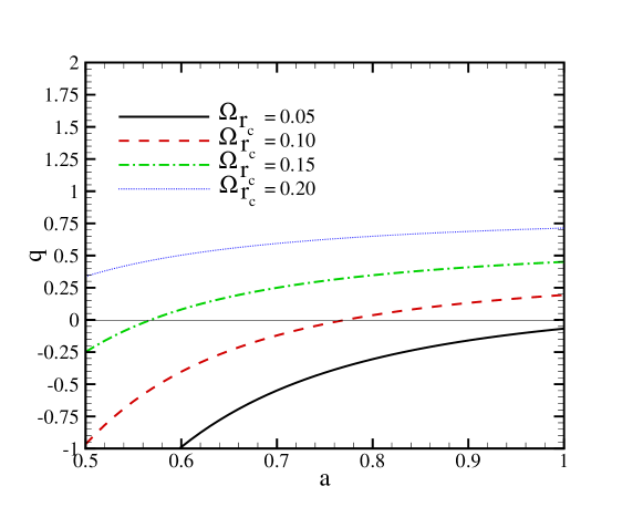
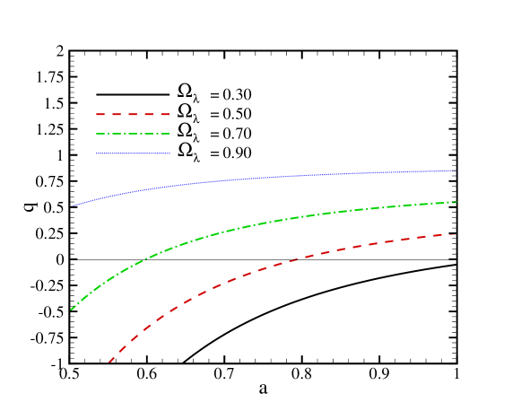
Figure 1: Upper panel shows acceleration parameter $(q=\ddot{a}/{H_{0}^{2}a})$ in the DGP model as a function of scale factor for various values of $\Omega_{r_{c}}$. Lower panel corresponds to the same function for the flat $\Lambda$CDM. We chose the flat universe.

2 The effect of DGP model on the geometrical parameters of universe

The cosmological observations are mainly affected by the background dynamics of universe. In this part we study the sensitivity of the geometrical parameters on the parameters of DGP model.

2.1 comoving distance

The radial comoving distance is one of the basic parameters in cosmology. For an object with the redshift of $z$, using the null geodesics in the FRW metric, the comoving distance is obtained as:

$$r(z;\Omega_{m},\Omega_{r_{c}}) = {1\over H_{0}\sqrt{|\Omega_{K}|}}\,{\cal F}\left(\sqrt{|\Omega_{K}|}\int_{0}^{z}\,{dz^{\prime}\over H(z^{\prime})/H_{0}}\right),$$

where

$${\cal F}(x) \equiv (x,\sin x,\sinh x)~{}for~{}K=(0,1,-1)\,.$$ (18)

and $H(z;\Omega_{m},\Omega_{r_{c}})$ is given by equation (8).

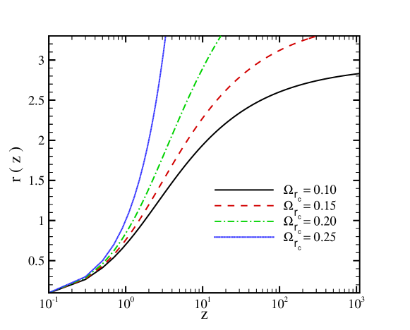
Figure 2: Comoving distance, $r(z;\Omega_{m},\Omega_{r_{c}})$ (in unit of $c/H_{0}$) as a function of redshift for various values of $\Omega_{r_{c}}$. We fixed $\Omega_{K}=0.0$.

By numerical integration of equation (2.1), the comoving distance in terms of redshift for different values of $\Omega_{r_{c}}$ is shown in Figure 2. Increasing the $\Omega_{r_{c}}$ results in a longer comoving distance. According to this behavior, by tuning the value of $\Omega_{r_{c}}$ we may explain the Supernova Type Ia observations.

2.2 Angular Size

The apparent angular size of an object located at the cosmological distance is another important parameter that can be affected by the cosmological model during the history of the universe. An object with the physical size of $D$ is related to the apparent angular size of $\theta$ by:

$$D=d_{A}\theta$$ (19)

where $d_{A}=r(z;\Omega_{m},\Omega_{r_{c}})/(1+z)$ is the angular diameter distance. The main applications of equation (19) is on the measurement of the apparent angular size of acoustic peak on CMB and baryonic acoustic peak at the high and low redshifts, respectively. By measuring the angular size of an object in different redshifts (the so-called Alcock-Paczynski test) it is possible to probe the validity of modified gravity models alc79 . The variation of apparent angular size $\Delta\theta$ in terms of $\Delta z$ is given by:

$${\Delta z\over\Delta\theta}=H(z;\Omega_{m},\Omega_{r_{c}})r(z;\Omega_{m},\Omega_{r_{c}})$$ (20)

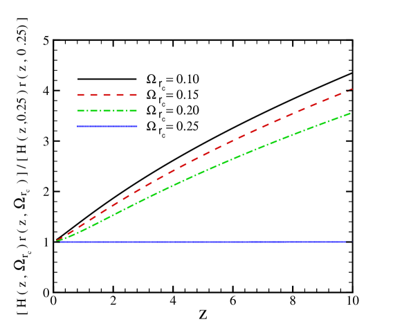
Figure 3: Alcock-Paczynski test comparing $\Delta z/{\Delta\theta}$ as a function of redshift for four different $\Omega_{r_{c}}$ normalized to the case with $\Omega_{m}=0$ and $\Omega_{r_{c}}=0.25$ (flat universe $\Omega_{K}=0$). It must be pointed out that for other values of $\Omega_{r_{c}}$ we also assumed $\Omega_{K}=0.0$.

Figure 3 shows $\Delta z/\Delta\theta$ in terms of redshift, normalized to the case with $\Omega_{m}=0.0$ and flat universe $\Omega_{K}=0.0$. The advantage of Alcock-Paczynski test is that it is independent of standard candles and knowing a standard ruler such as the size of baryonic acoustic peak one can use it to constrain the modified gravity model.

2.3 Comoving Volume Element

The comoving volume element is another geometrical parameter which is used in number-count tests such as lensed quasars, galaxies, or clusters of galaxies. The comoving volume element in terms of comoving distance and Hubble parameter is given by:

$$f(z;\Omega_{m},\Omega_{r_{c}})\equiv{dV\over dzd\Omega}=r^{2}(z;\Omega_{m},\Omega_{r_{c}})/H(z;\Omega_{m},\Omega_{r_{c}}).$$ (21)

According to Figure 4, the comoving volume element becomes large for larger value of $\Omega_{r_{c}}$ in the flat universe.

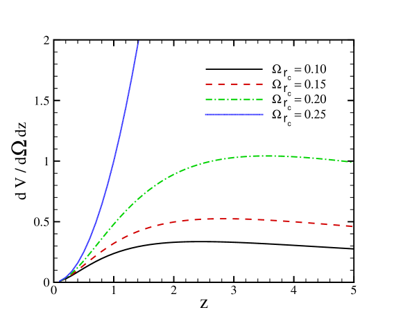
Figure 4: The comoving volume element in terms of redshift for various $\Omega_{r_{c}}$ exponent. Increasing $\Omega_{r_{c}}$ shifts the position of the maximum value of volume element to lower redshifts. We fixed $\Omega_{K}=0.0$

.

3 Observational Constraints From the Background Evolution

In this section we compare the SNIa Gold sample released from more recent observations new which have lower systematic errors than the former Gold sample data set. This new catalog contains $156$ Supernova type Ia. On the other hand we also take into account $116$ supernova Legacy Survey data which seems to be more consistent with WMAP observation as another SNIa observations to examine DGP model. To make the acceptance interval of model free parameters more confined, we use the location of acoustic peak of temperature fluctuations from WMAP observation, the location of baryonic acoustic oscillation peak from the SDSS and baryon gas mass fraction in the cluster for $26$ samples at redshifts less than $1$ allen04 . The Supernova Type Ia experiments provided the main evidence of the existence of dark energy. Since 1995 two teams of the High-Z Supernova Search and the Supernova Cosmology Project have discovered several type Ia supernovas at the high redshifts per99 ; Schmidt . Recently Riess et al.(2004) announced the discovery of $16$ type Ia supernova with the Hubble Space Telescope. This new sample includes $6$ of the $7$ most distant ($z>1.25$) type Ia supernovas. They determined the luminosity distance of these supernovas and with the previously reported algorithms, obtained a uniform $156$ Gold sample of type Ia supernovas as a new data set with lower systematic errors than former Gold sample data R04 ; Tonry ; bar04 . At the beginning we compare the predictions of the DGP model with the recent SNIa Gold sample new . The observations of supernova measure essentially the apparent magnitude $m$ including reddening, K correction, etc, which are related to the (dimensionless) luminosity distance, $D_{L}$, of an object at redshift $z$ through:

$$m={\mathcal{M}}+5\log{D_{L}(z;\Omega_{m},\Omega_{r_{c}})},$$ (22)

where

$$D_{L}(z;\Omega_{m},\Omega_{r_{c}}) = {(1+z)\over\sqrt{|\Omega_{K}|}}\,{\cal F}\left(\sqrt{|\Omega_{K}|}\int_{0}^{z}\,{dz^{\prime}H_{0}\over H(z^{\prime})}\right).$$ (23)

Also

$$\mathcal{M} = M+5\log{\left(\frac{c/H_{0}}{1\quad Mpc}\right)}+25.$$ (24)

where $M$ is the absolute magnitude. The distance modulus, $\mu$, is defined as:

$$\mu\equiv m-M = 5\log{D_{L}(z;\Omega_{m},\Omega_{r_{c}})}$$ (25)

$$\quad+5\log{\left(\frac{c/H_{0}}{1\quad Mpc}\right)}+25,$$

or

$$\mu = 5\log{D_{L}(z;\Omega_{m},\Omega_{r_{c}})}+\bar{M}$$ (26)

In order to compare the theoretical results with the observational data, we must compute the distance modulus, as given by equation (25). For this purpose,the first step is to compute the quality of the fitting through the least squared fitting quantity $\chi^{2}$ defined by:

$$\chi^{2}(\bar{M},\Omega_{m},\Omega_{r_{c}}) = \sum_{i}\frac{[\mu_{obs}(z_{i})-\mu_{th}(z_{i};\Omega_{m},\Omega_{r_{c}},\bar{M})]^{2}}{\sigma_{i}^{2}},$$

where $\sigma_{i}$ is the observational uncertainty in the distance modulus. To constrain the parameters of model, we use the Likelihood statistical analysis:

$${\cal L}(\bar{M},\Omega_{m},\Omega_{r_{c}})={\mathcal{N}}e^{-\chi^{2}(\bar{M},\Omega_{m},\Omega_{r_{c}})/2}$$ (28)

where ${\mathcal{N}}$ is a normalization factor. The parameter $\bar{M}$ is a nuisance parameter and should be marginalized (integrated out) leading to a new $\bar{\chi}^{2}$ defined as:

$$\bar{\chi}^{2}=-2\ln\int_{-\infty}^{+\infty}{\cal L}(\bar{M},\Omega_{m},\Omega_{r_{c}})d\bar{M}$$ (29)

Using equations (3), (28) and (29), we find:

$$\bar{\chi}^{2}(\Omega_{m},\Omega_{r_{c}}) = \chi^{2}(\bar{M}=0,\Omega_{m},\Omega_{r_{c}})-\frac{B(\Omega_{m},\Omega_{r_{c}})^{2}}{C}$$ (30)

$$+\ln(C/2\pi)$$

where

$$B(\Omega_{m},\Omega_{r_{c}})=\sum_{i}\frac{[\mu_{obs}(z_{i})-\mu_{th}(z_{i};\Omega_{m},\Omega_{r_{c}},\bar{M}=0)]}{\sigma_{i}^{2}},$$ (31)

$$C=\sum_{i}\frac{1}{\sigma_{i}^{2}},$$ (32)

Equivalent to marginalization is the minimization with respect to $\bar{M}$. One can show that $\chi^{2}$ can be expanded in $\bar{M}$ as Nesseris04 :

$$\chi^{2}(\Omega_{m},\Omega_{r_{c}})=\chi^{2}(\bar{M}=0,\Omega_{m},\Omega_{r_{c}})-2\bar{M}B+\bar{M}^{2}C$$ (33)

which has a minimum for $\bar{M}=B/C$:

$$\chi^{2}_{\rm SNIa}(\Omega_{m},\Omega_{r_{c}})=\chi^{2}(\bar{M}=0,\Omega_{m},\Omega_{r_{c}})-\frac{B(\Omega_{m},\Omega_{r_{c}})^{2}}{C}$$ (34)

Using equation (34) we can find the best fit values of model parameters as the values that minimize $\chi^{2}(\Omega_{m},\Omega_{r_{c}})$. For the Likelihood analysis we use some weak priors for the model parameters indicated in Table 1.

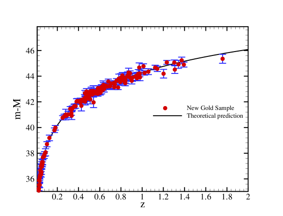
Figure 5: Distance modulus of the SNIa new Gold sample in terms of redshift. Solid line shows the best fit values with the corresponding parameters of $h=0.64$, $\Omega_{m}=0.36^{+0.07}_{-0.06}$, $\Omega_{r_{c}}=0.23_{-0.04}^{+0.04}$ in $1\sigma$ level of confidence with $\chi^{2}_{min}/N_{d.o.f}=0.91$ for DGP model.

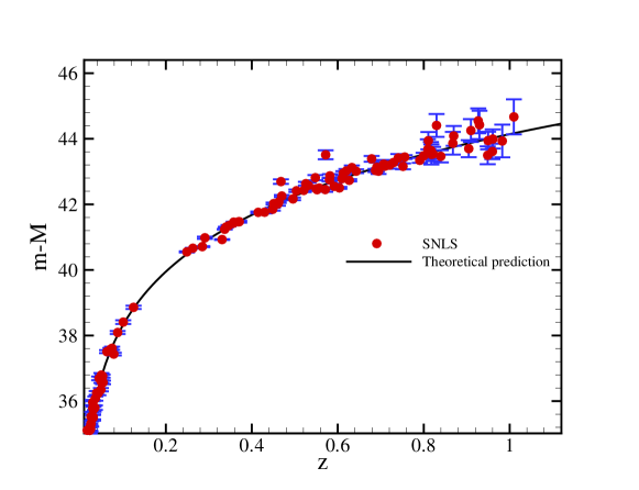
Figure 6: Distance modulus of the SNLS supernova data in terms of redshift. Solid line shows the best fit values with the corresponding parameters of $h=0.70$, $\Omega_{m}=0.13^{+0.06}_{-0.06}$, $\Omega_{r_{c}}=0.14_{-0.03}^{+0.03}$ in $1\sigma$ level of confidence with $\chi^{2}_{min}/N_{d.o.f}=0.85$ for DGP model.

Table 1: Priors on the parameter space, used in the likelihood analysis.

Parameter	Prior
$\Omega_{tot}$	-	Free
$\Omega_{m}$	$0.00-1.00$	Top hat
$\Omega_{r_{c}}$	$0.00-1.00$	Top hat
$\Omega_{b}h^{2}$	$0.020\pm 0.005$	Top hat (BBN)
$h$	$-$

The best values for the parameters of the model are: $\Omega_{m}=0.36^{+0.07}_{-0.06}$, $\Omega_{r_{c}}=0.23_{-0.04}^{+0.04}$ and $\Omega_{K}=-0.56^{+0.20}_{-0.20}$ with $\chi^{2}_{min}/N_{d.o.f}=0.91$ at $1\sigma$ level of confidence. The corresponding value for the Hubble parameter at the minimized $\chi^{2}$ is $h=0.64$ and since we have already marginalized over this parameter we do not assign an error bar for it. The best fit values for the parameters of model by using SNLS supernova data are $\Omega_{m}=0.13^{+0.06}_{-0.06}$, $\Omega_{r_{c}}=0.14_{-0.03}^{+0.03}$ and $\Omega_{K}=0.20^{+0.16}_{-0.16}$ with $\chi^{2}_{min}/N_{d.o.f}=0.85$ at $1\sigma$ level of confidence. The value of Hubble parameter at the minimum value of $\chi^{2}$ is $h=0.70$. Obviously our results are different from what reported in zong and maartens1 . In the first reference they report the following values for the model parameters: $\Omega_{m}=0.34^{+0.07}_{-0.08}$ and $\Omega_{r_{c}}=0.24^{+0.04}_{-0.04}$ using old SNIa Gold sample while in the second reference Marteens et. al. reported: $\Omega_{m}=0.270$ and $\Omega_{r_{c}}=0.125$. We point out that the constraint by SNIa is very sensitive to the various catalogs of supernova data set nesseris . Table 2 indicates the results from observational constraints on the free parameters. Figures 5 and 6 show the comparison of the theoretical prediction of distance modulus by using the best fit values of model parameters and observational values from new Gold sample and SNLS supernova, respectively. For the age consistency test we substitute the parameters of model from the SNIa new Gold sample and SNLS fitting in equation (66) (see Sec. 5 for more details) and obtain the age of universe about $13.78_{-0.59}^{+0.68}$ Gry and $14.96_{-1.43}^{+1.03}$ Gry, respectively. They give a universe older than what is expected from the old stars.

The other constrain results from the CMB acoustic peak observations. Before last scattering, the photons and baryons are tightly coupled by Compton scattering and behave as a fluid. The oscillations of this fluid, occurring as a result of the balance between the gravitational interactions and the photon pressure, lead to the familiar spectrum of peaks and troughs in the averaged temperature anisotropy spectrum which we measure today. The odd and even peaks correspond to maximum compression of the fluid and to rarefaction, respectively hu96 . In an idealized model of the fluid, there is an analytic relation for the location of the $m$-th peak: $l_{m}\approx ml_{A}$ Hu95 ; hu00 where $l_{A}$ is the acoustic scale which may be calculated analytically and depends on both pre- and post-recombination physics as well as the geometry of the universe. The acoustic scale corresponds to the Jeans length of photon-baryon structures at the last scattering surface some $\sim 379$ Kyr after the Big Bang spe03 . The apparent angular size of acoustic peak can be obtained by dividing the comoving size of sound horizon at the decoupling epoch $r_{s}(z_{dec})$ by the comoving distance of observer to the last scattering surface $r(z_{dec})$:

$$\theta_{A}=\frac{\pi}{l_{A}}\equiv{{r_{s}(z_{dec})}\over r(z_{dec})}.$$ (35)

The size of sound horizon at the numerator of equation (35) corresponds to the distance that a perturbation of pressure can travel from the beginning of universe up to the last scattering surface and is given by:

$$r_{s}(z_{dec};\Omega_{m},\Omega_{r_{c}})$$

$$={1\over H_{0}\sqrt{|\Omega_{k}|}}\times{\cal F}\left(\sqrt{|\Omega_{k}|}\int_{z_{dec}}^{\infty}{v_{s}(z^{\prime})dz^{\prime}\over H(z^{\prime})/H_{0}}\right)$$ (36)

where $v_{s}(z)^{-2}=3+9/4\times\rho_{b}(z)/\rho_{rad}(z)$ is the sound velocity in the unit of speed of light from the big bang up to the last scattering surface dor01 ; Hu95 and the redshift of the last scattering surface, $z_{dec}$, is given by Hu95 :

$$z_{dec} = 1048\left[1+0.00124(\omega_{b})^{-0.738}\right]\left[1+g_{1}(\omega_{m})^{g_{2}}\right],$$

$$g_{1} = 0.0783(\omega_{b})^{-0.238}\left[1+39.5(\omega_{b})^{0.763}\right]^{-1},$$

$$g_{2} = 0.560\left[1+21.1(\omega_{b})^{1.81}\right]^{-1},$$ (37)

where $\omega_{m}\equiv\Omega_{m}h^{2}$, $\omega_{b}\equiv\Omega_{b}h^{2}$ and $\rho_{rad}$ is the radiation density. $\Omega_{b}$ is relative baryonic density to the critical density at the present time. Changing the parameters of the model can change the size of apparent acoustic peak and subsequently the position of $l_{A}\equiv\pi/\theta_{A}$ in the power spectrum of temperature fluctuations at the last scattering surface. The simple relation $l_{m}\approx ml_{A}$ however does not hold very well for the peaks although it is better for higher peaks hu00 ; doran01 . Driving effects from the decay of the gravitational potential as well as contributions from the Doppler shift of the oscillating fluid introduce a shift in the spectrum. A good parametrization for the location of the peaks and troughs is given by hu00 ; doran01

$$l_{m}=l_{A}(m-\phi_{m})$$ (38)

where $\phi_{m}$ is phase shift determined predominantly by pre-recombination physics, and are independent of the geometry of the Universe. The location of acoustic peaks can be determined in model by equation (38) with $\phi_{m}(\omega_{m},\omega_{b})$. Doran et. al. doran01 , recently have shown that the first and third phase shifts are approximately model independent. The values of these shift parameters have been reported as: $\phi_{1}(\omega_{m},\omega_{b})\simeq 0.27$ and $\phi_{3}(\omega_{m},\omega_{b})\simeq 0.341$ hu00 ; doran01 . According to the WMAP observations: $l_{1}=220.1\pm 0.8$ and $l_{3}=809\pm 7$, so the corresponding observational values of $l_{A}^{\rm obs}$ read as:

$$l_{A}^{\rm obs}|_{l_{1}} = \frac{l_{1}}{(1-\phi_{1})}=299.45\pm 2.67$$ (39)

$$l_{A}^{\rm obs}|_{l_{3}} = \frac{l_{3}}{(3-\phi_{3})}=304.24\pm 2.63$$ (40)

their Likelihood statistics are as follows:

$$\chi_{l_{1}}^{2}=\frac{\left[l_{A}^{\rm obs}|_{l_{1}}-l_{A}^{\rm th}|_{l_{1}}\right]^{2}}{\sigma_{1}^{2}}$$ (41)

and

$$\chi_{l_{3}}^{2}=\frac{\left[l_{A}^{\rm obs}|_{l_{3}}-l_{A}^{\rm th}|_{l_{3}}\right]^{2}}{\sigma_{3}^{2}}$$ (42)

because of weak dependency of phase shift to the cosmological model one can use another model independent parameter which is so-called shift parameter ${\cal R}$:

$${\cal R}\propto\frac{l_{1}^{flat}}{l_{1}},$$ (43)

where $l_{1}^{flat}$ corresponds to the flat pure-CDM model with $\Omega_{m}=1.0$ and the same $\omega_{m}$ and $\omega_{b}$ as the original model. It is easily shown that shift parameter is as follows bond97 :

$${\cal R}=\sqrt{\Omega_{m}}\frac{D_{L}(z_{dec},\Omega_{m},\Omega_{r_{c}})}{(1+z_{dec})}$$ (44)

The observational results of CMB experiments correspond to a shift parameter of ${\cal R}=1.716\pm 0.062$ (given by WMAP, CBI, ACBAR) spe03 ; pearson03 . One of the advantages of using the parameter ${\cal R}$ is that it is independent of Hubble constant. In order to put constraint on the model from CMB, we compare the observed shift parameter with that of model using likelihood statistic as bond97 :

$${\cal{L}}\sim e^{-\chi_{\rm CMB}^{2}/2}$$ (45)

where

$$\chi_{\rm CMB}^{2}=\frac{\left[{\cal R}_{{\rm obs}}-{\cal R}_{{\rm th}}\right]^{2}}{\sigma_{\rm CMB}^{2}}$$ (46)

where ${\cal R}_{{\rm th}}$ and ${\cal R}_{{\rm obs}}$ are determined using equation (44) and given by observation, respectively. Figures 7 shows $\Omega_{r_{c}}$ and $\Omega_{\Lambda}$ in DGP model and the $\Lambda$CDM as a function of $\Omega_{m}$ for a given $l_{A}$. Decreasing both $\Omega_{r_{c}}$ and $\Omega_{\lambda}$ lead an increasing in the value of present matter density.

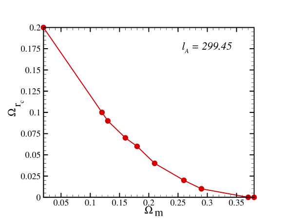
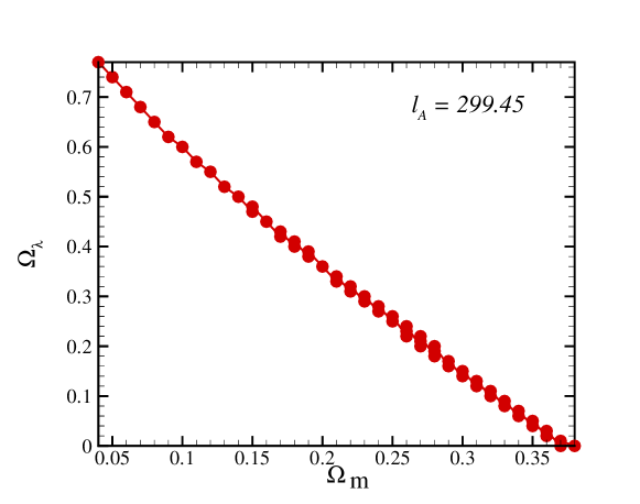
Figure 7: Constant acoustic angular scale in the joint space of $\Omega_{m}$ and $\Omega_{r_{c}}$ (upper panel). Lower panel shows dependence of acoustic angular scale on the $\Omega_{m}$ and cosmological constant.

Using $\chi^{2}_{\rm SNIa}+\chi_{l_{1}}^{2}$ analysis, we find the best fit values as: $\Omega_{m}=0.15^{+0.03}_{-0.03}$, $\Omega_{r_{c}}=0.08_{-0.02}^{+0.02}$ imply $\Omega_{K}=0.42^{+0.10}_{-0.10}$ with $\chi^{2}_{min}/N_{d.o.f}=0.96$ for New catalog of Gold sample. For SNLS SNIa combined with the position of first peak we find: $\Omega_{m}=0.11^{+0.01}_{-0.01}$, $\Omega_{r_{c}}=0.11_{-0.01}^{+0.01}$ imply $\Omega_{K}=0.36^{+0.05}_{-0.05}$ with $\chi^{2}_{min}/N_{d.o.f}=0.85$ at $1\sigma$ level of confidence. Table 3 gives the best values of parameters using the location of first and third peaks of CMB power spectrum and other observational tests. We see that $\Omega_{m}$ and $\Omega_{r_{c}}$ are very sensitive to the peaks position of power spectrum of temperature fluctuations at the last scattering surface. Since the phase transitions of peak position are weakly model dependent we also apply the shift parameter of CMB to extract best values for model parameters. According to the $\chi_{\rm SNIa}^{2}+\chi_{\rm CMB}^{2}$ statistic we get: $\Omega_{m}=0.23^{+0.04}_{-0.03}$, $\Omega_{r_{c}}=0.14_{-0.01}^{+0.01}$ imply $\Omega_{K}=0.03^{+0.08}_{-0.06}$ with $\chi^{2}_{min}/N_{d.o.f}=0.93$ for new catalog of Gold sample. For SNLS SNIa combined with the position of first peak we find: $\Omega_{m}=0.17^{+0.02}_{-0.01}$, $\Omega_{r_{c}}=0.16_{-0.01}^{+0.01}$ imply $\Omega_{K}=0.05^{+0.05}_{-0.04}$ with $\chi^{2}_{min}/N_{d.o.f}=0.84$ at $1\sigma$ level of confidence. The corresponding age of the universe are $15.23_{-0.43}^{+0.50}$ and $14.48_{-0.19}^{+0.32}$, respectively. These values are slightly different than that of reported in the previous analysis zong ; maartens1 .

Table 2: The best values for the parameters of DGP self accelerating model with the corresponding age for the universe from fitting with SNIa from new Gold sample and SNLS data, SNIa+CMB+gas, SNIa+CMB+gas+SDSS and SNIa+CMB+gas+SDSS+LSS experiments at one and two $\sigma$ confidence level.

Observation	$\Omega_{m}$	$\Omega_{r_{c}}$	$\Omega_{K}$	Age (Gyr)
	$0.36^{+0.07}_{-0.06}$	$0.23^{+0.04}_{-0.04}$	$-0.56^{+0.20}_{-0.20}$
SNIa(new Gold)				$13.78^{+0.68}_{-0.59}$
	$0.36^{+0.13}_{-0.14}$	$0.23^{+0.09}_{-0.10}$	$-0.56^{+0.43}_{-0.48}$
SNIa(new Gold)	$0.23^{+0.04}_{-0.03}$	$0.14^{+0.02}_{-0.02}$	$0.04^{+0.11}_{-0.10}$
+CMB+gas				$15.23^{+0.64}_{-0.45}$
	$0.23^{+0.08}_{-0.06}$	$0.14^{+0.03}_{-0.03}$	$0.04^{+0.18}_{-0.16}$
SNIa(new Gold)	$0.30^{+0.01}_{-0.05}$	$0.12^{+0.02}_{-0.01}$	$0.01^{+0.09}_{-0.09}$
+CMB+SDSS				$14.52^{+0.15}_{-0.48}$
+gas	$0.30^{+0.04}_{-0.06}$	$0.12^{+0.03}_{-0.03}$	$0.01^{+0.15}_{-0.16}$
SNIa(new Gold)	$0.28^{+0.03}_{-0.02}$	$0.13^{+0.01}_{-0.01}$	$-0.002^{+0.064}_{-0.053}$
+CMB+SDSS				$14.55^{+0.32}_{-0.22}$
+LSS+gas	$0.28^{+0.05}_{-0.04}$	$0.13^{+0.02}_{-0.03}$	$-0.002^{+0.117}_{-0.144}$
	$0.13^{+0.06}_{-0.06}$	$0.14^{+0.03}_{-0.03}$	$0.20^{+0.16}_{-0.16}$
SNIa (SNLS)				$14.96^{+1.03}_{-1.43}$
	$0.13^{+0.13}_{-0.12}$	$0.14^{+0.06}_{-0.07}$	$0.20^{+0.33}_{-0.35}$
SNIa(SNLS)	$0.17^{+0.01}_{-0.01}$	$0.16^{+0.01}_{-0.01}$	$0.05^{+0.05}_{-0.05}$
+CMB+gas				$14.48^{+0.19}_{-0.19}$
	$0.17^{+0.03}_{-0.04}$	$0.16^{+0.02}_{-0.02}$	$0.05^{+0.10}_{-0.11}$
SNIa(SNLS)	$0.22^{+0.01}_{-0.01}$	$0.15^{+0.01}_{-0.01}$	$0.01^{+0.04}_{-0.04}$
+CMB+SDSS				$13.88^{+0.15}_{-0.15}$
+gas	$0.22^{+0.03}_{-0.03}$	$0.15^{+0.02}_{-0.02}$	$0.01^{+0.10}_{-0.10}$
SNIa(SNLS)	$0.21^{+0.01}_{-0.01}$	$0.16^{+0.01}_{-0.01}$	$0.01^{+0.04}_{-0.04}$
+CMB+SDSS				$13.88^{+0.15}_{-0.15}$
+LSS+gas	$0.21^{+0.03}_{-0.03}$	$0.16^{+0.02}_{-0.02}$	$0.01^{+0.10}_{-0.10}$

The recently detected size of baryonic peak in the SDSS is the third observational data for our analysis. The correlation function of 46,748 Luminous Red Galaxies (LRG) from the SDSS shows a well detected baryonic peak around $100h^{-1}$ Mpc. This peak was identified with the expanding spherical wave of baryonic perturbations originating from acoustic oscillations at recombination. This peak has an excellent match to the predicted shape and the location of the imprint of the recombination-epoch acoustic oscillation on the low-redshift clustering matter eisenstein05 . Recently Linder has shown in detail some systematic uncertainties for baryon acoustic oscillation linder . Nonlinear mode coupling which is related to this fact that the baryon acoustic oscillation is mostly contributed by linear scale, but the influence of non-linear collapsing has quite broad kernel. In other words, one might say that baryon acoustic oscillation are $90-99\%$ linear in comparison to the CMB which is $99.99\%$ linear, so this difference may affect on various models in different way. Careful works to constrain on the free parameters of underlying model needs to be carried out to determine the effect of nonlinear mode coupling in the results of constraint by SDSS observation. Nevertheless, roughly speaking regards the acceptance intervals for free parameter cover the real intervals determined by assuming nonlinearity mode for SDSS observation Amarzguioui .

A dimensionless and independent of $H_{0}$ version of SDSS observational parameter is:

$${\cal A} = D_{V}(z_{\rm sdss})\frac{\sqrt{\Omega_{m}H_{0}^{2}}}{z_{\rm sdss}}$$ (47)

$$= \sqrt{\Omega_{m}}\left[\frac{H_{0}D_{L}^{2}(z_{\rm sdss};\Omega_{m},\Omega_{r_{c}})}{H(z_{\rm sdss};\Omega_{m},\Omega_{r_{c}})z_{\rm sdss}^{2}(1+z_{\rm sdss})^{2}}\right]^{1/3}.$$

where $D_{V}(z_{\rm sdss})$ is characteristic distance scale of the survey with mean redshift $z_{\rm sdss}$ eisenstein05 ; blak03 ; ness06 . We use the robust constraint on the DGP model using the value of ${\cal A}=0.469\pm 0.017$ from the Luminous Red Galaxy (LRG) observation at $z_{\rm sdss}=0.35$ eisenstein05 . This observation permits the addition of one more term in the $\chi^{2}$ of equations (34) and (46) to be minimized with respect to $H(z)$ model parameters. This term is:

$$\chi_{\rm SDSS}^{2}=\frac{\left[{\cal A}_{\rm obs}-{\cal A}_{\rm th}\right]^{2}}{\sigma_{\rm sdss}^{2}}$$ (48)

The baryon gas mass fraction for a range of redshifts is another observational test, can also be used to constrain cosmological models $H(z)$. The basic assumption corresponding to this method is related to the baryon gas mass fraction in clusters allen04 ; allen02 ; arn05 as:

$$S_{\rm gas}=\frac{M_{{\rm b}-{\rm gas}}}{M_{\rm tot}}$$ (49)

this quantity is constant, related to the global fraction of the universe $\Omega_{b}/\Omega_{m}$. $S_{\rm gas}$ can be written as:

$$S_{\rm gas}=\frac{1}{(1+\beta)}\frac{M_{{\rm b}}}{M_{\rm tot}}=\frac{b}{(1+\beta)}\frac{\Omega_{b}}{\Omega_{m}}$$ (50)

where $b$ is a bias factor suggesting that the baryon fraction in clusters is slightly lower than for the universe as a whole. Also $1+\beta$ is a factor taking into account the fact that the total baryonic mass in clusters consists of both X-ray gas and optically luminous baryonic mass (stars), the later being proportional to the former with proportionality constant $\beta\simeq 0.19\sqrt{h}$ allen04 . Dimensionless parameter for this observation is given by ness06 :

$${\cal{S}}_{\rm gas}(z;\Omega_{m},\Omega_{r_{c}}) = \frac{b}{1+\beta}\frac{\Omega_{b}}{\Omega_{m}}\left(\frac{D_{A}^{\rm flat}(z)}{D_{A}(z;\Omega_{m},\Omega_{r_{c}})}\right)^{\frac{3}{2}}$$ (51)

$$= \xi\left(\frac{D_{L}^{\rm flat}(z)}{D_{L}(z;\Omega_{m},\Omega_{r_{c}})}\right)^{\frac{3}{2}}$$

where $D_{A}^{\rm flat}$ is the angular diameter distance corresponding to flat pure CDM ($\Omega_{m}=1$). Least square quantity in the likelihood analysis for this observation is:

$$\chi^{2}(\xi,\Omega_{m},\Omega_{r_{c}}) = \sum_{i}\frac{[{\cal S}_{\rm gas}^{\rm obs}(z_{i})-{\cal S}_{\rm gas}^{\rm th}(z_{i};\Omega_{m},\Omega_{r_{c}},\xi)]^{2}}{\sigma_{i}^{2}},$$

Marginalizing over the nuisance parameter, $\xi$ gives:

$$\chi^{2}_{\rm gas}(\Omega_{m},\Omega_{r_{c}})=K-\frac{W^{2}}{Y}$$ (53)

where

$$K=\sum_{i}\frac{{\cal S}_{\rm gas}^{\rm obs}(z_{i})^{2}}{\sigma_{i}^{2}}$$ (54)

$$W=\sum_{i}\frac{{\cal S}_{\rm gas}^{\rm obs}(z_{i})\cdot{\cal S}_{\rm gas}^{\rm th}(z_{i};\Omega_{m},\Omega_{r_{c}},\xi=1)}{\sigma_{i}^{2}}$$ (55)

and

$$Y=\sum_{i}\frac{{\cal S}_{\rm gas}^{\rm th}(z_{i};\Omega_{m},\Omega_{r_{c}},\xi=1)^{2}}{\sigma_{i}^{2}}$$ (56)

We use the $26$ cluster data for ${\cal{S}}_{\rm gas}^{\rm obs}(z)$ reported in Ref. allen04 to examine DGP modified gravity model. According to equations (34), (41), (42), (46), (48) and (53) we can constrain free parameters of the model using observational data set related to background evolution.

In what follows we perform a combined analysis of SNIa, CMB, gas cluster and SDSS to constrain the parameters of the DGP model by minimizing the combined $\chi^{2}=\chi^{2}_{\rm{SNIa}}+\chi^{2}_{{\rm CMB}}+\chi^{2}_{\rm gas}+\chi^{2}_{{\rm SDSS}}$. The best values of the model parameters from the fitting with the corresponding error bars from the likelihood function marginalizing over the Hubble parameter in the multidimensional parameter space are: $\Omega_{m}=0.30_{-0.05}^{+0.01}$, $\Omega_{r_{c}}=0.12_{-0.01}^{+0.02}$ and $\Omega_{K}=0.01^{+0.09}_{-0.09}$ at $1\sigma$ confidence level with $\chi^{2}_{min}/N_{d.o.f}=0.94$. The Hubble parameter corresponding to the minimum value of $\chi^{2}$ is $h=0.61$. Here we obtain an age of $14.52_{-0.48}^{+0.15}$ Gyr for the universe. Using the SNLS data, the best fit values of model parameters are: $\Omega_{m}=0.22_{-0.01}^{+0.01}$, $\Omega_{r_{c}}=0.15_{-0.01}^{+0.01}$ and $\Omega_{K}=0.01^{+0.04}_{-0.04}$ at $1\sigma$ confidence level with $\chi^{2}_{min}/N_{d.o.f}=0.85$. Table 2 indicates the best fit values for the cosmological parameters with one and two $\sigma$ level of confidence.

Using the peaks position we find different values for the present matter density and $\Omega_{r_{c}}$. Table 3 illustrates the best fit values and corresponding derived age of universe. According to the values reported in Tables 2 and 3, we infer that the value of $\Omega_{r_{c}}$ is very sensitive to the observational results from CMB. As usual we take the values confined using shift parameter of CMB instead of one given by absolute values from peaks position as a reliable results.

Table 3: The best values for the parameters of DGP self accelerating model with the corresponding age for the universe from fitting with SNIa from new Gold sample and SNLS data, SNIa+first peak and SNIa+first peak+SDSS+LSS also for third peak experiments at one and two $\sigma$ confidence level.

Observation	$\Omega_{m}$	$\Omega_{r_{c}}$	$\Omega_{K}$	Age (Gyr)
SNIa(new Gold)	$0.15^{+0.03}_{-0.03}$	$0.08^{+0.02}_{-0.02}$	$0.42^{+0.10}_{-0.10}$
+First Peak				$15.86^{+0.48}_{-0.54}$
	$0.15^{+0.06}_{-0.05}$	$0.08^{+0.03}_{-0.03}$	$0.42^{+0.16}_{-0.16}$
SNIa(new Gold)	$0.30^{+0.01}_{-0.01}$	$0.01^{+0.02}_{-0.04}$	$0.57^{+0.08}_{-0.08}$
+First Peak+				$13.77^{+0.09}_{-0.09}$
SDSS+LSS	$0.30^{+0.02}_{-0.04}$	$0.01^{+0.02}_{-0.01}$	$0.57^{+0.09}_{-0.09}$
SNIa(new Gold)	$0.13^{+0.04}_{-0.01}$	$0.09^{+0.01}_{-0.02}$	$0.41^{+0.08}_{-0.09}$
+Third Peak				$16.30^{+0.66}_{-0.28}$
	$0.13^{+0.08}_{-0.02}$	$0.09^{+0.02}_{-0.05}$	$0.41^{+0.16}_{-0.21}$
SNIa(new Gold)	$0.29^{+0.01}_{-0.02}$	$0.01^{+0.01}_{-0.01}$	$0.58^{+0.08}_{-0.08}$
+Third Peak+				$13.85^{+0.09}_{-0.09}$
SDSS+LSS	$0.29^{+0.02}_{-0.07}$	$0.01^{+0.02}_{-0.01}$	$0.58^{+0.15}_{-0.11}$
SNIa(SNLS)	$0.11^{+0.01}_{-0.01}$	$0.11^{+0.01}_{-0.01}$	$0.36^{+0.05}_{-0.05}$
+First Peak				$14.99^{+0.22}_{-0.23}$
	$0.11^{+0.02}_{-0.02}$	$0.11^{+0.02}_{-0.02}$	$0.36^{+0.09}_{-0.09}$
SNIa(SNLS)	$0.15^{+0.01}_{-0.01}$	$0.08^{+0.01}_{-0.01}$	$0.42^{+0.05}_{-0.05}$
+First Peak+				$14.25^{+0.16}_{-0.16}$
SDSS+LSS	$0.15^{+0.02}_{-0.03}$	$0.08^{+0.02}_{-0.02}$	$0.42^{+0.09}_{-0.09}$
SNIa(SNLS)	$0.08^{+0.01}_{-0.01}$	$0.13^{+0.01}_{-0.01}$	$0.33^{+0.04}_{-0.04}$
+Third Peak				$15.91^{+0.29}_{-0.31}$
	$0.08^{+0.02}_{-0.02}$	$0.13^{+0.02}_{-0.02}$	$0.33^{+0.09}_{-0.09}$
SNIa(SNLS)	$0.16^{+0.03}_{-0.03}$	$0.07^{+0.02}_{-0.01}$	$0.45^{+0.10}_{-0.09}$
+Third Peak+				$14.04^{+0.40}_{-0.43}$
SDSS+LSS	$0.16^{+0.04}_{-0.04}$	$0.07^{+0.03}_{-0.02}$	$0.45^{+0.14}_{-0.11}$

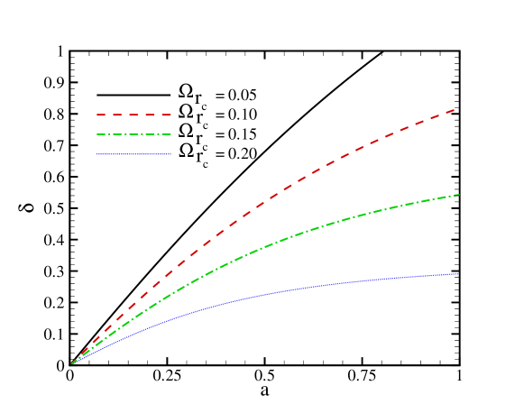
Figure 8: Evolution of density contrast as a function of scale factor for different values of $\Omega_{r_{c}}$ in a flat universe.

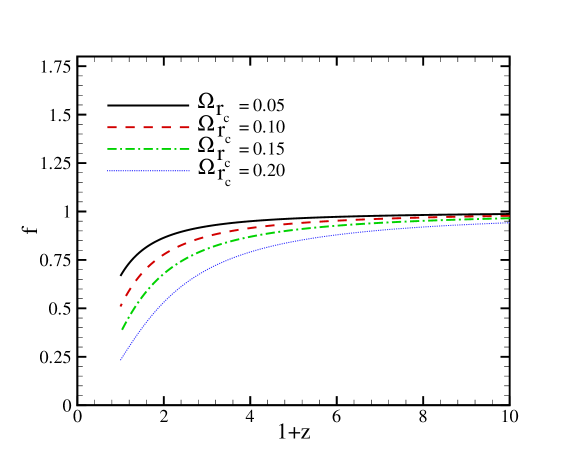
Figure 9: Growth index versus redshift for different values of $\Omega_{r_{c}}$. Here we imagined flat universe.

4 Constraints by Large Scale structure

So far we have only considered observational results related to the background evolution. In this section using the linear approximation of structure formation we obtain the growth index of structures and compare it with the result of observations by the $2$-degree Field Galaxy Redshift Survey ($2$dFGRS).

Koyama and Maartens maartens2 have recently shown the evolution of density perturbations requires an analysis of the 5-dimensional gravitational field. In this model Poisson equation is modified and shows the suppression of growth due to gravity leakage. The continuity and modified Poisson equations for the density contrast $\delta=\delta\rho/\bar{\rho}$ in the cosmic fluid provide the evolution of density contrast in the linear approximation (i.e. $\delta\ll 1$)maartens2 ; P93 ; B04 as:

$$\ddot{\delta}+2\frac{\dot{a}}{a}\dot{\delta}-\left[{v_{s}}^{2}\nabla^{2}+4\pi G\left(1+\frac{1}{3\alpha}\right)\rho\right]\delta=0,$$ (57)

where

$$\alpha=1-2r_{c}H\left(1+\frac{\dot{H}}{3H^{2}}\right)$$ (58)

the dot denotes the derivative with respect to time. Thus the growth rate receives an additional modification from the time variation of Newton s constant through $\alpha$.

The effect of dark energy in the evolution of the structures in this equation enters through its influence on the expansion rate. The validity of this linear Newtonian approach is restricted to perturbations on the sub-horizon scales but large enough where structure formation is still in the linear regime maartens2 ; P93 ; B04 . For the perturbations larger than the Jeans length, $\lambda_{J}=\pi^{1/2}v_{s}/\sqrt{G\left(1+\frac{1}{3\alpha}\right)\rho}$, equation (57) for cold dark matter (CDM) reduces to:

$$\ddot{\delta}+2\frac{\dot{a}}{a}\dot{\delta}-4\pi G\left(1+\frac{1}{3\alpha}\right)\rho\delta=0$$ (59)

The equation for the evolution of density contrast can be rewritten in terms of the scale factor as:

$$\frac{d^{2}\delta}{da^{2}}+\frac{d\delta}{da}\left[\frac{\ddot{a}}{\dot{a}^{2}}+\frac{2H}{\dot{a}}\right]-\frac{3H_{0}^{2}}{2\dot{a}^{2}a^{3}}\left(1+\frac{1}{3\alpha}\right)\Omega_{m}\delta=0.$$ (60)

Numerical solution of equation (60) in the FRW universe in the background of DGP model is shown in Figure 8. In the CDM model, the density contrast $\delta$ grows linearly with the scale factor, while we have a deviation from the linearity as soon as universe enters to acceleration era. Increasing $\Omega_{r_{c}}$ leads a decreasing in the evolution of density contrast which is in agreement to the finding about the behavior acceleration parameter versus $\Omega_{r_{c}}$ (see Figure 1).

In the linear perturbation theory, the peculiar velocity field $\bf{v}$ is determined by the density contrast P93 ; P80 as:

$${\bf v}({\bf x})=H_{0}\frac{f}{4\pi}\int\delta({\bf y})\frac{{\bf x}-{\bf y}}{\left|{\bf x}-{\bf y}\right|^{3}}d^{3}{\bf y},$$ (61)

where the growth index $f$ is defined by:

$$f=\frac{d\ln\delta}{d\ln a},$$ (62)

and it is proportional to the ratio of the second term of equation (59) (friction) to the third (Poisson) term.

We use the evolution of the density contrast $\delta$ to compute the growth index of structure $f$, which is an important quantity for the interpretation of peculiar velocities of galaxies, as discussed in P80 ; rah02 for the Newtonian and the relativistic regime of structure formation. Replacing the density contrast with the growth index in equation (60) results in the evolution of growth index as:

$$\frac{df}{d\ln a}=\frac{3H_{0}^{2}}{2\dot{a}^{2}a}\left(1+\frac{1}{3\alpha}\right)\Omega_{m}-f^{2}-f\left[1+\frac{\ddot{a}}{aH^{2}}\right]$$ (63)

Figure 9 shows the numerical solution of equation (63) in terms of redshift. An analytic formula for the present growth index in the flat $\Lambda$CDM model has been given in ref. f as $f(z=0.0,\Omega_{m})\simeq\Omega_{m}^{0.6}$, here we extend this formula for the universe governed by DGP modified gravity. The simplest form for fitting formula in the wide range of $\Omega_{m}$ and $\Omega_{r_{c}}$ is

$$f(z=0.0;\Omega_{m},\Omega_{r_{c}}) \simeq \Omega_{m}^{0.6}+\left(0.0159+0.0603\Omega_{m}\right)\times$$ (64)

$$\exp\biggl{(}\left[1.0694-0.3867\ln\Omega_{m}\right]^{2}\Omega_{r_{c}}\biggr{)}$$

$$-0.0542\Omega_{m}-0.0100$$

Figure 10 shows growth index, $f(z=0.0;\Omega_{m}=0.30)$, as a function of $\Omega_{r_{c}}$ derived from numerical solution of equation (63) and illustrated by fitting formula (equation (64)).

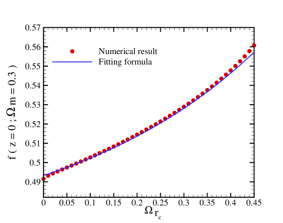
Figure 10: Growth index versus $\Omega_{r_{c}}$ for $z=0.0$ and $\Omega_{m}=0.30$. Solid line is given by fitting formula and symbol is derived by numerical solution of equation (63).

To use observational results implied to linear structure formation we rely to the observation of $220,000$ galaxies with the $2$dFGRS experiment provides the numerical value of growth index eisenstein05 . By measurements of two-point correlation function, the $2$dFGRS team reported the redshift distortion parameter of $\varepsilon=f/\kappa=0.49\pm 0.09$ at $z=0.15$, where $\kappa$ is the bias parameter describing the difference in the distribution of galaxies and their masses. Verde et al. (2003) used the bispectrum of $2$dFGRS galaxies ver01 ; la02 and obtained $\kappa_{verde}=1.04\pm 0.11$ which gave $f=0.51\pm 0.10$. Now we fit the growth index at the present time derived from the equation (63) with the observational value. This fitting gives a less constraint to the parameters of the model, so in order to have a better confinement of the parameters, we combine this fitting with those of SNIa$+$CMB$+$SDSS which have been discussed in the previous section. We perform the least square fitting by minimizing $\chi^{2}=\chi_{\rm{SNIa}}^{2}+\chi_{\rm{CMB}}^{2}+\chi_{\rm gas}^{2}+\chi_{\rm{SDSS}}^{2}+\chi_{\rm{LSS}}^{2}$, where

$$\chi^{2}_{\rm{LSS}}=\frac{[f_{obs}(z=0.15)-f_{th}(z=0.15;\Omega_{m},\Omega_{r_{c}})]^{2}}{\sigma_{f_{obs}}^{2}}$$ (65)

The best fit values with the corresponding error bars for the model parameters by using new Gold sample data are: $\Omega_{m}=0.28^{+0.03}_{-0.02}$, $\Omega_{r_{c}}=0.13_{-0.01}^{+0.01}$ and $\Omega_{K}=-0.002_{-0.053}^{+0.064}$ at $1\sigma$ confidence level with $\chi^{2}_{min}/N_{d.o.f}=0.93$. Using the SNLS supernova data, the best fit values for model parameters are: $\Omega_{m}=0.21^{+0.01}_{-0.01}$, $\Omega_{r_{c}}=0.16_{-0.01}^{+0.01}$ and $\Omega_{K}=0.01_{-0.04}^{+0.04}$ at $1\sigma$ confidence level with $\chi^{2}_{min}/N_{d.o.f}=0.84$. The error bars have been obtained through the likelihood functions $(\mathcal{L}$$\propto e^{-\chi^{2}/2})$ marginalized over the nuisance parameter $h$ press94 . The best values reported in the Ref. maartens1 using SNIa+CMB+SDSS are: $\Omega_{m}=0.270$, $\Omega_{r_{c}}=0.125$ for Gold sample SNIa and for SNLS SNIa are: $\Omega_{m}=0.255$, $\Omega_{r_{c}}=0.130$, while in Ref. zong using SNIa+SDSS, $\Omega_{m}=0.270_{+0.018}^{-0.017}$, $\Omega_{r_{c}}=0.216_{-0.013}^{+0.012}$. We concluded that observational results from large scale structure given by $2$dfGRS in addition to including baryon gas mass fraction results, put weak constraints on the DGP model free parameters.

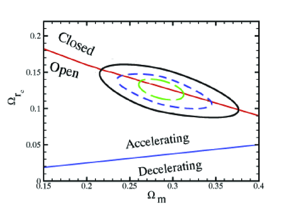
Figure 15: Joint confidence intervals of $\Omega_{m}$ and $\Omega_{r_{c}}$, fitted with SNIa new Gold sample$+$CMB$+$gas$+$SDSS$+$LSS. Solid line, dashed line and long dashed line correspond to $3\sigma$, $2\sigma$ and $1\sigma$ level of confidence, respectively.

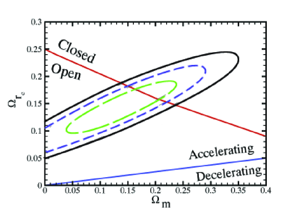
Figure 16: Joint confidence intervals of $\Omega_{m}$ and $\Omega_{r_{c}}$, fitted with SNIa SNLS. Solid line, dashed line and long dashed line correspond to $3\sigma$, $2\sigma$ and $1\sigma$ level of confidence, respectively.

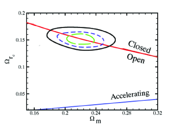
Figure 17: Joint confidence intervals of $\Omega_{m}$ and $\Omega_{r_{c}}$, fitted with SNIa SNLS$+$CMB$+$gas$+$SDSS$+$LSS. Solid line, dashed line and long dashed line correspond to $3\sigma$, $2\sigma$ and $1\sigma$ level of confidence, respectively.

The likelihood functions for the three cases of (i) fitting model with Supernova data, (ii) combined analysis with the three experiments of SNIa$+$CMB$+$gas and (iii) combining all five experiments of SNIa$+$CMB$+$gas$+$SDSS$+$LSS are shown in Figures 12 and 13. The joint confidence contours in the $(\Omega_{m},\Omega_{r_{c}})$ plane are also shown in Figures 14 and 15 for Gold sample and combined observational results, respectively. Figures 16 and 17 show the joint confidence interval for SNLS data and SNIa$+$CMB$+$gas$+$SDSS$+$LSS experiments.

5 Age of Universe

The ”age crisis” is one the main reasons of the acceleration phase of the universe. The problem is that the universe’s age in the Cold Dark Matter (CDM) universe is less than the age of old stars in it. Studies on the old stars carretta00 suggest an age of $13^{+4}_{-2}$ Gyr for the universe. Richer et. al. richer02 and Hasen et. al. hansen02 also proposed an age of $12.7\pm 0.7$ Gyr, using the white dwarf cooling sequence method (for full review of the cosmic age see spe03 ). The age of universe integrated from the big bang up to now is given by:

$$t_{0}(\Omega_{m},\Omega_{r_{c}}) = \int_{0}^{t_{0}}\,dt$$ (66)

$$= \int_{0}^{\infty}{dz^{\prime}\over(1+z^{\prime})H(z^{\prime})}$$

Figure 11 shows the dependence of $H_{0}t_{0}$ (Hubble parameter times the age of universe) on $\Omega_{r_{c}}$ for a flat universe. Obviously increasing $\Omega_{r_{c}}$ results in a longer age for the universe. As shown in the lower panel of Figure 11, $\Omega_{r_{c}}$ behaves as the same as dark energy, $\Omega_{\Lambda}$, in the flat $\Lambda$CDM model.

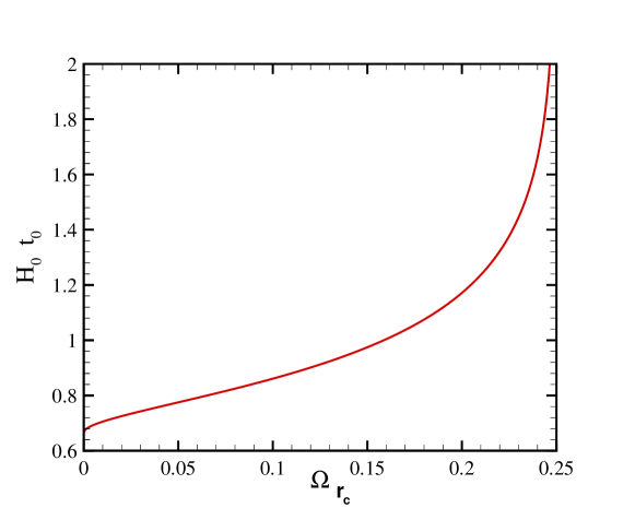
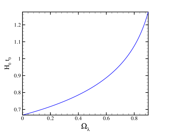
Figure 11: $H_{0}t_{0}$ (age of universe times the Hubble constant at the present time) as a function of $\Omega_{r_{c}}$ in a flat universe. Increasing $\Omega_{r_{c}}$ gives a longer age for the universe. Lower panel shows the same function versus $\Omega_{\lambda}$ in the flat $\Lambda$CDM model and $w=-1.0$.

Finally we do the consistency test, comparing the age of universe derived from this model with the age of old stars and Old High Redshift Galaxies (OHRG) in various redshifts. Table 2 shows that the age of universe from the combined analysis of SNIa$+$CMB$+$gas$+$SDSS$+$LSS is $14.55_{-0.22}^{+0.32}$ Gyr and $13.88_{-0.15}^{+0.15}$ for new Gold sample and SNLS data, respectively. These values are in agreement with the age of old stars carretta00 . Here we take three OHRG for comparison with the DGP model, namely the LBDS $53$W$091$, a $3.5$-Gyr old radio galaxy at $z=1.55$ dunlop96 , the LBDS $53$W$069$ a $4.0$-Gyr old radio galaxy at $z=1.43$ dunlop99 and a quasar, APM $08279+5255$ at $z=3.91$ with an age of $t=2.1_{-0.1}^{+0.9}$Gyr hasinger02 . The latter has once again led to the ”age crisis”. An interesting point about this quasar is that it cannot be accommodated in the $\Lambda$CDM model jan06 . To quantify the age-consistency test we introduce the expression $\tau$ as:

$$\tau=\frac{t(z;\Omega_{m},\Omega_{r_{c}})}{t_{obs}}=\frac{t(z;\Omega_{m},\Omega_{r_{c}})H_{0}}{t_{obs}H_{0}},$$ (67)

where $t(z)$ is the age of universe, obtained from the equation (66) and $t_{obs}$ is an estimation for the age of old cosmological object. In order to have a compatible age for the universe we should have $\tau>1$. Table 4 shows the value of $\tau$ for three mentioned OHRG. We see that the parameters of DGP model from the combined observations don’t provide a compatible age for the universe, compared to the age of old objects, while the SNLS data result in a longer age for the universe. Once again for the DGP model, APM $08279+5255$ at $z=3.91$ has a longer age than the universe but gives better results than most Quintessence and braneworld models sa1 ; sa2 ; sa3 ; sa4 .

Table 4: The value of $\tau$ for three high redshift objects, using the parameters of the model derived from fitting with the observations.

Observation	LBDS	LBDS	APM
	$53$W$069$	$53$W$091$	$08279+5255$
	$z=1.43$	$z=1.55$	$z=3.91$
SNIa (new Gold)	$1.37^{+0.12}_{-0.12}$	$1.12^{+0.10}_{-0.10}$	$0.79^{+0.07}_{-0.07}$
SNIa(new Gold)+CMB	$1.35^{+0.03}_{-0.08}$	$1.11^{+0.03}_{-0.07}$	$0.83^{+0.02}_{-0.06}$
+SDSS+gas
SNIa(new Gold)+CMB	$1.37^{+0.05}_{-0.03}$	$1.12^{+0.04}_{-0.03}$	$0.84^{+0.03}_{-0.03}$
+SDSS+LSS+gas
SNIa (SNLS)	$1.53^{+0.17}_{-0.23}$	$1.26^{+0.14}_{-0.19}$	$1.00^{+0.13}_{-0.21}$
SNIa(SNLS)+CMB	$1.36^{+0.03}_{-0.03}$	$1.12^{+0.02}_{-0.02}$	$0.85^{+0.02}_{-0.02}$
+SDSS+gas
SNIa(SNLS)+CMB	$1.36^{+0.03}_{-0.03}$	$1.12^{+0.02}_{-0.02}$	$0.85^{+0.02}_{-0.02}$
+SDSS+LSS+gas

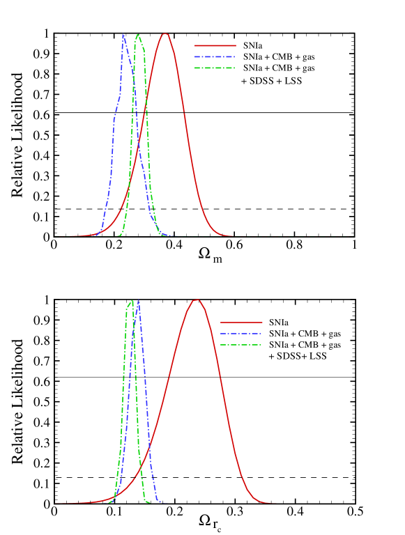
Figure 12: Marginalized likelihood functions of two parameters of DGP model ($\Omega_{m}$ and $\Omega_{r_{c}}$). The solid line corresponds to the likelihood function of fitting the model with SNIa data (new Gold sample), the dashdot line with the joint SNIa$+$CMB$+$gas data and dashed line corresponds to SNIa$+$CMB$+$gas$+$SDSS$+$LSS. The intersections of the curves with the horizontal solid and dashed lines give the bounds with $1\sigma$ and $2\sigma$ level of confidence respectively.

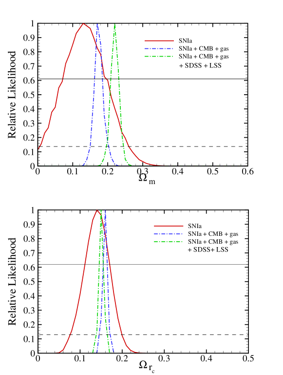
Figure 13: Marginalized likelihood functions of two parameters of DGP model ($\Omega_{m}$ and $\Omega_{r_{c}}$). The solid line corresponds to the likelihood function of fitting the model with SNIa data (SNLS), the dashdot line with the joint SNIa$+$CMB$+$gas data and dashed line corresponds to SNIa$+$CMB$+$gas$+$SDSS$+$LSS. The intersections of the curves with the horizontal solid and dashed lines give the bounds with $1\sigma$ and $2\sigma$ level of confidence respectively.

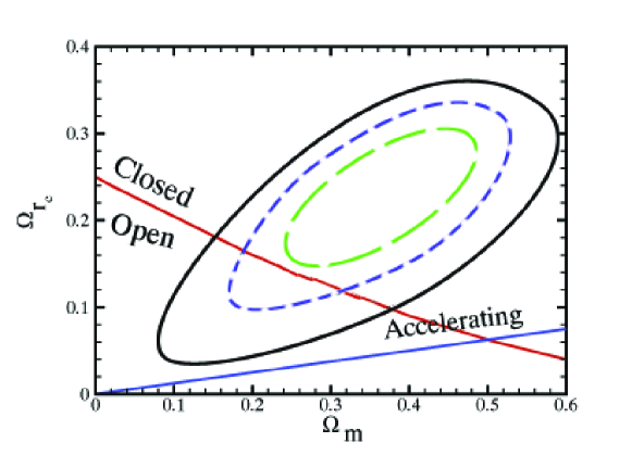
Figure 14: Joint confidence intervals of $\Omega_{m}$ and $\Omega_{r_{c}}$, fitted with SNIa new Gold sample. Solid line, dashed line and long dashed line correspond to $3\sigma$, $2\sigma$ and $1\sigma$ level of confidence, respectively.

6 Conclusion

We studied a self accelerating cosmological model, DGP modified gravity. The effect of this model on the age of universe, the radial comoving distance, the comoving volume element and the variation of the apparent size of objects with the redshift (Alcock-Paczynski test) have been studied. The evolution of density contrast, $\delta$, as a function of scale factor for various values of $\Omega_{r_{c}}$ shows that increasing $\Omega_{r_{c}}$ suppresses the growth of density contrast, which is in agreement with the behavior of acceleration parameter versus $\Omega_{r_{c}}$. We extrapolate the relation of the growth factor in terms of $\Omega_{i}$ to the present time and showed that the power-law term is the dominant term the DGP model. To constrain the parameters of model we fit our model with the new Gold sample and SNLS supernova data, CMB shift parameter, position of the first and third peaks of power spectrum of temperature fluctuations at the last scattering surface, the Cluster Baryon Gas Mass Fraction, location of baryonic acoustic oscillation peak observed by SDSS and large scale structure formation data by $2$dFGRS. The best parameters obtained from fitting with the new Gold sample data are: $h=0.62$, $\Omega_{m}=0.28^{+0.03}_{-0.02}$, $\Omega_{r_{c}}=0.13_{-0.01}^{+0.01}$ and $\Omega_{K}=-0.002_{-0.053}^{+0.064}$ at $1\sigma$ confidence level with $\chi^{2}_{min}/N_{d.o.f}=0.93$ and by using the SNLS data are: $\Omega_{m}=0.22^{+0.01}_{-0.01}$, $\Omega_{r_{c}}=0.15_{-0.01}^{+0.01}$ and $\Omega_{K}=0.01_{-0.04}^{+0.04}$ at $1\sigma$ confidence level with $\chi^{2}_{min}/N_{d.o.f}=0.84$. Comparing our results to that of previous results zong ; maartens1 showed that large scale structure observations from $2$dFGRS experiment had weak effect on confining the acceptance intervals for the free parameters. The observational constraint just by using SNIa+CMB indicated that our universe is spatially open but combining these result with SDSS+gas+LSS showed that our universe in the DGP model is very good agreement with the spatially flat universe. In comparison between $\Lambda$CDM and DGP in terms of $\chi^{2}_{\nu}$, Table 5 shows that these two models result almost same values.

Table 5: The value of $\chi^{2}_{\nu}$ for $\Lambda$CDM and DGP modified gravity models.

Observation	$\Lambda$CDM	DGP
SNIa (new Gold)	$0.92$	$0.91$
SNIa(new Gold)+CMB	$0.93$	$0.94$
+SDSS
SNIa(new Gold)+CMB	$0.93$	$0.93$
+SDSS+LSS
SNIa (SNLS)	$0.87$	$0.85$
SNIa(SNLS)+CMB	$0.86$	$0.85$
+SDSS
SNIa(SNLS)+CMB	$0.85$	$0.84$
+SDSS+LSS

We also performed the age test, comparing the age of old stars and old high redshift galaxies with the age derived from this model. From the best fit parameters of the model using new Gold sample and SNLS SNIa, we obtained an age of $14.55_{-0.22}^{+0.32}$ Gyr and $13.88_{-0.15}^{+0.15}$ Gyr, respectively, for the universe which is in agreement with the age of old stars. We also chose two high redshift radio galaxies at $z=1.55$ and $z=1.43$ with a quasar at $z=3.91$. The ages of the two first objects were consistent with the age of universe, i.e.,they were younger than the universe while the third one was not.

References

- (1) A. G. Riess et al., Astron. J. 116, 1009 (1998).
- (2) S. Perlmutter et al., Astrophys. J. 517, 565 (1999).
- (3) C. L. Bennett et al., Astrophys. J. Suppl. Ser. 148, 1 (2003).
- (4) H.V. Peiris et al., Astrophys. J. Suppl. Ser. 148, 213 (2003).
- (5) D. N. Spergel, L. Verde, H. V. Peiris et al., Astrophys. J. 148, 175 (2003).
- (6) S. Weinberg, Rev. Mod. Phys. 61, 1 (1989; S. M. Carroll, Living Rev. Relativity 4, 1 (2001); P. J. E. Peebles and B. Ratra, Rev. Mod. Phys. 75, 559 (2003); T. Padmanabhan, Phys. Rep. 380, 235 (2003).
- (7) C. Wetterich, Nucl. Phys. B302, 668 (1988); P. J. E. Peebles and B. Ratra, Astrophys. J. 325, L17 (1988); B. Ratra and P. J. E. Peebles, Phys. Rev. D 37, 3406 (1988); J. A. Frieman, C. T. Hill, A. Stebbins, and I. Waga, Phys. Rev. Lett. 75, 2077 (1995); M. S. Turner and M. White, Phys. Rev. D 56, R4439 (1997); R. R. Caldwell, R. Dave, and P. J. Steinhardt, Phys. Rev. Lett. 80, 1582 (1998); A. R. Liddle and R. J. Scherrer, Phys. Rev. D 59, 023509 (1999); I. Zlatev, L.Wang, and P. J. Steinhardt, Phys. Rev. Lett. 82, 896 (1999); P. J. Steinhardt, L. Wang, and I. Zlatev, Phys. Rev. D 59, 123504 (1999); D. F. Torres, Phys. Rev. D 66, 043522 (2002).
- (8) L. Amendola, Phys. Rev. D 62, 043511 (2000); L. Amendola and D. Tocchini-Valentini, Phys. Rev. D 64, 043509 (2001); 66, 043528 (2002); L. Amendola, Mon. Not. R. Astron. Soc. 342, 221 (2003); M. Pietroni, Phys. Rev. D 67, 103523 (2003); D. Comelli, M. Pietroni, and A. Riotto, Phys. Lett. B 571, 115 (2003); U. Franca and R. Rosenfeld, Phys. Rev. D 69, 063517 (2004); X. Zhang, astro-ph/0503072; Phys. Lett. B 611, 1 (2005).
- (9) P. J. E. Peebles, R. Ratra, Astrophys. J. 325, L17 (1988).
- (10) C. Armendariz-Picon, V. Mukhanov and P. J. Steinhardt, Phys. Rev. Lett. 85, 4438 (2000).
- (11) J. S. Bagla, H. K. Jassal and T. Padmanabhan, Phys. Rev. D 67, 063504 (2003).
- (12) R. R. Caldwell, Phys. Lett. B 545, 23 (2002).
- (13) R. R. Caldwell, M. Kamionkowski and N. N. Weinberg, Phys. Rev. Lett. 91, 071301 (2003).
- (14) A. Kamenshchik, U. Moschella and V. Pasquier, Phys. Lett. B 511, 265 (2001).
- (15) L. Wang, R. R. Caldwell, J. P. Ostriker and P. J. Steinhardt, Astrophys. J. 530, 17 (2000).
- (16) S. Perlmutter, M. S. Turner and M. White, Phys. Rev. Lett. 83, 670 (1999).
- (17) L. Page et al., Astrophys. Supp. J. 148, 233 (2003).
- (18) M. Doran, M. Lilley,J. Schwindt and C. Wetterich, Astrophys. J. 559, 501 (2001).
- (19) M. Doran, M. Lilley, Mon. Not.Roy. A. Soc. 330, 965 (2002).
- (20) R. R. Caldwell and M. Doran, Phys. Rev. D 69, 103517 (2004).
- (21) S. Arbabi-Bidgoli, M. S. Movahed and S. Rahvar, International Journal of Modern Physics D Vol. 15, No. 9 (2006) 1455 1472.
- (22) T. Clifton , J. D. Barrow , Phys. Rev. D 72, 103005 (2005); S. Nojiri and S. D. Odintsov, Phys. Rev. D 68, 123512 (2003); S. Nojiri and S. D. Odintsov, Phys. Lett. B 562, 147 (2003); C. Deffayet, G. Dvali and G. Gabadadze, Phys. Rev. D 65, 044023 (2002); K. Freese and M. Lewis, Phys. Lett. B 540, 1 (2002); M. Ahmed, S. Dodelson, P. B. Greene and R. Sorkin, Phys. Rev. D 69 103523(2004); N. Arkani-Hamed, S. Dimopoulos, G. Dvali and G. Gabadadze, hep-th/0209227; G. Dvali and M. S. Turner, Fermilab pub. 03040-A (2003).
- (23) A. Lue, Phys. Rev. D, 67, 064004 (2003). Lue, A. 2005, astro-ph/0510068 Lue, A., Scoccimarro, R. and Starkman, G. D. 2004, Phys. Rev. D, 69, 124015
- (24) A. Lue and G. D. Starkman, Phys. Rev. D, 67, 064002(2003)
- (25) A. Lue, R. Scoccimarro and G. D. Starkman, Phys. Rev. D, 69, 124015(2004).
- (26) Zong-Kuan Guo, Zong-Hong Zhu, J.S. Alcaniz and Yuan-Zhong Zhang, Astrophys.J. 646 (2006) 1.
- (27) C. Deffayet, S.J. Landau, J. Raux, M. Zaldarriaga, P. Astier, Phys. Rev. D 66 024019 (2002)
- (28) Avelino, P. P. and Martins, C. J. A. P. 2002, ApJ, 565, 661
- (29) Dabrowski, M. P., Godlowski, W. and Szydlowski, M. 2004, Gen. Rel. Grav. 36, 767
- (30) Alam, U. and Sahni, V. 2005, astro-ph/0511473
- (31) R. Maartens and E. Majerotto, Phys.Rev. D 74 (2006) 023004.
- (32) M. Sadegh Movahed, Shant Baghram and Sorab Rahvar, arXiv:0705.0889.
- (33) J. S. Alcaniz, Phys. Rev. D 65 123514 (2002)
- (34) J. S. Alcaniz, D. Jain and A. Dev, Phys. Rev. D 66, 067301 (2002)
- (35) D. Jain, A. Dev and J. S. Alcaniz, Phys. Rev. D 66, 083511 (2002)
- (36) Multamäki T., Gaztanaga E. and Manera M. 2003, MNRAS, 344, 761
- (37) Z.H. Zhu and J.S. Alcaniz, ApJ, 620, 7 (2005).
- (38) J. S. Alcaniz and Z. H. Zhu, Phys. Rev. D 71, 083513 (2005)
- (39) V. Barger, Y. Gao and D. Marfatia, arXiv:astro-ph/0611775
- (40) Malcolm Fairbairn and Ariel Goobar, Phys.Lett. B 642 (2006) 432-435.
- (41) Yong-Seon Song, Ignacy Sawicki and Wayne Hu, arXiv:astro-ph/0606286.
- (42) L. Sawichi and S. M. Carroll, arXiv:astro-ph/0510364.
- (43) Ahmad Sheykhi, Bin Wang and Rong-Gen Cai, arXiv:hep-th/0701198
- (44) K. Koyama and R. Maartens, JCAP 0601, 016 (2006), arXiv:astro-ph/0511634.
- (45) O. Lahav, P. B. Lilje, J. R. Primack and M. J. Rees, Mon. Not. R. Astron. Soc. 251, 128 (1991).
- (46) C. Alcock and B. Paczynski, Nature 281, 358 (1979).
- (47) A. G. Riess et al., Astrophys. J. 607, 665 (2004).
-
(48)
G. R. Dvali, G. Gabadadze and M. Porrati,
Phys. Lett. B 484, 112 (2000)
[arXiv:hep-th/0002190];
C. Deffayet, Phys. Lett. B 502, 199 (2001) [arXiv:hep-th/0010186]. - (49) A. Nicolis and R. Rattazzi, JHEP 0406, 059 (2004)
- (50) M. A. Luty, M. Porrati and R. Rattazzi, JHEP 0309, 029 (2003)
- (51) K. Koyama, Phys. Rev. D 72 , 123511 (2005)
- (52) C. de Rham, G. Dvali, S. Hofmann, J. Khoury, O. Pujolas, M. Redi and A. J. Tolley, Phys. Rev. Lett. 100, 251603 (2008)
- (53) The Gold dataset is available at http://braeburn.pha.jhu.edu/ ariess/R06.
- (54) S. W. Allen, R. W. Schmidt, H. Ebeling, A. C. Fabian and L. van Speybroeck, Mon. Not. Roy. Astron. Soc. 353, 457 (2004) [arXiv:astro-ph/0405340].
- (55) B. P. Schmidt et al., Astrophys. J. 507, 46 (1998).
- (56) J. L. Tonry et al., Astrophys. J. 594, 1 (2003).
- (57) B. J. Barris et al., Astrophys. J. 602, 571 (2004).
- (58) A. Melchiorri, L. Mersini, C.L. dman and M. Trodden, arXive:astro-ph/0211522.
- (59) W. L. Freedman rt al., Astrophys. J. Lett. 553, 47 (2001).
- (60) X. Zhang and F.Q. Wu, Phys. Rev. D 72, 043524 (2005)
- (61) S. Nesseris and L. Perivolaropoulos, Phys. Rev. D 70, 043531 (2004).
- (62) S. Nesseris and L. Perivolaropoulos, Phys. Rev. D 72, 123519 (2005).
- (63) C. L. Bennett, R. S, Hill and G. Hinshaw, Astrophys. J. Suppl. 148, 97 (2003).
- (64) Hu, W., Sugiyama, N., Silk, J., 1997, Nat, 386, 37 [astro-ph/9604166]
- (65) W. Hu and N. Sugiyama, Astrophys. J. 444, 489 (1995).
- (66) Hu, W., Fukugita, M., Zaldarriaga, M., Tegmark, M., 2000, astro-ph/0006436
- (67) Michael Doran and Matthew Lilley, arXiv:stro-ph/0104486.
- (68) J. R. Bond, G. Efstathiou, and M. Tegmark, Mon. Not. R. Astron. Soc. 291, L33 (1997); A. Melchiorri, L. Mersini, C. J. Odman, and M. Trodden, Phys. Rev. D 68, 043509 (2003); C. J. Odman, A. Melchiorri, M. P. Hobson, and A. N. Lasenby, Phys. Rev. D 67, 083511 (2003).
- (69) T. J. Pearson et al. (CBI Collaboration), Astrophys. J. 591, 556 (2003); C. L. Kuo et al. (ACBAR Collaboration), Astrophys. J. 600, 32 (2004).
- (70) D. J. Eisenstein et al., astro-ph/0501171.
- (71) E. V. Linder, arXiv:astro-ph/0507308; E. V. Linder, Phys. Rev. D 68, 083504 (2003).
- (72) W. Hu and N. Sugiyama, Astrophys. J. 471 (1996) 542; D. J. Eisenstein and W. Hu, Astrophys. J. 496 (1998) 605, M. Amarzguioui, O. Elgaroy, D.F. Mota, T. Multamaki, arXiv:astro-ph/0510519. D. J. Eisenstein and M. J.White, Phys. Rev. D 70 103523 (2004).
- (73) C. Blake and K. Glazebrook, Astrophys. J. 594, 665 (2003) [arXiv:astro-ph/0301632].
- (74) S. Nesseris and L. Perivolaropoulos, JCAP 0701 (2007) 018.
- (75) S. W. Allen, R. W. Schmidt and A. C. Fabian, Mon. Not. Roy. Astron. Soc. 334, L11 (2002) [arXiv:astro-ph/0205007].
- (76) M. Arnaud, arXiv:astro-ph/0508159.
- (77) Padmanabhan T., 1993, Structure Formation in the Universe. Cambridge Univ. Press
- (78) Brandenberger, R. H., 2004, in Breton N., Cervantes-Cota J. L., and Salgado, M., eds, Lecture Notes in Physics, , The early universe and observational cosmology, 646, p.127
- (79) Peebles, P. J. E., 1980, The Large Scale Structure of the Universe, Princeton University Press, Princeton, NJ
- (80) Mansouri, R., Rahvar, S, 2002, Int. J. Modern Phys. D, 11, 312
- (81) Verde L., Kamionkowski M., Mohr J. J., Benson A.J., 2001, MNRAS, 321, L7
- (82) Lahav O., Bridle S. L., Percival W. J., & the 2dFGRS Team, 2002, MNRAS, 333, 961
- (83) W. H. Press, S. A. Teukolsky, W. T. Vettering and B. P. Flannery, Numerical Recipes, Cambridge University Press, Cambridge, 1994.
- (84) E. Carretta et al., Astrophys. J. 533, 215 (2000); L. M. Krauss and B. Chaboyer, astro-ph/0111597; B. Chaboyer and L. M. Krauss, Astrophys. J. Lett. 567, L45 (2002).
- (85) H. B. Richer et al., Astrophys. J. 574, L151 (2002).
- (86) B. M. S. Hansen et al., Astrophys. J. 574, L155 (2002).
- (87) J. Dunlop et. al., Nature (London) 381, 581 (1996); H. Spinrard, Astrophys. J. 484, 581 (1997).
- (88) J. Dunlop, in The Most Distant Radio Galaxies, edited by H. J. A. Rottgering, P. Best, and M. D. Lehnert (Kluwer, Dordrecht, 1999), p. 71.
- (89) G. Hasinger, N. Schartel and S. Komossa, Astrophys. J. Lett. 573, L77 (2002); S. Komossa and G. Hasinger, astro-ph/0207321.
- (90) D. Jain., A. Dev., astro-ph/0509212 (accepted in Phys. Lett. B)
- (91) M. Sadegh Movahed and S. Rahvar, Phys.Rev. D 73 083518 (2006).
- (92) S. Rahvar and M. Sadegh Movahed, Phys. Rev. D 75 , 023512 (2007).
- (93) M. Sadegh Movahed and Sima Ghassemi, Phys. Rev. D 76, 084037 (2007).
- (94) M. Sadegh Movahed and Ahmad Sheykhi, Mon. Not. R. Astron. Soc. 388, 197- 210 (2008).