Bayesian Evidence for a Cosmological Constant using new High-Redshift Supernovae Data

Abstract

We carry out a Bayesian model selection analysis of different dark energy parametrizations using the recent luminosity distance data of high redshift supernovae from Riess et al. 2007 and from the new ESSENCE Supernova Survey. Including complementary cosmological datasets, we found substantial evidence ($\Delta\ln(E)\sim 1$) against a time-varying dark energy equation of state parameter, and against phantom dark energy models. We find a small preference for a standard cosmological constant over accelerating non-phantom models where $w$ is constant, but allowed to vary in the range $-1$ to $-0.33$.

1 Introduction

Over the last few years, observations of luminosity distances of Type Ia supernovae (SN-Ia) have established that the expansion of the Universe is accelerating(see e.g. Riess et al. (1998), Perlmutter et al. (1999), Riess et al. (2004), Astier et al. (2005), Bassett et al. (2004)). This result is now well confirmed and complemented by a large amount of independent observations such as, for example, the angular-diameter distance vs. redshift relation measured by Baryonic Acoustic Oscillations (BAO) experiments Eisenstein et al. (2005), the distortion of background images measured by weak lensing experiments Jarvis et al. (2005), the distance to the last scattering surface measured by Cosmic Microwave Background (CMB) experiments Spergel et al. (2006), galaxy clustering (Large Scale Structure, LSS)(see Efstathiou et al. (2002); Tegmark et al. (2006)) and, finally, the Integrated Sachs Wolfe effect, correlating LSS with CMB (see e.g Giannantonio et al. (2006)).

The recent analysis of Riess et al. (2007) has further confirmed in an impressive way these results, reporting the discovery of 21 new SN-Ia with the Hubble Space Telescope (HST). Together with a recalibration of previous HST-discovered SN-Ia, the full sample of $23$ SN-Ia at $z>1$ provides the highest-redshift sample known. This dataset has then been analyzed in combination with some of the aforementioned datasets providing new constraints on several dark energy properties (see e.g. Riess et al. (2007), Alam (2006), Gong and Wang (2006), Nesseris & Perivolaropoulos (2006), Barger et al. (2006)).

This increasing quality and number of experimental datasets is finally opening the possibility of falsifying cosmological theories and of discriminating between different theories. There have been many proposed explanations for this acceleration: the Einstein’s cosmological constant, a new fluid with negative pressure (constant or varying with time) (see e.g. Peebles & Ratra (2003)) or a modification of general relativity (see for example Dvali, Gabadadze, Porrati (2000)). However, to date, none of them is supported by a well-established fundamental theory. Moreover, since we know (almost) nothing about dark energy there is in principle no theoretical limit to the number of parameters that one might use to characterize it.

It is therefore timely not only to constrain the parameters of a specific dark energy model but also to establish reliable criteria to choose between different models.

As pointed out in Mukherjee, Parkinson, Liddle (2006) and Liddle et al. (2006a), there is an important difference between parameter fitting and model selection. In the first case we work in the context of a single theoretical model framework, and establish which choice of model parameters gives the best fit to the data. In a Bayesian interpretation, with flat priors the most likely model parameters will simply have the maximum likelihood and the lowest $\chi^{2}$ regardless of the degrees of freedom. More complicated models (with a larger number of free parameters) will normally produce better fits. However, in model selection, we wish to know which model is favoured, regardless of the values of the parameters. In choosing models, we should also look for simplicity, following somewhat a principle based on Occam’s Razor. Simplicity is of course in contrast with more parameters and we need then to weight the “need” for extra parameters. This can be accomplished by using the Bayesian Evidence, defined as the probability of the model given the data, and given by the average likelihood of a model over its prior parameter space:

$$E=P(\vec{D}|H)=\int\,d\vec{\theta}\,P(\vec{D}|\vec{\theta},H)P(\vec{\theta},H),$$ (1)

where $H$ is the model considered, $\vec{\theta}$ is the vector of the model parameters, $\vec{D}$ is the data, $P(\vec{\theta},H)$ is the prior and $P(\vec{D}|\vec{\theta},H)$ is the likelihood. For flat priors on the models, the probability of the model given the data is proportional to the Evidence.

In general, comparing two models, the term $P(\vec{D}|\vec{\theta},H)$ will be larger for the more complicated one (which has more parameters or the same number of parameters but with larger prior space), but, at the same time, it will have a lower $P(\vec{\theta},H)d\vec{\theta}$ compared to the simpler model. The first term indicates how well the model fits data, the second one indicates how simple is the model. Following the equation above we can assume that the best model will be the one with the greatest Evidence.

Jeffreys (1961) provides a useful guide to discriminate the difference between two models with $E_{1}$ and $E_{2}$:

$$1<\Delta\,\ln(E)<2.5\,\,(substantial)\\$$ (2)

$$2.5<\Delta\,\ln(E)<5\,\,(strong)\\$$ (3)

$$5<\Delta\,\ln(E)(decisive).\\$$ (4)

The Bayesian Evidence can therefore help us to choose between models because it establish a tension between the simplicity of a model and its power of fitting data.

In this paper we aim exactly to make use of cosmological model selection methods in order to discriminate between dark energy models. In the next sections we therefore compute Bayesian Evidence for a large set of models and we compare this value with the one obtained for the concordance model: a flat universe with cold matter and a cosmological constant. More specifically, in Section 2 we present our analysis method and the dark energy models considered. In Section 3 we show the results of our analysis and we derive our conclusions in Section 4. Our paper follows the research lines already investigated by previous papers (see e.g. Liddle et al. (2006b), Saini et al. (2004), Elgaroy & Multamaki (2006) and Szydlowski et al. (2006)) which we will complement and extend by using a new and independent algorithm for computing evidence (which we will illustrate in Section 2.3), a larger set of dark energy models and finally by considering more recent SN-Ia datasets.

2 Analysis Method

2.1 Theoretical Framework

We restrict our analysis to flat, Friedmann-Lemaitre universes, with the redshift evolution of the expansion rate given by:

$$H^{2}(z)=H^{2}_{0}\left[\Omega_{m}(1+z)^{3}+(1-\Omega_{m})\frac{\rho_{X}(z)}{\rho_{X}(0)}\right]$$ (5)

where $\Omega_{m}$ is the energy density parameter in matter, $H(z)$ is the Hubble constant and $\rho_{X}$ is the dark energy density given by:

$$\frac{\rho_{X}(z)}{\rho_{X}(0)}=\exp\left\{\int_{0}^{z}\frac{3\left[1+w(z^{\prime})\right]}{1+z^{\prime}}dz^{\prime}\right\}.$$ (6)

where $w(z)$ is the equation of state parameter defined as the ratio of pressure over density of the dark energy component $P_{X}=w(z)\rho_{X}c^{2}$.

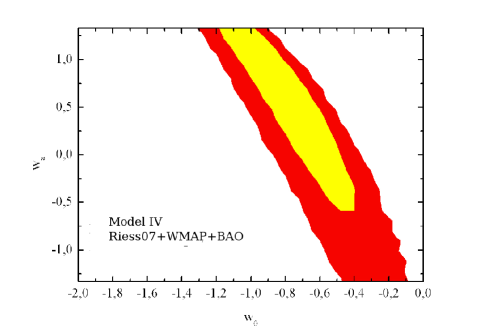
We consider different parametrizations of the dark energy equation of state parameter $w(z)$. The simplest model is the usual flat $\Lambda$CDM model with fixed equation of state $w=-1$ (MODEL I). We then let $w$ vary, assuming it is small enough to lead to acceleration. MODEL II has constant $w$ with a flat prior in the range $-1\leq\,w\leq\,-0.33$. In MODEL III, we expand the prior range to allow phantom dark energy models, constant $w$ with a flat prior $-2\leq\,w\leq\,-0.33$. We also consider dynamical dark energy models where $w$ can depend on redshift. In particular we consider a linear dependence on scale factor $a=(1+z)^{-1}$ as Chevallier & Polarski (2001):

$$w(a)=w_{0}+w_{a}(1-a)$$ (7)

with $-2\leq\,w_{0}\leq\,-0.33$ and $-1.33\leq\,w_{a}\leq\,1.33$ (MODEL IV). The above model is a low redshift approximation that may break at higher redshift. In this respect it is useful to include a more sophisticated parametrization that takes in to account the high redshift behaviour. We consider two possibilities. The first one is the one proposed by Hannestad and Mortsell (see Hannestad & Mortsell (2004)), where:

$$w(a)=w_{0}w_{1}\frac{a^{q}+a_{s}^{q}}{w_{1}a^{q}+w_{0}a_{s}^{q}}.$$ (8)

In this model (MODEL V), the equation of state changes from $w_{0}$ to $w_{1}$ around redshift $z_{s}=1-1/a_{s}$ with a gradient transition given by $q$. The priors are flat within $-2\leq\,w_{0}\leq\,0$, $-2\leq\,w_{1}\leq\,0$ and $0\leq\,q\leq\,10$.

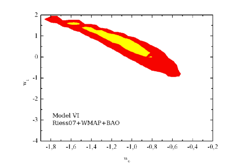
The second one is the parametrization introduced by Upadhye et al. (2005) where

$$w(z)=w_{0}+w_{1}z$$ (9)

for $z<1$ and

$$w(z)=w_{0}+w_{1}$$ (10)

for $z\geq 1$ (MODEL VI). In this case we choose flat priors in $-2\leq\,w_{0}\leq\,-0.2$ and $-4\leq\,w_{1}\leq\,2$. In analyzing each model, the priors for the other parameters are flat within the ranges
$0.1\leq\,\Omega_{m}\leq\,0.5$
$56\leq\,H_{0}/(km\,s^{-1}\,Mpc^{-1})\leq\,72$.

2.2 Cosmological Datasets

The dark energy models are then compared with the data following the approach described in Wang & Mukherjee (2004); Liddle et al. (2006b). In particular we compare the luminosity distance at redshift $z$ of each model given by

$$d_{L}(z)=c(1+z)\int_{0}^{z}\frac{dz^{\prime}}{H(z^{\prime})}$$ (11)

with the SN-Ia luminosity distances from the latest catalogue of Riess et al. (2007). This includes $182$ SN-Ia, “flux-averaged” with a $\Delta z=0.05$ binning as in Wang et al. (2005) to reduce possible systematic effects from weak lensing. We also consider the new $57$ supernovae coming from the ESSENCE Supernova Suvey of Wood-Vasey et al. (2007) in combination with the $38$ nearby supernovae (with $<0.023<z<0.15$) of Riess et al. (2007). We also consider the CMB shift parameter $R$ measured by the three-year WMAP experiment, $R=1.70\pm 0.03$ Spergel et al. (2006), in combination with the BAO measurement of the distance parameter at redshift $z=0.35$, $d_{V}(z=0.35)=1.300\pm 0.088$ Gpc (see Eisenstein et al. (2005)). The shift parameter $R$ is defined as

$$R=\Omega_{m}^{\frac{1}{2}}\int_{0}^{z_{CMB}}\frac{dz^{\prime}}{H(z^{\prime})},$$ (12)

where $z_{CMB}=1089$ is the redshift of recombination. For the BAO measurement, the distance parameter is:

$$d_{V}(z_{BAO})=\left[r^{2}(z_{BAO})\frac{cz_{BAO}}{H(z_{BAO})}\right]^{\frac{1}{3}}$$ (13)

where $r(z)$ is the comoving distance at redshift $z$ and $z_{BAO}=0.35$. We decide not to use data coming from weak gravitational lensing and galaxy clustering because they have the largest systematics and we prefer to be conservative in our analysis.

2.3 A new algorithm for computing Bayesian Evidence

Given a set of cosmological data, we evaluate the Bayesian Evidence by integrating the likelihood distribution with a method based on a modified version of the VEGAS algorithm. Introduced by Lepage (1978), VEGAS is widely used for multidimensional problems which occur in elementary particle physics. VEGAS is an importance-sampling algorithm, where regions where the integrand has large absolute value are sampled with a higher density of points than regions where it is low. The key element of the VEGAS algorithm is that samples are drawn from a probability distribution which is separable in the coordinates. This reduces complexity in two ways. In a $d$-dimensional problem, the probability distribution $p$ is specified by $d$ one-dimensional distributions, rather than one $d$-dimensional distribution:

$$p(\vec{\theta})\propto g_{1}(\theta_{1})g_{2}(\theta_{2})\ldots g_{d}(\theta_{d}).$$ (14)

Secondly, the generation of the samples is simplified by successively drawing from each of the $d$ probability distributions. The optimal weight function can be shown to be (Lepage, 1978)

$$g_{i}(\theta_{i})\propto\sqrt{\int_{j\neq i}d^{d-1}\theta_{j}\frac{f^{2}(\vec{\theta})}{\prod_{j\neq i}g_{j}(\theta_{j})}}$$ (15)

where $f(\vec{\theta})$ is the integrand to be sampled. An initial (e.g. random) sampling estimates $f$ roughly, from which an initial set $g_{i}$ can be constructed. Subsequent samples drawn from the $g_{i}$ can then be used to refine the $g_{i}$. See Press et al. (1986) for further details. A problem of VEGAS is that it may not do well when the integrand is concentrated in one-dimensional (or higher) curved trajectories (or hypersurfaces), unless these happen to be oriented close to the coordinate directions.

To solve this problem we have generalised the algorithm, and calculate, for a first and preliminary sampling, the covariance matrix of the Likelihood function. This we diagonalise and use the eigenvectors to define new parameters. In terms of these new parameters, the likelihood should be closer to separable. Note that this modified VEGAS algorithm should be particularly efficient if the likelihood is single-peaked. For multimodal likelihoods with more significant peaks, it will become increasingly less efficient, depending on the number, shape, relative height and orientation of the peaks.

Given a cosmological dataset and a theoretical framework, the Likelihood function will be clearly a function of $\vec{\theta}$:

$$L(\vec{\theta})\propto\,\exp\left[-\frac{\chi^{2}(\vec{\theta})}{2}\right]$$ (16)

and the algorithm calculates

$$I=\int\,d\vec{\theta}L(\vec{\theta}).$$ (17)

We always consider flat priors in our analysis; this implies that the priors will be constant so the Evidence will be given by:

$$E=P\cdot\,I,$$ (18)

where $P$ is simply the product of the various priors for the parameters, $P=\prod_{i=1}^{d}P_{i}$.

In the following we describe the principal steps of our algorithm:

• We do a first sampling of the likelihood function with $N_{COV}$ sampling points $\vec{\theta}$ and we calculate the covariance matrix $C=\langle\,(\vec{\theta}-\bar{\vec{\theta}})(\vec{\theta}-\bar{\vec{\theta}})^{T}\rangle$, which is symmetric and positive definite

• A square matrix which is symmetric and positive definite can be written as the product of a lower triangular and an upper triangular matrices (Cholesky decomposition):

  $$C=Q\cdot\,Q^{T}.$$ (19)

  We use the CHOLDC routine (seePress et al. (1986), par.$2.9$) to calculate the matrix $Q$. In general we can write the likelihood function as:

  $$L(\vec{\theta})\propto\,\exp\left(-\frac{1}{2}\vec{\theta^{T}}[C^{-1}]\vec{\theta}\right),$$ (20)

  where $C$ is the covariance matrix; if $\vec{y}=Q^{-1}\vec{\theta}$ we now have:

  $$L(\vec{y})\propto\,\exp\left(-\frac{1}{2}\vec{y}^{T}\vec{y}\right)$$ (21)

• We now choose to sample $\vec{y}$ rather than $\vec{\theta}$, so our sampling should be very efficient. In fact, most sampling points will be generated in the subspace of the parameter space where the likelihood function is not zero.

  It is clear that, changing our variables, the integral of the Likelihood will be given by:

  $$\int_{D}\,L(\vec{\theta})d\vec{\theta}=\int_{D^{\prime}}L(\vec{y})|\det(Q^{-1})|d\vec{y}.$$ (22)

  We perform $m$ statistically independent evaluations of the new function using $N$ sampling points for each iteration. The iterations are independent but they do assist each other because the algorithm uses each one to improve the sampling grid for the next one. The results of $m$ iterations are combined into a single best answer and its estimated error, by standard inverse variance weighting. We also compute $\chi^{2}$ to check that the best-fitting solutions are acceptable statistical fits.

Our results are clearly dependent on two parameters, the number $m$ of iterations and the number $N$ of sampling points for each iteration. The more iterations or sampling points are used, the more accuracy is reached. In Figures 1-2 we show how much the standard deviation depends on $m$ and $N$.

Figure 1: Standard deviation in function of the number of iterations $m$ used (with $N=5000$ for each iteration) in the calculation of the Likelihood function with $3$ parameters ($\Omega_{m},w,H_{0}$). The value of the integral is: $I=0.04915$

Figure 2: The same of Figure 1 but the standard deviation is plotted in function of the number N of sampling points (with $m=5$)

Figure 3: Density of sampling points in the $2$-dimensional space $\Omega_{m}-H_{0}$

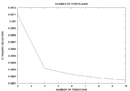
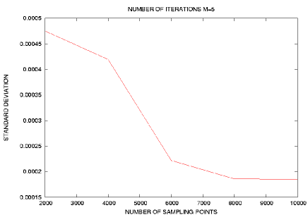
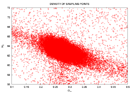
In Figure 3 we can see the density of sampling points in the $\Omega_{m}-H_{0}$ plane; the density will be greater in the subspace where the Likelihood function lives and we can also see the principal directions of the function. In general, implementing the routine for the calculation of the covariance matrix, the relative error $\frac{\sigma_{I}}{I}$ in the calculation of the integral is lowered by a factor $10$, for the same number of function evaluations. In our analysis we always use $m=5$ iterations and from $N=5000$ to $30000$ sampling points (depending on the dimension of the parameter space and on the size of the prior space), except for MODEL V for which $N=100000$. We reach an uncertainty of $\sim 10^{-3}$ in $\Delta\,\ln(E)$. We also used $N_{COV}=20000$ in the first iteration for calculating the covariance matrix: this large number is justified by the fact that it’s important to achieve a good estimate of the covariance matrix, to have good “principal directions” for the next samplings, especially when we handle with several parameters.

3 Results

Let us first analyze the full Riess et al. (2007) data in combination with CMB and BAO. The main results of this analysis are reported in Table 1 and in Figures $4$-$8$. The best-fitting parameter values are the means obtained from the full posterior probability distribution, rather than the maximum likelihood values. The standard deviations are similarly obtained from integration over the posterior.

Table 1: The parameter constraints together with the mean value of $\Delta\,\ln(E)$ and the minimum chisquared for the six models considered using the $182$ supernovae by Riess et al. 2007 Riess et al. (2007) binned with $\Delta\,z=0.05$ up to $z=1.7$ (about $34$ bins). The (unnormalized) $\ln(E)$ for the $\Lambda$CDM model is $\ln(E)=-16.2466\pm 0.0002$. The uncertainty in the value of $\Delta\,\ln(E)$ is calculated making use of the usual formula for the propagation of the uncertainty of a variable $x=x(\vec{y})\rightarrow\sigma_{x}=\sqrt{\sum_{i=1}^{N}\big{(}\frac{\partial\,x}{\partial\,y_{i}}\big{)}^{2}\sigma_{x_{i}}^{2}}$. In our case $\Delta\,\ln(E)=\ln(\frac{E_{1}}{E_{0}})\rightarrow\sigma_{\Delta\,\ln(E)}=\sqrt{\big{(}\frac{\sigma_{E_{0}}}{E_{0}}\big{)}^{2}+\big{(}\frac{\sigma_{E_{1}}}{E_{1}}\big{)}^{2}}$.

Constraints	$\Delta\,lnE$	$\chi^{2}_{Min}$	Model
$\Omega_{m}=0.28\pm 0.03$	0.0	24.39	I
$H_{0}=64.5\pm 0.09$
$\Omega_{m}=0.27\pm 0.03$	$-0.222\pm 0.005$	22.43	II
$H_{0}=63.4\pm 1.1$
$w<-0.84$ at $1\sigma$
$w<-0.73$ at $2\sigma$
$\Omega_{m}=0.27\pm 0.03$	$-1.027\pm 0.002$	22.43	III
$H_{0}=63.4\pm 1.1$
$w=-0.86\pm 0.1$
$\Omega_{m}=0.28\pm 0.04$	$-1.118\pm 0.015$	21.47	IV
$H_{0}=63.8\pm 1.4$
$w_{0}=-1.03\pm 0.25$
$w_{a}=0.76^{+--}_{-0.91}$
$\Omega_{m}=0.27\pm 0.03$	$-1.059\pm 0.008$	21.38	V
$H_{0}=63.5\pm 1.1$
$w_{0}=-0.85\pm 0.12$
$w_{1}=-0.81\pm 0.21$
$a_{s}$ unconstrained
$q$ unconstrained
$\Omega_{m}=0.30\pm 0.05$	$-1.834\pm 0.006$	21.52	VI
$H_{0}=63.5^{+1.8}_{-1.2}$
$w_{0}=-1.08_{-0.30}^{+0.24}$
$w_{1}=0.78_{-0.57}^{+0.83}$

Figure 4: Likelihood contours at $68\%$ and $95\%$ (two-parameter) for MODEL I

Figure 5: Likelihood contours at $68\%$ and $95\%$ for MODEL II

Figure 6: Likelihood contours at $68\%$ and $95\%$ for MODEL III

Figure 7: Likelihood contours at $68\%$ and $95\%$ for MODEL IV

Figure 8: Likelihood contours at $68\%$ and $95\%$ for MODEL VI

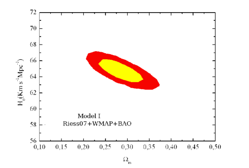
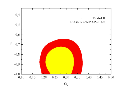
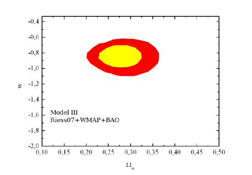
As we can see a cosmological constant is preferred by the data and is always compatible with it, independently of the model considered. The constraints we obtain on the equation of state parameter, assumed as a constant, are $w<-0.84$ in the case of $w\geq-1$ and $w=-0.86\pm 0.1$ at $68\%$ c.l. when models with $w<-1$ are included. Those constraints are compatible and of the same order of magnitude of the previous constraints reported by Liddle et al. (2006b) but where the new SN-Ia dataset of Riess et al. (2007) was not considered. However the evidence for the $w<-1$ case is worse by $\Delta\ln(E)\sim 1$, i.e. there is no indication from the data that we should extend the parameter space to these phantom dark energy models.

The same happens when we consider models with an equation of state parameter which varies with redshift.

For the models I-IV, which have the best Evidences and the same parametrization (with $w_{0}=-1$ and $w_{a}=0$ for MODEL I and $w_{a}=0$ for MODEL II-III) we have also considered results coming from the Bayesian model averaging; as explained in Liddle et al. (2006b), because of our ignorance about the true cosmological model, we may think that the probability distribution of the parameters is a superposition of its distributions in different models, weighted by the relative model probability, as in quantum mechanics, where the state of a physical system is a superposition of its possibilities until a measurement determines the collapse in a single eigenstate.

If we convert the $\Delta\,\ln(E)$ into posterior probabilities, assuming equal prior probabilities, we have $40.2\%$, $32.2\%$, $14.4\%$, $13.2\%$ for models I-II-III-IV.

The constraints on the cosmological parameters from the Bayesian model averaging of models I-II-III-IV are: $\Omega_{m}=0.27\pm 0.03$, $H_{0}=63.2^{+1.8}_{-1.2}$, $w_{0}=-1.0\pm 0.1$ at $1\sigma$, $w_{a}=0.0^{+0.02}_{-0.03}$ at $2\sigma$. The confidence limits in $w_{a}$ are exacly zero at $1\sigma$; this is because the probability distribution for this parameter is a delta function for models I-II-III and it is superimposed to the extended tails of model IV (as explained in Liddle et al. (2006b)).

It is also interesting to consider the effects on the cosmological parameters if we remove from the dataset the supernovae with $z>1$. In Table 2 we report our principal results.

Table 2: The parameter constraints together with the mean value of $\Delta\,\ln(E)$ and the minimum chisquared for the six models considered when $z<1$, using the $166$ supernovae with $z<1$ of Riess et al. $2007$ binned with $\Delta z=0.05$ (about $20$ bins).

Constraints	$\Delta\,lnE$	$\chi^{2}_{Min}$	Model
$\Omega_{m}=0.27\pm 0.04$	0.0	16.43	I
$H_{0}=64.6\pm 0.09$
$\Omega_{m}=0.27\pm 0.04$	$-0.223\pm 0.004$	14.54	II
$H_{0}=63.4\pm 1.3$
$w<-0.82$ at $1\sigma$
$w<-0.73$ at $2\sigma$
$\Omega_{m}=0.27\pm 0.04$	$-1.022\pm 0.004$	14.54	III
$H_{0}=63.4\pm 1.2$
$w=-0.86\pm 0.1$
$\Omega_{m}=0.29\pm 0.04$	$-1.090\pm 0.011$	13.33	IV
$H_{0}=63.6\pm 1.2$
$w_{0}=-0.98^{+0.26}_{-0.23}$
$w_{a}=0.72^{+--}_{-1.08}$
$\Omega_{m}=0.28\pm 0.04$	$-1.020\pm 0.008$	13.00	V
$H_{0}=63.4\pm 1.0$
$w_{0}=-0.88\pm 0.12$
$w_{1}=-0.63^{+0.2}_{-0.27}$
$a_{s}=$ (unconstrained)
$q=$ (unconstrained)
$\Omega_{m}=0.30\pm 0.05$	$-1.691\pm 0.01$	12.95	VI
$H_{0}=64.3\pm 1.2$
$w_{0}=-1.17\pm 0.37$
$w_{1}=$ (unconstrained)

As we can see, there are no significant differencies on the mean values however the error bars are generally reduced by a $\sim 30\%$. Models with varying-with redshift equation of state have a slightly better evidence but with a cosmological constant is still favoured.

It’s also useful to check if our results are the same when we consider a different dataset. To this extent, we use the $57$ supernovae coming from the ESSENCE Supernova Suvey Wood-Vasey et al. (2007) in combination with the $38$ nearby supernovae (with $0.023<z<0.15$) of Riess et al. 2007 (Riess et al. (2007)). We do not consider models with evolving dark energy, because in this analysis we limit our redshift range to $z<0.670$.

Table 3: Parameter constraints and Evidence for MODEL I-II-III, using the 95 supernovae of ESSENCE+nearby Riess et al. (2007) binned with $\Delta\,z=0.05$ up to $z=0.65$ ($15$ bins)

. Constraints $\Delta\,lnE$ $\chi^{2}_{Min}$ Model $\Omega_{m}=0.25\pm 0.04$ 0.0 10.73 I $H_{0}=64.7\pm 0.09$ $\Omega_{m}=0.27\pm 0.04$ $-0.258\pm 0.004$ 9.28 II $H_{0}=63.6\pm 1.3$ $w<-0.80$ at $1\sigma$ $w<-0.67$ at $2\sigma$ $\Omega_{m}=0.27\pm 0.04$ $-1.027\pm 0.003$ 9.28 III $H_{0}=63.5\pm 1.2$ $w=-0.86\pm 0.11$

The results are reported in Table 3. The results are fully compatible with those from the previous analysis and, again, they provide a substantial evidence for a constant $w$, with a cosmological constant being preferred.

4 Conclusions

In this paper we have carried out a Bayesian model selection analysis of several dark energy models using the new data of high redshift supernovae of Riess et al. 2007 (Riess et al. (2007)) and from the ESSENCE survey (Wood-Vasey et al. (2007)), together with Baryonic Acoustic Oscillations and Cosmic Microwave Background Anisotropies. To this extent, we have developed a new algorithm to calculate the Bayesian Evidence which is fast (less than $1$ hour for each calculation of the Evidence on a $2GHz$ CPU) and very accurate (a relative uncertainty $\frac{\sigma_{\Delta\,\ln(E)}}{\Delta_{\ln(E)}}<10^{-2}$ in $10^{5}$ likelihood evaluations).

We find that with current observational data the usual $\Lambda$CDM model is slightly preferred with respect to dark energy models with equations of state in the range $-1\leq\,w\leq 0$ and substantially preferred to dark energy models with $-2\leq\,w\leq 0$ or to dark energy models with an equation of state which evolves with time.

However we would like also to stress that it may be premature to reject models only on the basis of Bayesian model selection; in general, the simplest models may not be the “true” model. In this way, until we have a theoretical explanation of the accelerated expansion of the Universe, one should keep an open mind to all the alternatives to the $\Lambda$CDM scenario, even if, at the moment, it seems the simplest description of our Universe.

5 Acknowledgments

Paolo Serra thanks University of Edinburgh for support during his visit and members of the Royal Observatory of Edinburgh for their kind ospitality. We thank Andrew Liddle for useful comments.

References

- Alam (2006) U. Alam, V. Sahni and A. A. Starobinsky, arXiv:astro-ph/0612381, (2006).
- Astier et al. (2005) P. Astier et al., astro-ph/0510447, (2006).
- Barger et al. (2006) V. Barger, Y. Gao and D. Marfatia, arXiv:astro-ph/0611775, (2006).
- Bassett et al. (2004) B. A. Bassett, P. S. Corasaniti and M. Kunz, Astrophys. J. 617 (2004) L1 [arXiv:astro-ph/0407364].
- Chevallier & Polarski (2001) M. Chevallier and D. Polarski, Int. J. Mod. Phy. D., 10, 213 (2001)
- Dvali, Gabadadze, Porrati (2000) G. Dvali, G. Gabadadze and M. Porrati, Phys. Lett. B 485, 208 (2000).
- Efstathiou et al. (2002) G. P. Efstathiou et al., MNRAS, 348, L29 (2002).
- Eisenstein et al. (2005) D. Eisenstein et al., Astrophys. J. 633, 560 (2005).
- Elgaroy & Multamaki (2006) O. Elgaroy and T. Multamaki, JCAP 0609, 002 (2006) [arXiv:astro-ph/0603053].
- Giannantonio et al. (2006) T. Giannantonio et al., Phys. Rev. D 74 (2006) 063520 [arXiv:astro-ph/0607572].
- Gong and Wang (2006) Y. G. Gong and A. z. Wang, arXiv:astro-ph/0612196, (2006).
- Hannestad & Mortsell (2004) S. Hannestad and E. Mortsell, JCAP 0409 (2004) 001 [arXiv:astro-ph/0407259].
- Jarvis et al. (2005) M. Jarvis, B. Jain, G. Bernstein and D. Dolney, Astrophys. J. 644 (2006) 71 [arXiv:astro-ph/0502243].
- Jeffreys (1961) H. Jeffreys, “Theory of Probability”, Third edition, Oxford University Press (1961).
- Lepage (1978) G.P. Lepage, Journal of Computational Physics, 27, 192.
- Liddle et al. (2006a) A. Liddle, P. Mukherjee, D. Parkinson , A& G, 47, 4.30, 2006.
- Liddle et al. (2006b) A. R. Liddle, P. Mukherjee, D. Parkinson, Y. Wang, Pyhs. Rev. D., 74, 123506, (2006).
- Mukherjee, Parkinson, Liddle (2006) P. Mukherjee, D. Parkinson, A. R. Liddle, PpJL, 638, L51, (2006).
- Nesseris & Perivolaropoulos (2006) S. Nesseris and L. Perivolaropoulos, arXiv:astro-ph/0612653, (2006).
- Peebles & Ratra (2003) P. J. E. Peebles and B. Ratra, Rev.Mod.Phys. 75 (2003) 559-606 (2003).
- Perlmutter et al. (1999) S. Perlmutter et al. Astrophys. J. 517, 565 (1999), astro-ph/9812133.
- Press et al. (1986) W. H. Press, S. A. Teukolsky, W. T. Vetterling, B. P. Flannery “Numerical Recipes for Fortran 77: The Art of Scientific Computing” (Cambridge University Press, Cambridge, England, 1986).
- Riess et al. (1998) A. G. Riess et al. Astron. J. 116, 1009 (1998), astro-ph/9805201.
- Riess et al. (2004) A. G. Riess et al., Astrophys. J. 607, 665 (2004).
- Riess et al. (2007) A. G. Riess et al., arXiv:astro-ph/0611572.
- Sahni (2002) V. Sahni, Class. Quant. Grav. 19, 3435 (2002).
- Saini et al. (2004) V. Saini, J. Weller and S. Bridle, Mon. Roy. Astron. Soc. 348, 603 (2004)
- Szydlowski et al. (2006) M. Szydlowski, A. Kurek, A. Krawiec Phys.Lett. B642 (2006) 171 astro-ph/0604327
- Spergel et al. (2006) D. N. Spergel et al., astro-ph/0603449, (2006).
- Tegmark et al. (2006) M. Tegmark et al., astro-ph/0608632, (2006).
- Upadhye et al. (2005) A. Upadhye, M. Ishak and P. J. Steinhardt, Phys. Rev. D 72 (2005) 063501 [arXiv:astro-ph/0411803].
- Wang et al. (2005) Y. Wang and M. Tegmark, Phys. Rev. Lett. 92, 241302 (2004); Y. Wang, JCAP 03, 005 (2005).
- Wang (2000) Y. Wang, ApJ, 536, 531 (2000).
- Wang & Mukherjee (2004) Y. Wang, and P. Mukherjee, ApJ, 606, 654 (2004)
- Wang (2000) Y. Wang, Astrophys.J. 536 (2000) 531
- Wood-Vasey et al. (2007) W. M. Wood-Vasey et al., astro-ph/0701041, (2007).