Modelling Shock Heating in Cluster Mergers:
I. Moving Beyond the Spherical Accretion Model

Abstract

The thermal history of the intracluster medium (ICM) is complex. Heat input from cluster mergers, from AGN, and from winds in galaxies offsets and may even prevent the cooling of the ICM. Consequently, the processes that set the temperature and density structure of the ICM play a key role in determining how galaxies form. In this paper we focus on the heating of the intracluster medium during cluster mergers, with the eventual aim of incorporating this mechanism into semi-analytic models for galaxy formation.

We generate and examine a suite of non-radiative hydrodynamic simulations of mergers in which the initial temperature and density structure of the systems are set using realistic scaling laws. Our collisions cover a range of mass ratios and impact parameters, and consider both systems composed entirely of gas (these reduce the physical processes involved), and systems comprising a realistic mixture of gas and dark matter. We find that the heating of the ICM can be understood relatively simply by considering evolution of the gas entropy during the mergers. The increase in this quantity in our simulations closely corresponds to that predicted from scaling relations based on the increase in cluster mass.

We examine the physical processes that succeed in generating the entropy in order to understand why previous analytical approaches failed. We find that: (1) The energy that is thermalised during the collision greatly exceeds the kinetic energy available when the systems first touch. The smaller system penetrates deep into the gravitational potential before it is disrupted. (2) For systems with a large mass ratio, most of the energy is thermalised in the massive component. The heating of the smaller system is minor and its gas sinks to the centre of the final system. This contrasts with spherically symmetric analytical models in which accreted material is simply added to the outer radius of the system. (3) The bulk of the entropy generation occurs in two distinct episodes. The first episode occurs following the collision of the cores, when a large shock wave is generated that propagates outwards from the centre. This causes the combined system to expand rapidly and overshoot hydrostatic equilibrium. The second entropy generation episode occurs as this material is shock heated as it re-collapses. Both heating processes play an important role, contributing approximately equally to the final entropy. This revised model for entropy generation improves our physical understanding of cosmological gas simulations.

1 Introduction

The structure of the X-ray emitting gas that is seen in galaxy groups and clusters is still not understood. This gas (the intracluster medium, hereafter ICM) dominates the baryonic mass content of clusters and is material which is left over from galaxy formation. As such its properties present an important clue to the galaxy formation process. If the processes that set its temperature and density structure could be understood they should provide valuable constraints on galaxy formation models. However, linking together models for galaxy formation and accurate numerical methods capable of tracing the hydrodynamic evolution of the ICM has proved difficult. If cooling is neglected, the emission properties of clusters can be calculated in a robust manner (e.g., Evrard et al. 1996); however such simulations cannot form galaxies and thus omit a fundamental component of the physics. On the other hand, if cooling is included in the simulations, the results are not stable to changes in numerical resolution unless an effective form of heating is introduced to limit the cooling rate in small or early halos (e.g., Balogh et al. 2001; Borgani et al. 2006). Many different “feedback” mechanisms have been tried to oppose the cooling instability. Examples include galaxy winds and thermal energy injection (e.g., Springel & Hernquist 2003), delayed cooling (e.g., Kauffmann et al. 1999), preheating of intergalactic gas (e.g., Kaiser 1991; Evrard & Henry 1991), thermal conduction (e.g., Benson et al. 2003; Dolag et al. 2004), and heating by AGN (e.g., Dalla Vecchia et al. 2004; Sijacki & Springel 2006). These schemes have all met with various levels of success, but have not yet achieved a simultaneous match to the observed galaxy luminosity function, stellar mass fraction and temperature and density structure of the ICM. One factor slowing the development of these theoretical models is the lack of understanding of the physical processes at work in the simulations. Because it is so difficult to quantify the likely effect of introducing new processes, the models must be developed on a largely trial and error basis.

An alternative approach is to develop a semi-analytic model of the thermal history of the ICM, in which the complex physics is encapsulated in a small number of semi-empirical equations. This approach has been very successful in improving our understanding of galaxy formation (e.g., Cole et al 2000; Springel et al. 2005; Bower et al. 2006). The semi-analytic approach has been tried in several studies (e.g., Wu et al. 2000; Bower et al. 2001; Benson et al. 2003), but the results have been limited because the techniques for setting the gas distribution in the halos have been ad hoc. What is needed is to take a step back, and to better understand the results of simple gas hydrodynamic models. A better physical understanding of how entropy of the ICM is set in these simulations would equip us with the techniques needed to attack the much greater physical complexity of the problem when cooling and galaxy formation are included. This is the subject of this paper.

The starting point for the next generation of semi-analytical approaches to the ICM should be to describe the physical state of the gas in terms of its entropy distribution function. Entropy is a powerful concept for understanding the density and temperature structure of clusters, and was initially introduced as a means of quantifying the departures of cluster structures from the simple scalings expected for their mass and temperature distributions (Evrard & Henry 1991; Kaiser 1991; Bower 1997; Balogh et al. 1999; McCarthy et al. 2003). By knowing the entropy distribution of the gas, we can determine the density and temperature profiles of the ICM within a given dark matter gravitational potential (e.g., Voit et al. 2002). This process requires that an outer boundary condition is set (e.g. by computing the external pressure due to infalling gas) but the details of the boundary condition have only a weak effect on the profile. Discussing clusters in the language of entropy is extremely powerful, since the gas responds adiabatically to slow changes in the gravitational potential. Furthermore, the buoyancy of the ICM ensures that a relaxed system will have an ordered structure with the lowest entropy gas located in the deepest part of the gravitational potential. Only cooling and shock heating or mixing events alter the entropy distribution of the gas: cooling lowers the gas entropy, while shock heating and mixing can only raise it. Cooling in clusters is already well understood and can be modelled with simple semi-analytic techniques (e.g., McCarthy et al. 2004). However, we need to understand how entropy is generated during cluster growth to self-consistently model the cosmological formation of structure in a semi-analytic way.

So what sets the entropy distribution in clusters? Previous papers have looked at how entropy is generated in smoothly infalling gas (Cavaliere et al. 1998; Abadi et al. 2000; Tozzi & Norman 2001; Dos Santos & Doré 2002; Voit et al. 2003). For a spherically symmetric smooth shell, it is possible to determine the infall velocity and density of this material at the cluster virial radius. The bulk infall velocity is converted into internal thermal energy at a shock surrounding the cluster. The entropy generated in the shock can be computed from the Rankine-Hugoniot shock jump conditions. Modelling the growth of clusters in this way produces realistic entropy profiles, however the normalisation of the entropy is somewhat too high, so that the model predicts clusters with average densities $\rho_{\rm gas}$, that are lower than observed (see Voit et al. 2003).

However, the smooth accretion approximation is not valid in a cold dark matter (CDM) dominated universe since most of the mass accreted by clusters has previously collapsed into smaller virialised mass concentrations (e.g., Lacey & Cole 1993; Rowley et al. 2004; Cohn & White 2005). This leads to a problem for the picture above since the entropy generated drops rapidly if the accreted material is already dense and warm prior to the accretion shock. Importantly, if this deficit is present at every step in a system’s merger history, the problem becomes greatly compounded over time. This effect is far larger than the overestimate of the cluster entropy obtained in the smooth accretion case. Modelling a realistic structure in the accreted material leads to systems that are much denser and more luminous in X-rays than observed systems. This issue is discussed by Voit et al. (2003).

Recently, considerable progress has been made in simulating the growth of clusters using purely numerical techniques (e.g., Borgani et al. 2004; Kravtsov et al. 2005). The numerical simulations clearly show that $\rho_{\rm gas}\approx f_{b}\rho_{\rm tot}$ (where $f_{b}$ is the cosmic baryon fraction, and $\rho_{\rm tot}$ is total baryon + dark matter density) at large radii, in agreement with observations (e.g., Vikhlinin et al. 2006; McCarthy et al. 2007). This result holds for a wide range of simulation parameters and is largely insensitive to numerical technique or resolution (Frenk et al. 1999). The agreement between simulations and observations indicates that we do not yet have an adequate understanding of the lumpy accretion process, since analytic attempts to model this process yield results in strong discord with the observations. Our immediate aim is to improve our understanding of these simulations. Clearly, the approximate methods we wish to develop will not replace direct simulations, but they do provide an essential tool for understanding their results, for estimating the impact of limited numerical resolution, and for exploring the vast parameter space of heating mechanisms used in galaxy formation models. In subsequent papers, we will apply this understanding to improve the treatment of gas heating in semi-analytic codes galaxy formation models (e.g., Cole et al. 2000; Bower et al. 2006). By introducing our models for the shock heating of the ICM, we will be able to self-consistently model additional heating from supernovae and AGN. At present, the best efforts to track the impact of AGN heating in semi-analytic models (e.g., Bower et al. 2001) cannot follow properly the development of entropy and use an ad hoc description based on energy conservation.

In this paper we address the problem of lumpy accretion by focusing on idealised simulations of merging systems. We consider simple two-body collisions and explore how the entropy of the final system is generated. In setting up our two-body collisions, we remain as faithful as possible to the results of cosmological simulations. We initialise our systems with structural properties guided by the results of recent cosmological simulations and explore a wide range of representative mass ratios and orbits. These simulations show that the spherical accretion model previously considered is a poor representation of the true physical process in hierarchical cosmological models. We show that the kinetic energy of the infall lumps is much greater than previously estimated. Furthermore, we show that, if the mass ratio of the accretion event is large, only a small fraction of the kinetic energy is dissipated in the smaller component. Most of the heating effect is felt by the larger system. Our simulations allow us to present a much improved physical model for entropy generation in clusters.

The present paper is outlined as follows. In §2, we present the details of our simulation setup, including a discussion of the initial structural conditions of our systems, the adopted orbital parameters of the mergers, and other characteristics of the simulations. In §3, we analyse the entropy history of the systems during the merging process and qualitatively compare it with the standard spherical accretion model. In §4, we present an analytic model that encapsulates the essential physics of the merging process in our idealised simulations. Finally, in §5, we summarise and discuss our findings.

2 Simulation Setup and Methods

The baryons in virialised systems formed in non-radiative cosmological simulations approximately trace the dark matter with $\rho_{\rm gas}\approx f_{b}\rho_{\rm tot}$. Any reasonable model of shock heating ought to reproduce this basic result. However, as outlined in §1, it has so far proved quite difficult to construct a physical analytic model that can successfully pass this test. Exploration of idealised two-body mergers could provide the key insights necessary to achieve this goal. These idealised mergers should be representative of typical mergers in cosmological simulations and should themselves reproduce the propagation of (near) self-similarity. However, this is by no means a guaranteed result. First, idealised approaches such as those adopted below may be too simplistic to mimic closely enough the typical merger event in cosmological simulations. For example, the degree to which the self-similarity of systems formed in non-radiative cosmological simulations is sensitive to the exact initial conditions of the systems (i.e., structural properties) or to the properties of the merger orbits is unclear. There are few studies in the literature to date that examine the dependence of the properties of the baryons on the detailed merger history of a system. On the other hand, the adopted resolution of our idealised mergers is typically better than that of cosmological simulations. So it is possible that we may resolve phenomena that are not yet adequately resolved in cosmological simulations. In either case, the reproduction of self-similarity in our idealised simulations is not an automatic result. Below, we explore under what conditions self-similarity is achieved in our idealised merger simulations.

The following subsections present a description of our simulation setup and methods. This discussion goes into some detail and the reader who is mainly interested in the results of the simulations may wish to skip ahead to §3.

2.1 Initial conditions

We make use of the public version of the parallel TreeSPH code GADGET-2 (Springel 2005) for our merger simulations. The Lagrangian nature of this code makes it ideal for tracking the entropy evolution of specific sets of particles (or in principle even on a particle by particle basis) over the course of the simulations. By default the code implements the entropy-conserving SPH scheme of Springel & Hernquist (2002). This is ideal for our purposes since the code explicitly guarantees that the entropy of a gas particle will be conserved during any adiabatic process. Thus, we are assured that any increase in this quantity is rooted in physics.

We perform a series of binary merger simulations involving systems ranging in mass from $10^{14}M_{\odot}\leq M_{200}\leq 10^{15}M_{\odot}$ with the mass of the primary system (henceforth, we refer to the ‘primary’ system as the more massive of the two systems) in all collisions set by default to $M_{200}=10^{15}M_{\odot}$. ($M_{200}$ is defined in §2.1.1.) Thus, we simulate collisions characterised by mass ratios ranging from 10:1 to 1:1. Although we have experimented with a variety of mass ratios in this range, we present the results for simulations with mass ratios of 10:1, 3:1, and 1:1 only, but note that these yield representative results. Even though we have chosen to focus on the high end of the mass spectrum, the results should also be applicable to mergers involving lower mass systems (e.g., galaxies) so long as the mass ratio is similar. This is by virtue of the fact that gravity, which is scale-free, is completely driving the evolution of the systems. One of the reasons for choosing to focus on clusters is that gravitational processes dominate their final properties (X-ray observations demonstrate that non-gravitational processes such as cooling and AGN feedback influence the very central regions only of massive clusters; see, e.g., McCarthy et al. 2007). So we expect that our idealised merger simulations will be directly applicable to the bulk of the baryons in real clusters, although we leave a comparison with X-ray (and/or SZ effect) observations for future work. As outlined in §1, our primary goal is to develop a physical description of entropy generation in mergers.

2.1.1 Gas-only models

We have set up and run collisions of systems composed purely of gas. Of course, observations demonstrate that dark matter dominates by mass the baryons in galaxies, groups, and clusters and is of fundamental importance in the process of structure formation. In this respect, it might be expected that the gas-only merger simulations will have limited applicability. On the other hand, we anticipate that these idealised collisions will be considerably more straightforward to interpret than the gas + dark matter (hereafter, gas+DM) simulations (described below), given that the former have only a single phase to consider. If a physical understanding of the gas-only runs can be achieved then this could be quite helpful for understanding the role of dark matter in the combined runs. In fact, it is demonstrated in §3 that the gas+DM collisions exhibit what may be regarded as fairly minor deviations from the results of the gas-only runs. Thus, we find the gas-only simulations are potentially an excellent tool for elucidating the key physical processes in mergers of massive systems.

The systems are constructed to initially be structural copies of one another. In particular, the gas is assumed to have a NFW density profile (Navarro et al. 1997):

$$\rho(r)=\frac{\rho_{s}}{(r/r_{s})(1+r/r_{s})^{2}}$$ (1)

where $\rho_{s}=M_{s}/(4\pi r_{s}^{3})$ and

$$M_{s}=\frac{M_{200}}{\ln(1+r_{200}/r_{s})-(r_{200}/r_{s})/(1+r_{200}/r_{s})}.$$ (2)

In the above, $r_{200}$ is the radius within which the mean density is 200 times the critical density, $\rho_{\rm crit}$, and $M_{200}\equiv M(r_{200})=(4/3)\pi r_{200}^{3}\times 200\rho_{\rm crit}$.

To define the density profile for a halo of mass $M_{200}$, we must set the scale radius, $r_{s}$. The scale radius is often expressed in terms of a concentration parameter, $c_{200}\equiv r_{200}/r_{s}$. There are numerous studies that have examined the trend between concentration parameter and mass in pure dark matter cosmological simulations (e.g., Eke et al. 2001). The fact that there is a trend at all implies that the dark matter halos in these simulations are not strictly self-similar. But the mass dependence of the concentration parameter is weak, varying by only a factor of 2 or so from individual galaxies to galaxy clusters (with lower mass halos being more concentrated). A fixed concentration parameter of $c_{200}=4$, a value typical of galaxy clusters simulated in a $\Lambda$CDM concordance cosmology, is adopted for all of our systems.

In order to completely specify the properties of the gas we must choose an entropy profile and an outer boundary condition. As outlined in §1, the gas entropy is probably the most useful quantity to track during the simulations. In order to specify the entropy profiles of the systems, it is assumed that the gas is initially in hydrostatic equilibrium:

$$\frac{dP(r)}{dr}=-\frac{GM(r)}{r^{2}}\rho_{\rm gas}(r)$$ (3)

The entropy, $K$, is then deduced through the equation of state $P=K\rho_{\rm gas}^{5/3}$. A boundary condition must be supplied before equation (3) can be solved and we specify a value for the pressure of the gas at $r_{200}$, where we truncate the gas profiles (unless stated otherwise). There is some freedom in our choice of the pressure at the edge of the system. However, for physically reasonable values of $P(r_{200})$ there is in fact very little difference between the resulting profiles. For the bulk of the gas, we find that the requirement of hydrostatic equilibrium forces $K(M_{\rm gas})$ into a near power-law distribution with an index of approximately 1.3. This can be understood by noting that at intermediate radii the NFW profile is approximated well by an isothermal profile (i.e., $\rho\propto r^{-2}$), which has an entropy profile characterised by $d\log{K}/d\log{M_{\rm gas}}=4/3$. To ensure that our initial systems are structural copies of one another and to ease the comparison between the initial and final systems later on, a value of $P(r_{200})$ that establishes this near pure power-law entropy distribution all the way out to the system’s edge is selected. In real systems, the hot diffuse baryons are supposedly confined by the ram pressure of infalling material. Experimenting with a physical model for this ram pressure, Voit et al. (2002) have demonstrated that groups and clusters are indeed expected to have near power-law entropy distributions out to large radii.

The analytic profiles must be discretised into individual particles for input into the GADGET-2 code. In particular, the initial particle positions, velocities, and internal energies (per unit mass) must be specified.

For the initial particle positions, we start by generating a glass using the “MAKEGLASS” compiler option of GADGET-2. Basically, a Poisson distribution of particles is generated and is then run with GADGET-2 using $-G$ in place of $G$ for Newton’s constant. We allow the simulation to run for $\approx$1000 time steps to ensure the glass achieves a uniform distribution. This uniform distribution is then morphed into the mass profile that corresponds to the density profile given in equation (1). This is done by selecting a point inside the distribution of particles, which we have taken to be the centre of mass, ranking all of the particles according to the distance from this point, and then moving each particle radially such that the desired mass profile is achieved.

For the particle velocities, the baryons are initially assumed to be at rest in their hydrostatic configuration.

The specific internal energy, $I$, defined as $I=(3/2)P/\rho_{\rm gas}$, of each particle is assigned by using the particle’s distance from the centre of the halo and interpolating within the analytic profiles derived above.

Lastly, we surround the systems with a low density medium with a pressure set to $P(r_{200})$. This medium is dynamically-negligible and is simply put in place to confine the gas particles near the system’s edge. Without a confining medium as much as 20% of the system’s mass can leak beyond $r_{200}$.

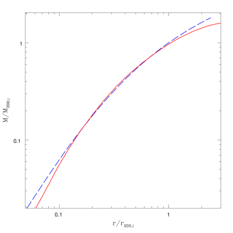
Figure 1: Testing the local Maxwellian approximation for the primary system. The dashed blue curve shows the initial mass profile extended out to $r_{25}$. The solid red curve shows the resulting equilibrium mass profile after running the dark matter halo in isolation for 50 Gyr (i.e., many dynamical times). Over the range the $0.1\leq r/r_{200}\leq 1.0$ the initial and final mass profiles follow each other closely.

2.1.2 Gas + dark matter (gas+DM) models

For the systems containing both gas and dark matter a slightly different procedure is used to construct the systems. First, we set up systems composed entirely of dark matter. The density profiles of the systems are given by equation (1). However, for reasons described below, we extend the dark matter well beyond $r_{200}$, to an overdensity of 25 (for our adopted concentration $r_{25}\approx 2.44r_{200}$). As in the gas-only setup, a glass particle distribution is morphed into the desired mass profile. Unlike the gas, however, the dark matter particles have no thermal pressure and must be assigned appropriate velocities in order to maintain this mass profile. To achieve this, we solve the the Jeans equation (see Binney & Tremaine 1987):

$$\frac{d[\sigma^{2}_{r}(r)\rho(r)]}{dr}=-\frac{GM(r)}{r^{2}}\rho(r)$$ (4)

for the velocity dispersion profile, $\sigma_{r}(r)$, of the systems. Equation (4) implicitly assumes that the orbits of the dark matter particles are purely isotropic.

To solve equation (4) it is assumed that virial equilibrium holds at the edge of the dark matter halo (see, e.g., Ricker & Sarazin 2001); i.e.,

$$\sigma_{r}(r_{25})=\sqrt{\frac{GM_{25}}{3r_{25}}}$$ (5)

We have also experimented with the boundary condition that $\sigma^{2}_{r}(r)\rho(r)\rightarrow 0$ as $r\rightarrow\infty$ and obtained very similar results within $r_{25}$. Henceforth, results are presented for the runs that make use of the boundary condition given by equation (5).

Each of the three velocity components for a dark matter particle are assigned a random value picked from a Gaussian distribution with width equal to the 1-D velocity dispersion, $\sigma_{r}$, at that radius. However, it is known that this local Maxwellian approximation does not result in a system that is initially in equilibrium (though it is not far removed from one). Of most concern is that a sharp truncation of the system at some finite radius results in a significant amount of the mass near this radius seeping out to much larger distance. Thus, the resulting equilibrium mass profile can be significantly different from that which was originally intended. In fact, this happens at all radii but in the system’s interior the flux of particles moving to larger radii is offset by particles moving inwards (which were originally at larger radii). This obviously cannot happen near the system’s edge where there are no particles originally at larger radii (and moving inwards) to replace those moving away from the system’s centre. One way to overcome this problem is to apply a smooth tapering of the density profile beyond the system’s edge and compute the distribution function of the particles as opposed to making the Maxwellian assumption (e.g., Kazantzidis et al. 2004; Poole et al. 2006). However, we adopt a more simplistic, but still effective, method for overcoming this problem. In particular, as mentioned above, the initial dark matter profile is extended well beyond $r_{200}$, out to $r_{25}$. The aim is to ensure that within $r_{200}$, our region of interest, there is a large enough influx of particles to maintain the desired mass profile.

The pure dark matter halos are run in isolation for many dynamical times. In Figure 1, we show that by extending the dark matter halo out to $r_{25}$, the resulting equilibrium mass profile for the primary system traces the initial (intended) profile within $r_{200}$ quite well. A slight deviation is apparent for $r<0.1r_{200}$, which is due to limited mass resolution. However, we explicitly demonstrate in the Appendix that this deviation has negligible consequences for our equal mass mergers. In the case of our unequal mass mergers, the secondary systems are resolved with fewer particles and therefore the deviation at small radii is slightly larger in these systems. However, as we demonstrate in §4.2 and discuss further in the Appendix, the vast bulk of the energy is thermalised in the more massive primary system. So, as long as the primary system is well resolved the properties of the final merged system should be robust. This is what likely accounts for the fact that the properties of massive virialised systems formed in non-radiative cosmological simulations are robust to relatively large changes in numerical resolution (see, e.g., Frenk et al. 1999).

A drawback of extending the halo out to much larger radii is that a significant fraction of the mass is located outside the region of interest (thus, we potentially waste a good deal of computational effort). In order to mitigate this issue, we take the equilibrium configuration after running the dark halos in isolation and simply clip particles that lie beyond $r_{50}$. We have run the clipped halos for a further 10 Gyr and verify that the mass profiles within $r_{200}$ is virtually unaffected. This clipped equilibrium configuration is used to set up our initial gas+DM systems. We keep the current positions and velocities for our initial values for the dark matter particles in the combined runs. For the gas particles we also use the positions of the dark matter particles (that is, for those particles that lie within $r_{200}$) but reflect them through the centre of mass so that the gas particles do not lie directly on top of the dark matter particles. The gas particle velocities are set to zero and the internal energy densities are determined by placing the gas in hydrostatic equilibrium within the total gravitational potential. As in the gas-only models described above, a pressure boundary condition is selected such that $K(M_{\rm gas})$ is nearly a pure power-law out to $r_{200}$.

The above procedure implies that we will have equal numbers of gas and dark matter particles in our combined runs within $r_{200}$ (i.e., double the number of particles used in the isolated dark matter run within that radius). In order to conserve mass, so that the equilibrium state for the dark matter is still valid, we re-assign the dark matter particle masses to $(1-f_{b})$ times that used in the isolated run while the gas particles are assigned a mass of $f_{b}$ times the dark matter particle mass in the isolated run. Here $f_{b}$ is the ratio of gas mass to total mass within $r_{200}$, which is set to the universal value of $\Omega_{b}/\Omega_{m}=0.02h^{-2}/0.3=0.136$.

The end result of the above procedure is that the gas traces the dark matter, both phases are initially in equilibrium, and within $r_{200}$ both phases have a form that is very nearly the intended NFW distribution. As in the gas-only models, we surround the gas+DM systems with a low density pressure-confining gaseous medium.

2.2 Merger orbits and other simulation characteristics

We follow the approach of Poole et al. (2006) and use the results of cosmological simulations to help specify the orbital properties of our idealised merger simulations. In particular, we turn to the study of Benson (2005; but see also Tormen 1997; Vitvitska et al. 2002; Wang et al. 2005; Khochfar & Burkert 2006). Benson (2005) used a large collection of N-body simulations carried out by the VIRGO Consortium to study the distribution of orbital parameters of substructure falling onto massive (primary) halos. Particular emphasis was given to the 2-D distribution of the relative radial and tangential velocities of the substructure as they passed through a spherical shell with a radius set to $r=(1\pm 0.2)r_{\rm vir}$, where $r_{\rm vir}$ is the virial radius of the primary halo. As anticipated, the peak of the distribution corresponds to approximately the circular velocity of the primary halo at the virial radius (see his Fig. 2). In particular, $v\equiv(v_{r}^{2}+v_{t}^{2})^{1/2}\approx 1.1v_{c}(r_{\rm vir})$, where $v_{r}$ and $v_{t}$ are the relative radial and tangential velocities, respectively. For the individual components, the peak of the distribution is approximately centred on $v_{r}\approx 0.9v_{c}(r_{\rm vir})$ and $v_{t}\approx 0.65v_{c}(r_{\rm vir})$ and it is clear that there is a correlation between $v_{r}$ and $v_{t}$. However, as pointed out by Benson (2005), the centring of the peak also depends on the total mass of systems (see his Fig. 4). In particular, the orbits of mergers involving massive systems are more radial and less tangential than those of mergers involving low mass halos, presumably because more massive structures tend to form at the intersections of large-scale filaments. Unfortunately, the sample wasn’t large enough to fully quantify this mass dependence.

For the purposes of the present study, we adopt the following set of orbital parameters, which are representative of the results of Benson (2005). Unless stated otherwise, a fixed relative total velocity corresponding to the circular velocity of the primary at $r_{200}$, $\approx 1444$ km/s, is adopted initially for all of our simulations. This is slightly lower than the mean value found by Benson (2005), but consistent at the 1-sigma level. For the gas+DM simulations, we examine three different orbits for each mass ratio, corresponding to $v_{t}=0$, $v_{t}=v_{r}/4$, and $v_{t}=v_{r}/2$. We refer to these as the “head on”, “small impact parameter” and “large impact parameter” runs, respectively. In practical terms, this implies $v_{t}\approx 0.243v_{c,p}(r_{200})$ and $v_{t}\approx 0.447v_{c,p}(r_{200})$ for the latter two. This choice spans the lower half of the $v_{t}/v_{r}$ distribution for massive halos seen in Fig. 4 of Benson (2005). For the gas-only simulations, which we run simply to help coax out the key physics during mergers, we simulate head on collisions only [i.e., $v_{r}=v_{c,p}(r_{200})$ and $v_{t}=0$].

Table 1: Merger Orbital Parameters.

Mass ratio	Sim. type	$d_{0}$	$v_{r}$	$v_{t}$
		(kpc)	(km/s)	(km/s)
1:1	gas-only	4126	1444	0
3:1	gas-only	3494	1444	0
10:1	gas-only	3021	1444	0
1:1	gas+DM	4342	1444	0
1:1	gas+DM	4342	1400.9	350.2
1:1	gas+DM	4342	1291.6	645.8
3:1	gas+DM	3658	1444	0
3:1	gas+DM	3658	1400.9	350.2
3:1	gas+DM	3658	1291.6	645.8
10:1	gas+DM	3170	1444	0
10:1	gas+DM	3170	1400.9	350.2
10:1	gas+DM	3170	1291.6	645.8

Each of the simulations are initialised with the gaseous components of the primary and secondary systems just barely touching. Thus, the initial separation, $d_{0}$, is just the summation of $r_{200}$ for the primary and $r_{200}$ for the secondary. For the gas+DM simulations, this implies that there is initially some overlap of dark matter halos of the primary and secondary systems, which extends beyond the gaseous component. A complete summary of the adopted orbital parameters of all of our simulations is presented in Table 1. Note that for a fixed mass ratio $d_{0}$ differs slightly between the gas+DM and the gas-only simulations. This difference arises owing to the slight deviation of the mass profiles in the gas+DM simulations from the intended NFW distribution. Finally, the simulations have been set up such that the physical and centre-of-mass (of the entire system) coordinates and velocities are identical, where we have approximated the initial configuration as two point masses.

We have carried out a mass resolution study of one of our simulations (see the Appendix). Based on this study we adopt the following conditions. The primary systems in our default runs have 50,000 gas particles within $r_{200}$. This is the case for both the gas-only and gas+DM runs and implies the gas particle mass is $2\times 10^{10}M_{\odot}$ in the former and $f_{b}(2\times 10^{10}M_{\odot})=0.272\times 10^{10}M_{\odot}$ in the latter. In the gas+DM runs, the primary systems have $\approx$76,500 dark matter particles within $r_{50}$ and 50,000 within $r_{200}$ with a dark matter particle mass of $(1-f_{b})(2\times 10^{10}M_{\odot})=1.728\times 10^{10}M_{\odot}$. These particle masses are held fixed for the secondary systems as well (thus, they contain fewer particles than the primary).

For the gravitational softening length, we adopt a fixed physical size of 10 kpc for both the gas and dark matter particles. (We have also experimented with softening lengths of 5 kpc and 20 kpc and found the differences in the entropy evolution to be negligible.) We use a fairly standard set of SPH parameters, including a viscosity parameter, $\alpha_{\rm visc}$, of 0.8, a Courant coefficient of 0.1, and the number of SPH smoothing neighbours, $N_{\rm sph}$, is set to $50\pm 2$.

Finally, each simulation is run for a duration of 13 Gyr, i.e., approximately a Hubble time. Particle data is written out in regularly spaced intervals of 0.1 Gyr.

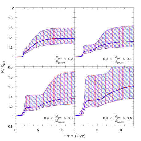
Figure 2: Entropy evolution in the 1:1 gas-only merger. The red and blue lines/hatched regions represent the primary and secondary systems, respectively. The upper and lower bounds of the hatched regions represent the 75^th and 25^th percentiles, respectively, while the central (thick) lines represent the median. The panels show the evolution of the entropy of particles separated according to their initial position in the cumulative gas mass profile. Since the cumulative gas mass profile is a monotonic function of radius, the panels also separate the particles according to initial distance from the centre of their respective halos.

3 Simulation Results

Below we present a detailed discussion of the entropy evolution of our simulations. The reader who is mainly interested in a general understanding of this progression may wish to skip ahead to §3.3, which presents a summary of our findings.

3.1 Gas-only simulations

3.1.1 Entropy evolution

We start by considering the evolution of the entropy in the gas-only merger simulations. Plotted in Figure 2 is the evolution for the 1:1 merger subdivided into spherical shells. Immediately apparent is the high degree of symmetry in the 1:1 merger. In all four regions the 25^th, 50^th, and 75^th percentiles follow each other quite closely. In addition, with the exception of the outermost ring, it is evident that the particles in both systems have achieved a nearly convergent state by the end of the simulation. Of course, it is possible to continue running the simulation to determine exactly what the convergent state of the outermost regions will be. However, since we have already run the simulation for a Hubble time this implies that the outer regions of systems formed from similar mergers in cosmological simulations will also not have had sufficient time to completely virialise by the present day. Since one of our aims is to understand the results of such simulations, we limit the duration of our simulations to 13 Gyr. Below we will compare this final configuration with a scaled up copy of the initial systems.

Some discussion of how the particles in each system actually get their entropy is warranted. To help aid the discussion we plot in Fig. 3 a sequence of snapshots of the 1:1 merger with particles colour coded according to the fractional change in entropy since the previous simulation output. The general progression of the merger can be described as follows. Since the two systems are initially just barely touching and have a relative velocity of $v_{c,p}(r_{200})$, they begin interacting as soon as the simulation starts. In particular, two large shock fronts are quickly established as the systems approach one another (see the panel corresponding to $t=1$ Gyr in Fig. 3). However, there is very little increase in the entropy of the particles in any of the four regions plotted in Fig. 2 until after the cores of the two systems collide at $t\approx 2$ Gyr into the simulation. The implication is that the initial shocks are actually quite weak (as the colour coding in Fig. 3 would also indicate). A plausible explanation for this behaviour comes when one compares the sound speed of the gas, $c_{s}$, defined as

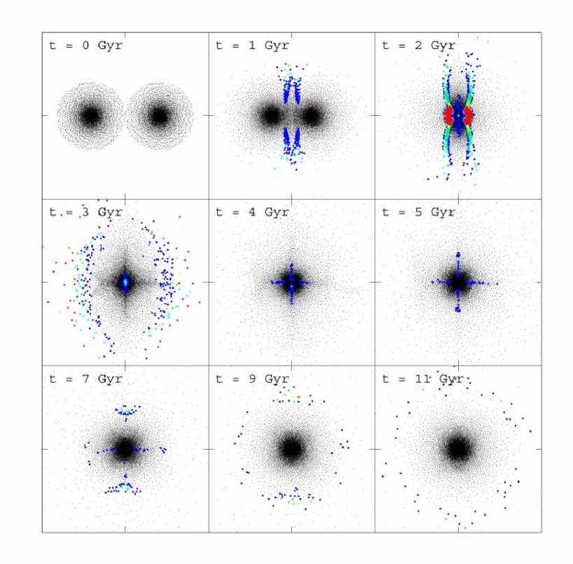
Figure 3: Fractional change in particle entropy as a function of time for the 1:1 gas-only merger. Shown are particles in a slice through the centre of thickness 250 kpc (i.e., $|z|<125$ kpc). Particles are colour coded according to the fractional change in entropy since the last simulation output (0.1 Gyr ago). Black points are for a fractional change of less than 2%, blue are for a 2%-10% change, cyan are for a 10%-20% change, green are for a 20%-30% change, yellow are for a 30%-40% change, and red are for a $>$ 40% change. For clarity the surrounding pressure-confining medium is not displayed. Each panel is 10 Mpc on a side.

$$c_{s}\equiv\sqrt{\frac{\partial P}{\partial\rho}}=\sqrt{\frac{\gamma P}{\rho}}=\sqrt{\frac{5}{3}\frac{k_{b}T}{\mu m_{p}}}$$ (6)

with the initial relative velocity of the merger. Since the initial relative velocity of the merger is set to the circular velocity, we are effectively comparing the sound crossing time of a system with its dynamical time. The condition of hydrostatic equilibrium ensures that the gas temperature will be such that these two timescales are comparable. In this case we find the mean sound speed of the systems is $\approx$1200 km/s. Compared to the initial relative velocity (see Table 1), this implies an initial Mach number of only $\cal{M}\approx$ 1.2. Therefore, we should expect only mild shock heating to occur during the early stages of the merger (as observed in Fig. 2). However, as we illustrate in §4, by the time the cores collide the relative velocity can approach or exceed nearly 3 times the initial value, effectively bringing the merger into the strong shock regime.

Following the collision of the cores, a large shock wave is generated. This shock quickly propagates outwards, heating the gas that was initially predominantly on the far side of each system and has not yet finished falling in (see the panels corresponding to $t=2$ and 3 Gyr in Fig. 3). In fact, this shock wave, combined with the expansion of the shocked high pressure/density gas near the core of the merged system, succeeds in reversing the infall of the material. This outflow of gas proceeds nearly adiabatically for a period of time that is dictated by the initial distance of the particle from its system’s centre. For example, for the outermost ring plotted in Fig. 2 this period of adiabatic expansion occurs from $t\approx 2.5$ Gyr for a duration of nearly 3.5 Gyr. Gas particles initially located close to the centre of their respective system do not spend such a large time in this outflow phase, as they end up being more deeply embedded within in the merged system’s potential well.

Figure 4: Entropy evolution in the 3:1 (left) and 10:1 (right) gas only mergers. The red and blue lines/hatched regions represent the primary and secondary systems, respectively. The upper and lower bounds of the hatched regions represent the 75^th and 25^th percentiles, respectively, while the central (thick) curves represent the median. The panels show the evolution of the entropy of particles separated according to their initial position in the cumulative gas mass profile. Since the cumulative gas mass profile is a monotonic function of radius, the panels also separate the particles according to initial distance from the centre of their respective halos.

The outflowing gas eventually halts and begins to re-accrete onto the core of the merged system. Although the gas accretes from virtually all directions, the symmetry of the 1:1 merger is such that the accretion happens preferentially along and perpendicular to the original collisional axis. This occurs for a significant period of time, until the merged core has achieved a near spherical symmetry. Following this, gas continues to accrete at the outskirts of the system but does so in a more or less spherical fashion. As evidenced from Figs. 2 and 3, the gas is slowly being shock heated during this period of re-accretion. The character of this episode of entropy production therefore differs significantly from the first abrupt episode following core collision. However, as Fig. 2 indicates, both episodes are of comparable importance in terms of setting the final state of the gas. Finally, we note that the late time (nearly spherical) accretion of material is what gives rise physically to the continued increase of entropy in the outermost regions of the system until the end of the simulations (e.g., as in the bottom-right panel of Fig. 2).

An interesting question is whether or not much mixing occurs as a result of the merging process. We have tested this by tracking not only the entropy evolution of individual particles but also their spatial distributions. Interestingly, even though the shock heating of the systems occurs in an “inside-out” fashion, we see very little evidence for mixing. For example, particles that were initially located near the centres of the two (pre-merger) halos (i.e., particles that initially have relatively low entropies) end up being located near the centre of the final merged system, whereas the large-radii (high entropy) particles end up occupying the outer regions of the final system. A plausible explanation for this behaviour is that the initial Mach number distribution of the particles varies relatively weakly with radius. This can be understood by considering the initial temperature profiles. The condition of hydrostatic equilibrium results in initial temperature profiles that vary by less than a factor of 2 from the cluster centre to its periphery. This then implies the Mach number distribution varies by less than a factor of $2^{1/2}$ over the entire system. Therefore, to a large degree, one expects (and the simulations bear this out) that most of the particles will be shock heated to a similar degree. As a result, convective mixing is minimal. This agrees well with the idealised cluster merger simulations of Poole et al. (2006).

The entropy evolution of the 3:1 and 10:1 gas-only mergers is plotted in Figures 4a and 4b, respectively. In a qualitative sense, both the primary and secondary systems in these mergers behave in a similar manner to the systems in the 1:1 case. For example, they both generate two relatively weak shock fronts early on, with the secondary driving a bow shock into the primary and vice-versa. As in the 1:1 case, they exhibit two main periods of entropy production, the first being associated with a strong shock approximately when their cores collide and the second being associated with an extended period of re-accretion shocks. Furthermore, we also see little evidence for mixing in the 3:1 and 10:1 mergers. Of course there are some differences between the three sets of simulations in detail. For example, because the sound speed of the gas in the secondary in the 10:1 collision is smaller than that in the 1:1 case, the initial Mach number for the secondary is higher. Consequently, the initial bout of shock heating before the cores collide is relatively more important for the secondary in high mass ratio mergers.

Figure 5: Comparison of the resulting entropy distributions from the 1:1 gas-only merger with self-similar expectations. Left: Comparison of radial profiles. The short-dashed red curve represents the initial entropy profile of the primary, the long-dashed magenta curve represents a self-similarly scaled up version of this profile, and the solid green curve represents the final entropy profile of the total merged system. Right: Comparison of Lagrangian gas mass profiles. The short-dashed red, long-dashed blue, and solid green curves represent the final $K(M_{\rm gas})$ distributions of the primary, secondary, and total merged systems, respectively. The horizontal dotted line represents the self-similar scaling.

It is clear from a comparison of Figs. 2 and 4a,b that the higher the mass ratio of the merger the more strongly heated the secondary is relative to the primary. This again may be tied to the fact that as one decreases the mass of the secondary its characteristic temperature decreases resulting in a decreased sound speed and an increased Mach number. It is also expected if the preservation of self-similarity is achieved by heating both the secondary and the primary up to same level. To explain, $K=P/\rho_{\rm gas}^{5/3}\propto T/\rho_{\rm gas}^{2/3}$, but self-similarity means that all systems have the same internal mass structure and therefore the characteristic entropy depends only on the temperature of the system. The virial theorem relates the temperature of a system with its mass via $M\propto T^{3/2}$, and therefore the characteristic entropy of a system scales simply as

$$K\propto M^{2/3}$$ (7)

Initially, therefore, the ratio of the secondary’s characteristic entropy to that of the primary is $K_{s}/K_{p}=(M_{s}/M_{p})^{2/3}$. So the secondary requires extra heating to overcome its initial deficit compared to the primary if self-similarity is achieved by heating both systems to the same level.

3.1.2 Final configurations

How do the final entropy distributions of the gas-only mergers compare with self-similar expectations? Figure 5 presents this comparison for the 1:1 gas-only merger both in traditional radial coordinates (left panel) and in physical gas mass coordinates (right panel). In Figure 5a, we compare the initial entropy radial profile of the primary system with the final radial profile of the total merged system. We also show a self-similarly scaled up version of the primary’s initial entropy profile, achieved by scaling the entropy coordinate up by $(M_{\rm tot}/M_{p})^{2/3}=2^{2/3}$ and the radial coordinate by $(M_{\rm tot}/M_{p})^{1/3}=2^{1/3}$. Fig. 5a shows that the scaled up version of the primary’s initial entropy profile follows the final entropy profile of the merged system over approximately two decades in radius. This indicates that, by and large, the 1:1 gas-only merger has scaled self-similarly through the merger. However, deviations are clearly visible, particularly at large radii. These are discussed in more detail below.

Figure 6: Comparison of the resulting $K(M_{\rm gas})$ distributions from the 3:1 (left panel) and 10:1 (right panel) gas-only merger with self-similar expectations. The short-dashed red, long-dashed blue, and solid green curves represent the primary, secondary, and total systems, respectively. The horizontal dotted line represents the self-similar scaling.

The entropy distributions of observed systems are most commonly presented in radial coordinates (e.g., Piffaretti et al. 2005; Donahue et al. 2006; Pratt et al. 2006), and so it is useful to present theoretical models in such units if the goal is to explain the properties of observed systems. However, our immediate goal in this paper is to develop a physical shock heating model. For this purpose, the entropy distributions are best presented in Lagrangian (gas mass) coordinates. In Figure 5b, therefore, we plot the final $K(M_{\rm gas})$ distributions for the merged system and for the primary and secondary individually for the 1:1 gas-only merger. The gas mass coordinate has been normalised by the total gas mass in the systems (in this case $10^{15}M_{\odot}$ for the primary and secondary and $2\times 10^{15}M_{\odot}$ for the final merged system). The entropy coordinate has been scaled to the self-similar expectations; i.e., the initial $K(M_{\rm gas})$ distribution of the primary scaled up by a factor of $(M_{\rm tot}/M_{p})^{2/3}$. (Equivalently, we could use the initial entropy distribution of the secondary scaled up by a factor of $[M_{\rm tot}/M_{s}]^{2/3}$.) Perhaps the simplest way to achieve this state is by having the primary and secondary systems individually obey self-similarity following the merger. In this case, we would expect the final distribution of the particles belonging to the primary to be $(M_{\rm tot}/M_{p})^{2/3}$ times the initial distribution, while the secondary’s final distribution would be a factor of $(M_{\rm tot}/M_{s})^{2/3}$ larger than its initial distribution.

If self-similarity is strictly obeyed, then the solid green curve in Figure 5b, which represents the final $K(M_{\rm gas})$ distribution for the merged system, should lie on the horizontal dotted line. Fig. 5b shows that, without any fine tuning of the simulations, the central 80% of the gas mass of the final merged system lies within approximately 10% of the self-similar result. As expected, the symmetry of the 1:1 case is such that both the primary and secondary individually obey self-similarity as well.

Beyond $M_{\rm gas}/M_{\rm gas,tot}\approx 0.8$ or so there is an apparent entropy excess relative to the self-similar expectation. Below, in §3.1.3, we demonstrate that this effect is artificial and its origin can be attributed to the (unrealistic) abrupt truncation of the gaseous atmospheres of our idealised systems at $r_{200}$. Fortunately, as demonstrated below, this effect is limited to the outermost regions of our systems only.

The $K(M_{\rm gas})$ distributions for the 3:1 and 10:1 gas-only mergers are plotted in Figures 6a and 6b, respectively. In both cases the final merged system is quite close to the self-similar result for the central $\sim 70$% of gas mass. Beyond this the edge effect discussed below kicks in. Thus, the 3:1 and 10:1 cases both qualitatively and quantitatively resemble the 1:1 case. Interestingly, however, the path through which the final merged systems in the 3:1 and 10:1 cases achieve self-similarity is by over-heating the primary and under-heating the secondary, not by both obeying self-similarity individually. This implies that some of the infall energy initially associated with the secondary system went into thermalising the gas of the primary system. We return to this point later.

Finally, it is interesting in and of itself that the gas-only simulations obey self-similarity. This implies that the reason the baryons trace the dark matter in cosmological hydrodynamic simulations is not simply because the baryons are just following the orders of the gravitationally dominant dark matter. In the absence of dark matter the baryons would apparently still obey self-similarity. We revisit this result in §5.4.

3.1.3 Excess Entropy at Large Radii

The resulting $K(M_{\rm gas})$ distributions of all our idealised merger simulations (including the gas+DM mergers discussed below) show evidence for deviations from self-similarity beyond $M_{\rm gas}/M_{\rm gas,tot}\approx 0.8$ or so. Is this effect real or artificial? We hypothesise that this effect is artificial and is caused by the (unrealistic) abrupt truncation of our idealised systems at some finite radius. In particular, one expects a SPH-based code to systematically underestimate the density of the gas particles near the edge of the truncated systems. This, in turn, will have the effect of overestimating the entropy boost these particles receive in shock heating events.

To test the above, we try a simple modification to the 1:1 gas-only merger simulation. In particular, we extend the initial gas profiles out to an overdensity of 100 (i.e., $r_{100}$) and re-run the simulation. The point is to see if initially extending the gaseous atmospheres to larger radii will have the effect of quenching the (over-efficient) entropy production in particles near $r_{200}$. To make a fair comparison between the extended and default runs, in setting up the extended gas systems we choose the pressure at $r_{100}$ such that $P(r_{200})$ is identical to that in our default run. This way we ensure that within $r_{200}$ the systems in both our default and extended runs are identical before being read into GADGET-2. An additional consideration is that of the infall velocity. Since the systems are more massive when extended (for our adopted concentration $M_{100}\approx 1.26M_{200}$), the initial gravitational potential energy between the systems is larger (more negative) than that for our default run (despite the fact that the centres of the extended systems are initially separated by a larger distance; $d_{0}=2r_{100}$). Thus, if the infall velocity when the centres are separated by $2r_{200}$ is to be $v_{c,p}(r_{200})$ (as in the default run), a lower initial infall velocity is required. We calculate this velocity by assuming the systems may be approximated as point masses, which should be valid during the early stages of the merger.

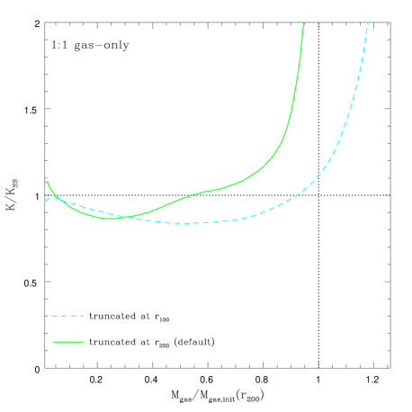
Figure 7: Testing the origin of excess entropy at large radii. Shown are the results of the 1:1 gas-only merger where the gaseous atmospheres have initially been truncated at $r_{200}$ (i.e., the default setup) and at $r_{100}$. Extending the gaseous atmospheres to larger radii results in a more accurate density determination near $r_{200}$ which, in turn, mitigates the over-efficient entropy production seen at large radii in the default run.

In Figure 7, we compare the final $K(M_{\rm gas})$ distributions for the merged systems (normalised to the self-similar result) in the default and extended runs. For the central 40% of gas mass, the $K(M_{\rm gas})$ distributions are similar. However, beyond this point differences become readily apparent. Interestingly, for the run where the initial gas profiles were extended to $r_{100}$, the final $K(M_{\rm gas})$ distribution remains close to the self-similar result all the way out to $M_{200}$. Beyond this point, a deviation from self-similarity is seen, as in the default run. However, since within $M_{200}$ (or, equivalently, $r_{200}$) the systems in the extended and default runs are initially identical, we must conclude that the deviation from self-similarity seen at large in Fig. 5 (and similar figures) is indeed artificial and its origin is linked to a poor (SPH) estimate of the true gas density near the edges of the idealised systems.

Fortunately, the central regions of the default run are not significantly affected by how we treat the edge and therefore it is this region that we focus on when comparing to self-similar expectations or our analytic models. In particular, when constructing physical analytic models that describe our simulations in §4, we restrict our focus to radii corresponding to $M_{\rm gas}/M_{\rm gas,tot}<0.8$.

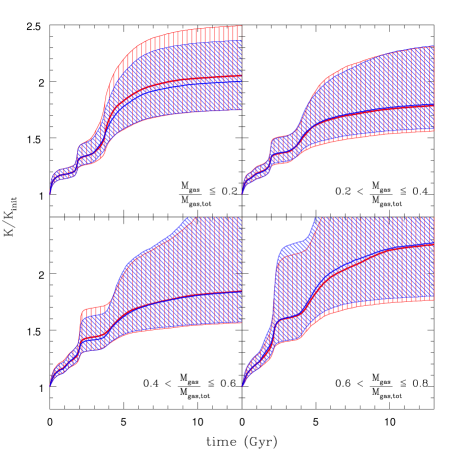
Figure 8: Entropy evolution in the head on 1:1 gas+DM merger. The red and blue lines/hatched regions represent the primary and secondary systems, respectively. The upper and lower bounds of the hatched regions represent the 75^th and 25^th percentiles, respectively, while the central (thick) lines represent the median. The panels show the evolution of the entropy of particles separated according to their initial position in the cumulative gas mass profile. Since the cumulative gas mass profile is a monotonic function of radius, the panels also separate the particles according to initial distance from the centre of their respective halos.

3.2 Gas + dark matter (gas+DM) simulations

3.2.1 Entropy evolution

In Figure 8 we plot the evolution of the entropy with time for the head on 1:1 gas+DM simulation. Several differences are apparent between the evolution in this figure and that of the 1:1 gas-only simulation plotted in Figure 2. For example, the gas+DM run shows evidence for a small amount of entropy production right from the start of the simulation, whereas the gas-only run does not (at least not within the central regions). This difference may be attributed to the different methods used for constructing the initial conditions. In an azimuthally averaged sense, both the gas-only and gas+DM runs have, for our purposes, nearly identical initial conditions. However, because the initial gas particle positions in the gas+DM run were assigned based on the positions of dark matter particles (see §2.1.2), small local inhomogeneities are initially present in these runs. As a result, the gas is not in perfect hydrostatic equilibrium and the systems undergo a slight re-adjustment when the simulation starts. Fortunately, the amount of entropy generated in this re-adjustment is small compared to the entropy produced in the merger shock heating and can be safely ignored. This is demonstrated below when we make an explicit comparison of the gas-only and gas+DM results.

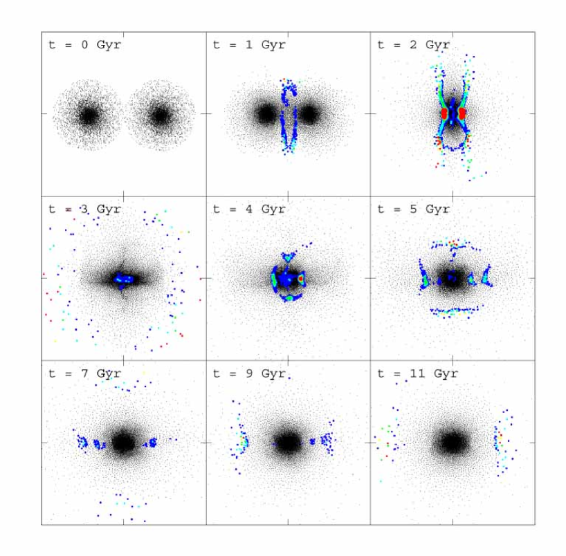
Figure 9: Fractional change in particle entropy as a function of time for the head on 1:1 gas+DM merger. Shown are particles in a slice through the centre of thickness 250 kpc (i.e., $|z|<125$ kpc). Particles are colour coded according to the fractional change in entropy since the last simulation output (0.1 Gyr ago). Black points are for a fractional change of less than 2%, blue are for a 2%-10% change, cyan are for a 10%-20% change, green are for a 20%-30% change, yellow are for a 30%-40% change, and red are for a $>$ 40% change. For clarity the surrounding pressure-confining medium is not displayed. Each panel is 10 Mpc on a side.

The most important changes between Figs. 2 and 8 relate to the properties of the second (proper) period of entropy generation. In particular, the second phase of heating, which was associated with a series of re-accretion shocks in the gas-only runs, begins earlier, rises more steeply, and contributes more to the final state of the system (particularly in the central regions) in the gas+DM run than in the gas-only run. What is the origin of this behaviour?

To help answer this question, we plot in Fig. 9 a series of snapshots colour coded according to the fractional change in entropy since the last simulation output (see Fig. 3 for the analogous plot for the gas-only run). The evolution is quite similar to that of the gas-only run early on. However, noticeable differences are present between the two at intermediate times ($t\sim 4-5$ Gyr). In particular, in the gas+DM run it is apparent that a second fast moving shock wave has been generated. This shock wave propagates outward in a nearly spherical fashion and resembles that of the first shock created when the cores collided. The origin of this second shock can be linked to the collisionless nature of the dark matter, which allows the dark matter cores to pass through one another, while the gas cores collide. Since the dark matter dominates the gas by mass, and the dark core is able to drag significant quantities of gas into the other hemisphere and away from the overall system’s centre of mass. As a result, some of the gas undergoes a second period of collapse, collides with gas infalling from the other hemisphere, and produces the shock. It is demonstrated later that the extra energy required for this second shock is derived from tapping the dark matter component (see, e.g., Fig. 21). Following this second shock, there is an extended period of re-accretion that proceeds in a similar fashion to that in the gas-only run. It is the combination of this second shock and the re-accretion phase that is responsible for the increased importance of the second major phase of entropy production in Fig. 8.

The head on 3:1 and 10:1 gas+DM mergers also show the same qualitative trends. But the head on case is special and, therefore, the final state of such collisions may not be representative of typical mergers in cosmological simulations. On the other hand, cosmological simulations suggest that groups and clusters acquire the bulk of their mass by substructure falling in along filaments. So the head on scenario will not be as far removed from the typical merger event as in the case of collisions between galaxies. However, it is still important to quantify the differences between the head on and non-zero impact parameter cases.

In Figures 10-15 we compare snapshots showing the spatial distributions of the primary and secondary particles and also the fractional change in entropy since the last simulation output for the all of the gas+DM merger simulations. We omit the panel showing the initial particle positions at $t=0$, since they are the same for the three different orbital cases (thus, the energy to be thermalised is the same for all three cases). In these figures, the centre of each panel corresponds to the overall centre of mass, with the secondary system initially approaching from the left and the primary from the right. In the non-zero impact parameter runs, the secondary’s initial motion is towards the upper right, while the primary is initially moving towards the lower left.

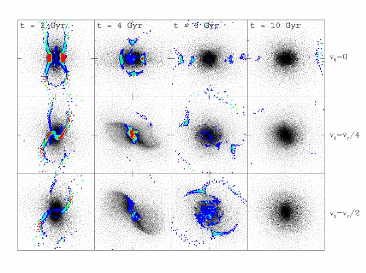
Figure 10: Fractional change in particle entropy as a function of time for the 1:1 gas+DM mergers. Top: Head on case. Middle: Small impact parameter case. Bottom: Large impact parameter case. Particle colour coding is the same as in Figure 9. Each panel is 6 Mpc on a side.

Figure 11: Spatial distributions of particles originally belonging to the primary (red) and secondary (blue) systems for the 1:1 gas+DM mergers. Top: Head on case. Middle: Small impact parameter case. Bottom: Large impact parameter case. For clarity, the secondary particles are plotted on top of the primary particles. Each panel is 6 Mpc on a side.

Figure 12: Fractional change in particle entropy as a function of time for the 3:1 gas+DM mergers. Top: Head on case. Middle: Small impact parameter case. Bottom: Large impact parameter case. Particle colour coding is the same as in Figure 9. Each panel is 6 Mpc on a side.

Figure 13: Spatial distributions of particles originally belonging to the primary (red) and secondary (blue) systems for the 3:1 gas+DM mergers. Top: Head on case. Middle: Small impact parameter case. Bottom: Large impact parameter case. For clarity, the secondary particles are plotted on top of the primary particles. Each panel is 6 Mpc on a side.

Figure 14: Fractional change in particle entropy as a function of time for the 10:1 gas+DM mergers. Top: Head on case. Middle: Small impact parameter case. Bottom: Large impact parameter case. Particle colour coding is the same as in Figure 9. Each panel is 6 Mpc on a side.

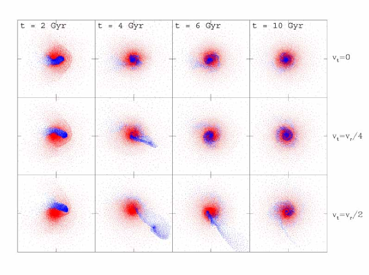
Figure 15: Spatial distributions of particles originally belonging to the primary (red) and secondary (blue) systems for the 10:1 gas+DM mergers. Top: Head on case. Middle: Small impact parameter case. Bottom: Large impact parameter case. For clarity, the secondary particles are plotted on top of the primary particles. Each panel is 6 Mpc on a side.

The general progressions of the 1:1 non-zero impact parameter cases, presented in Figs. 10 and 11, are as follows. In the small impact parameter case (where $v_{t}=v_{r}/4$ initially) the cores graze each other after $t\approx 2$ Gyr of infall. As a result, the cores are temporarily spared from significant shock heating. However, the systems are gravitationally bound and cannot avoid a major collision for long. In short order the cores cease moving apart and begin falling inward nearly radially, setting up an almost head on secondary collision (at $t\approx 4$ Gyr) that greatly heats the core gas. Additional small shocks are generated by the back and forth sloshing of the dark matter cores, but in general their contribution to the entropy production is minor. As in the cases examined above, an extended period of re-accretion then ensues. In this case, the bulk of the accretion first happens preferentially along and perpendicular to the axis of the secondary (near head on) collision. Qualitatively, the large impact parameter case proceeds much the same way. The main differences are as follows. The larger impact parameter means that the gas cores go virtually unheated during the first pericentric passage, as the cores of the two systems completely miss one another. The larger impact parameter also implies the amount of time spent between the first and second pericentric passages will be longer. Furthermore, the secondary collision is not directly head on in this case, meaning that some of the gas actually undergoes a third pericentric passage before settling. In both the small and large impact parameter cases, significant angular momentum is imparted to the gas and large, nearly circular, bulk motions remain present until the end of the simulations.

Figs. 12-15 are completely analogous plots for the 3:1 and 10:1 cases. In both head on collisions, the secondary essentially acts like a bullet, driving a large shock into the gas of the primary system and is able to easily penetrate all the way to the core of the primary. In fact, unlike the head on 1:1 case, the core of the secondary in the 3:1 and 10:1 cases is able to remain somewhat intact even after a collision with the core of the primary. As a result, there is actually a period where the cores pass through one another. However, the tidal forces exerted on the secondary’s core significantly stretch it along the collision axis. A second head on collision between the cores of the two systems then occurs. At the same time, the sloshing back and forth of the dark matter cores is generating small shocks. The small and large impact parameter 3:1 and 10:1 cases show evidence for even more complicated behaviour, with multiple collisions occurring and shock waves propagating in various directions simultaneously.

Figure 16: The resulting $K(M_{\rm gas})$ distributions for the 1:1 gas+DM mergers. Left: Comparison of the final entropy distributions for the primary (short-dashed red), secondary (long-dashed blue), and total (solid green) systems for the three different orbital cases. Right: Comparison of the final entropy distributions of the total systems in the gas+DM mergers for the head on (solid red), small impact parameter (short-dashed green), and large impact parameter (long-dashed blue) systems and the gas-only head on merger (dot-dashed magenta). The horizontal dotted line represents the self-similar scaling.

3.2.2 Final configurations

Given the wide variety of behaviours seen in Figs. 10-15, one might reasonably expect that the resulting gas properties of the various mergers to be significantly different from one another. But an analysis of the final entropy distributions indicates otherwise. Plotted in Figures 16a,b are the final $K(M_{\rm gas})$ distributions for the various 1:1 mergers. In Fig. 16a, it is demonstrated that the bulk of the gas in the primary, secondary, and total systems nearly maintain self-similarity. However, it is apparent that the small and large impact parameter cases show evidence for excess heating of the core gas relative to the head on case. This is illustrated most clearly in Fig. 16b, which compares the $K(M_{\rm gas})$ distributions for the total systems of the three different gas+DM simulations. This plot shows that the cases with non-zero impact parameter heat the core at the expense of the outer regions of the systems. However, it is remarkable that only the central $\sim$20% of the gas mass show significant deviations from the head on case given the large modifications to the initial orbital parameters. It is worth noting that non-radiative cosmological simulations also show evidence that the gas departs from a pure hydrostatic NFW profile in cores of systems (e.g., Frenk et al. 1999; Voit et al. 2005). So some deviation from self-similarity in our simulations might be expected.

Also plotted in Fig. 16b is the $K(M_{\rm gas})$ distribution for the 1:1 gas-only merger. Outside the central regions, it traces the distribution of the head on gas+DM simulation remarkably well. The two distributions begin to deviate from one another for $M_{\rm gas}/M_{\rm gas,tot}<0.4$ or so. The excess heating in the gas+DM can plausibly be attributed to energy exchange between the gas and the dark matter (see, e.g., Lin et al. 2006). In §4, we show that typically 5-10% of the dark matter’s energy is transferred to gas. This energy exchange occurs during the period when the dark matter cores of the primary and secondary are oscillating back and forth.

In Figures 17a,b we compare the final $K(M_{\rm gas})$ distributions for the various 3:1 mergers. Fig. 17a shows that the bulk of the gas for the total systems in all three orbit cases nearly obey self-similarity. As in the gas-only mergers discussed in §3.1, self-similarity is achieved by over-heating the primary and under-heating the secondary. Similar to the 1:1 gas+DM mergers discussed immediately above, the 3:1 mergers also show evidence for departures from self-similarity for the central 20% or so of the total gas mass. A comparison of the final distributions for the total systems in Fig. 17b illustrates this more clearly. Interestingly, even the head on 3:1 case shows evidence for strong central heating. In fact, the head on case appears to be even slightly more efficient at heating the core than the case characterised by a large impact parameter. (But we note that in the large impact parameter case there is still some residual heating occurring at the end of the simulation, so in the long run it may be the more efficient of the two.) A comparison of the entropy distributions of the head on gas+DM and gas-only mergers again highlights the fact that the two differ from each other only in the very central regions.

Finally, in Figures 18a,b we show the same set of plots for the 10:1 gas+DM mergers. The trends in these plots follow those discussed above for the 1:1 and 3:1 mergers. The only difference that we would mention is that the 10:1 cases exhibit a much lesser degree of central heating than the simulations discussed previously.

Figure 17: The resulting $K(M_{\rm gas})$ distributions for the 3:1 gas+DM mergers. Left: Comparison of the final entropy distributions for the primary (short-dashed red), secondary (long-dashed blue), and total (solid green) systems for the three different orbital cases. Right: Comparison of the final entropy distributions of the total systems in the gas+DM mergers for the head on (solid red), small impact parameter (short-dashed green), and large impact parameter (long-dashed blue) systems and the gas-only head on merger (dot-dashed magenta). The horizontal dotted line represents the self-similar scaling.

Figure 18: The resulting $K(M_{\rm gas})$ distributions for the 10:1 gas+DM mergers. Left: Comparison of the final entropy distributions for the primary (short-dashed red), secondary (long-dashed blue), and total (solid green) systems for the three different orbital cases. Right: Comparison of the final entropy distributions of the total systems in the gas+DM mergers for the head on (solid red), small impact parameter (short-dashed green), and large impact parameter (long-dashed blue) systems and the gas-only head on merger (dot-dashed magenta). The horizontal dotted line represents the self-similar scaling.

3.3 Summary of Simulation Results

In the next section we develop a physically-motivated analytic model that attempts to encapsulate the key physics of the merging process just described. However, before presenting this model we summarise the results of our simulations:

• Both the primary and secondary systems gain the bulk of their final entropy through two distinct episodes. The first episode is associated with a strong, quickly propagating shock wave that is generated approximately when the cores of the two systems collide. The second episode of heating occurs over an extended period of time. In the gas-only simulations, this second phase is driven entirely by a series of re-accretion shocks. In the gas+DM simulations, it is driven by a combination of re-accretion shocks and energy transfer from the dark matter to the gas, with the re-accretion shocks playing the dominant role.

• In all of our simulations, the contributions of the first and second episodes of entropy production to the final distribution are comparable.

• We find that the bulk of the gas in our simulations matches the self-similar result to within 10%. Deviations from self-similarity are seen at large radii in both the gas-only and gas+DM simulations. This is almost certainly due to a truncation effect in our idealised setup (see §3.1.3). Deviations from self-similarity are also seen at small radii in the gas+DM simulations (which are real) and are at least partially due to energy exchange between the gas and dark matter. Some deviation might be expected at small radii, as the gas in systems formed in non-radiative cosmological simulations also show departures there from a pure hydrostatic NFW distribution.

• With the obvious exception of the symmetric 1:1 case, self-similarity of the final merged system is achieved by over-heating the gas in the primary while under-heating the gas in the secondary. This implies that some of the infall energy initially associated with the secondary has gone into heating the primary.

Our simulations therefore differ markedly from the standard spherical smooth accretion model where the ICM is built up one shell at a time from the inside out and where each shell is shocked a single time as it enters the virial radius. It seems remarkable that these two very physically different scenarios yield structural properties that are as similar as they are. However, as discussed in detail by Voit et al. (2003), the spherical accretion model fails to match the results of cosmological simulations when it is modified to account for more realistic “lumpy” accretion. The reason for this failure is that increasing the density but keeping the total energy to be thermalised fixed results in decreased entropy production in the shock. However, our simulations show that significant shock heating does not occur until core collision. As a result, there is significantly more infall energy available for thermalisation. To a large extent, this boost offsets the otherwise reduced level of entropy owing to the increased density of infalling gas in the lumpy model relative to the smooth accretion model.

4 Discussion: Understanding the Results

4.1 A Simple Single-Shock Model

We have demonstrated that our idealised merger simulations approximately preserve self-similarity, as seen in non-radiative cosmological simulations. As a result, we are now in a position to try to develop a physical analytic model for the entropy evolution of the primary and secondary systems in our idealised simulations. Taking our cue from the study of Voit et al. (2003), we consider a simple model whereby gas with some initial density $\rho_{1}$ and entropy $K_{1}$ is moving with a velocity $v_{\rm in}$ in the system’s centre-of-mass frame. If this velocity is supersonic it will generate a shock front. Assuming that the post-shock gas is at rest in the centre-of-mass frame (i.e., that all of the energy associated with $v_{\rm in}$ is thermalised), then the shock propagates with a velocity $v_{\rm shock}$ into the gas in the centre-of-mass frame. In the rest-frame of the shock, the gas therefore has a velocity $v_{1}=v_{\rm in}+v_{\rm shock}$, and the post-shock gas has a velocity $v_{2}=v_{\rm shock}$. The pre-shock (upstream) conditions are related to the post-shock (downstream) conditions via the well-known Rankine-Hugoniot jump conditions (e.g., Shu 1992):

$$\frac{\rho_{2}}{\rho_{1}}=\frac{v1}{v2}=\frac{(\gamma+1){\cal M}_{1}^{2}}{(\gamma-1){\cal M}_{1}^{2}+2},$$ (8)

$$\frac{P_{2}}{P_{1}}=1+\frac{2\gamma({\cal M}_{1}^{2}-1)}{\gamma+1}$$ (9)

$$\frac{T_{2}}{T_{1}}=\frac{[1+\gamma(2{\cal M}_{1}^{2}-1)][2+(\gamma-1){\cal M}_{1}^{2}]}{(\gamma+1)^{2}{\cal M}_{1}^{2}}$$ (10)

where ${\cal M}_{1}\equiv v_{1}/c_{s}$ is the Mach number. Equations (8) and (9) can be used to yield the jump condition relating pre-shock and post-shock entropy:

$$\frac{K_{2}}{K_{1}}=\biggl{[}\frac{5{\cal M}_{1}^{2}-1}{4}\biggr{]}\biggl{[}\frac{4{\cal M}_{1}^{2}}{{\cal M}_{1}^{2}+3}\biggr{]}^{-5/3}$$ (11)

where we have used $\gamma=5/3$. Therefore, one can calculate the final entropy distribution if the Mach number of the shock is known. Unfortunately, it is non-trivial to measure the Mach number of a shock directly from the simulations. Shock heating is implemented in SPH simulations via an artificial viscosity term which significantly broadens the shocks both spatially and temporally. This prevents one from easily applying equations (8)-(11) to individual SPH particles (see Pfrommer et al. 2006). Another difficulty is that the Mach number is expressed in terms of pre-shock velocity in the rest-frame of the shock. So application of these equations to individual particles would require one to carefully track the evolution of the shock itself during the simulation. To avoid these difficulties, we use equation (8) to instead express the Mach number in terms of the difference between the pre-shock and post-shock velocities:

$$v_{1}-v_{2}=v_{\rm in}=\frac{3}{4}\biggl{[}1-\frac{1}{{\cal M}^{2}_{1}}\biggr{]}v_{1}$$ (12)

Rearranging and replacing $v_{1}$ by ${\cal M}_{1}c_{s}$, we obtain

$$v_{\rm in}=\frac{3}{4}\biggl{[}\frac{{\cal M}_{1}^{2}-1}{{\cal M}_{1}}\biggr{]}c_{s}=\frac{3}{4}\biggl{[}\frac{{\cal M}_{1}^{2}-1}{{\cal M}_{1}}\biggr{]}\biggl{[}\frac{5}{3}K_{1}\rho_{1}^{2/3}\biggr{]}^{1/2}$$ (13)

Figure 19: Comparison of the final entropy distribution of the primary in the 1:1 (left) and 3:1 and 10:1 (right) gas-only simulation with our simple analytic shock heating model. The thick red curve represents the simulation result. The dashed curves represent the simple analytic model (equations 11 & 13) for choices of $v_{in}/v_{c,p}(r_{200})$ ranging from $0.75-2.00$ in steps of $0.25$ (bottom to top).

Therefore, given the initial entropy and density distributions of the gas and the velocity of the gas in the centre-of-mass frame, it is possible to solve the quadratic equation (13) for the Mach number of each particle. Deriving the final entropy distribution is then simply a matter of plugging these Mach numbers into equation (11). Of course in our idealised merger simulations we know precisely what the initial entropy and density profiles of the systems are, but what velocity do we pick for $v_{\rm in}$? Various possibilities exist, but $v_{\rm in}$ should not exceed the relative velocity of the cores as they are about to collide (i.e., when the gravitational energy between the two systems has been maximally converted to infall energy). In fact, the velocity will have to be quite a bit lower than this since, for example, in the 1:1 case using the maximum relative velocity for the gas in both systems would require twice as much energy as there is available to be thermalised. Unfortunately, given the complicated nature of the simulations, the correct value of $v_{\rm in}$ could fall any where between zero and this upper bound. Previous analytic studies (e.g., Voit et al. 2003) adopted the infall velocity at the virial radius. However, it is evident from §3 that significant shock heating does not occur in our simulations until the cores of the two systems nearly collide. As a result, the infall velocity will be much larger than assumed in those analytic studies. Furthermore, it is also clear that energy is being exchanged between the primary and the secondary systems (for example, even in the 10:1 case the secondary is capable of driving a shock that significantly heats virtually all of the gas in the primary). This makes it even more difficult to assess a priori what is the appropriate value of $v_{\rm in}$ to assign for the primary and secondary systems.

We sidestep this problem by inverting the question: i.e., given the initial entropy and density profiles, what velocity is required to explain the final entropy distribution? To answer this question we simply try a range of different values for $v_{\rm in}$ and assess which gives the best match to the final entropy distribution. This velocity can be cast in terms of a requirement for the total amount of energy that must have been thermalised in order to explain the final entropy distribution. In §4.2, we examine whether or not there is enough bulk energy available to explain our findings.

Although the simulated systems undergo two periods of entropy production, we start by trying to use the single-shock model outlined above to explain the observations. In principle this model, which just uses continuity and conservation equations to link upstream and downstream conditions, can effectively describe physical situations that are more complex than a single shock. Therefore it is the natural starting point for our investigation.

We start by first examining the gas-only simulations, which make a useful benchmark for the more realistic gas+DM runs. In Figures 19a and 19b, the final entropy distributions of the primary and secondary systems in the 1:1, 3:1, and 10:1 gas-only mergers are compared with the simple analytic shock heating model proposed above. For the analytic model, the upstream values of the entropy and density are taken from the initial conditions of the simulations (see §2). We try several different values of $v_{\rm in}$ for both the primary and secondary systems, each corresponding to a unique prediction for the final entropy distribution of both systems. All curves plotted in Figs. 19a & 19b have been normalised to the self-similar expectation. In the discussion that follows, we exclude the high entropy tail at large values of $M_{\rm gas}/M_{\rm gas,tot}$ from consideration. The §3.1.3 shows that this tail results from the truncation of our idealised halos.

Figs. 19a & 19b show that a centre-of-mass velocity ranging approximately from $0.9<v_{\rm in}/v_{c,p}(r_{200})<1.25$ is required to explain the final entropy distributions of the primary systems in the three runs. The secondary systems require slightly lower velocities ranging from $0.75<v_{\rm in}/v_{c,p}(r_{200})<1.25$. For both the primary and secondary systems there is a trend with the mass ratio of the merger, in the sense that the higher the mass ratio the lower the required velocity is to explain their final entropy distributions. It is worth noting, however, that no single choice of $v_{\rm in}$ can explain the entire $K(M_{\rm gas})$ profiles for the primary and secondary systems. In particular, if the analytic model is normalised to explain the intermediate regions of the entropy profiles (say $0.3<M_{\rm gas}/M_{\rm gas,tot}<0.6$), it systematically under-predicts the level of the lowest entropy gas ($M_{\rm gas}/M_{\rm gas,tot}<0.2$) compared to the simulations. Nevertheless, the bulk of the gas in the primary and secondary systems can be adequately modelled by a fairly small range of velocities.

Figure 20: Comparison of the final entropy distribution of the primary in the 1:1 (left) and 3:1 and 10:1 (right) gas+DM simulation with our simple analytic shock heating model. The thick red curve represents the simulation result. The dashed curves represent the simple analytic model (equations 11 & 13) for choices of $v_{in}/v_{c,p}(r_{200})$ ranging from $0.75-2.00$ in steps of $0.25$ (bottom to top).

An identical set of plots is presented in Figures 20a,b for the gas+DM simulations. Note that significantly higher velocities are required to explain the final entropy distributions of the primary and secondary systems in the gas+DM simulations. In particular, the primary systems typically require velocities ranging from $1.35<v_{\rm in}/v_{c,p}(r_{200})<1.80$, while the secondaries typically require $1.00<v_{\rm in}/v_{c,p}(r_{200})<1.80$ (see Table 2). Even though the systems in the gas+DM simulations require significantly higher velocities than those in the gas-only simulations this does not necessarily imply that the energetic requirements of gas+DM mergers exceed those of the gas-only mergers. It should be kept in mind that for a system of mass $M_{200}$ there is simply much more gas that requires heating in the gas-only simulations (the baryon to total mass ratio of the gas-only simulations is $\approx$7 times larger than the gas+DM simulations). Below we compare the energy required by the simple shock heating model to match level of entropy production seen in the idealised simulations with our best estimates of the amount of energy available.

4.2 Energy Considerations

If we assume that the simple shock heating model provides a reasonable description of what is taking place in the simulations, the velocity $v_{\rm in}$ can be used to estimate the total amount of energy that was thermalised in producing the final entropy distributions. Conveniently, $v_{\rm in}$ is defined such that the post-shock gas is at rest in the centre-of-mass frame, so the total thermalised energy is just:

$$E_{\rm T,tot}=E_{\rm T,p}+E_{\rm T,s}=\frac{1}{2}M_{\rm gas,p}v_{\rm in,p}^{2}+\frac{1}{2}M_{\rm gas,s}v_{\rm in,s}^{2}$$ (14)

Typically, this results in values ranging from approximately $2-6\times 10^{64}$ ergs for the gas-only mergers and $0.5-2\times 10^{64}$ ergs for the gas+DM mergers. So even though the gas+DM mergers require higher velocities to preserve self-similarity, their energy requirements are lower than those of the gas-only simulations. As mentioned above, this is simply because there is more gas that requires heating in the gas-only simulations.

Interestingly, even though the energetic requirements are different between the two types of simulations, the way the energy is distributed does not appear to be. In particular, in both types of simulations the thermalisation of the primary’s gas dominates the thermalisation energy budget with 50%, $\approx$80%, and $\approx$95% of the total energy in the 1:1, 3:1, and 10:1 mergers, respectively (see Table 2). The following analytic relationship yields a remarkably good fit to our simulated mergers (including those involving mass ratios not presented in this paper):

$$\frac{E_{\rm T,p}}{E_{\rm T,s}}\approx\biggl{(}\frac{M_{\rm p}}{M_{\rm s}}\biggr{)}^{5/4}$$ (15)

Interestingly, this is quite close to the case where the primary and secondary thermalise each other’s infall energy, i.e., $E_{\rm T,p}/E_{\rm T,s}=M_{p}/M_{s}$. We also note that this type of scaling is naturally achieved if each gas particle thermalises the same fraction of the total available energy. This interesting result deserves further investigation, which we take up in the next paper of this series.

Table 2: Single-Shock Model Velocity/Energy Requirements

$M_{p}/M_{s}$	Sim. type	$v_{\rm in,p}$	$v_{\rm in,s}$	$E_{T,p}/E_{T,tot}$
		$[v_{c,p}(r_{200})]$	$[v_{c,p}(r_{200})]$
1:1	gas-only	1.25	1.25	0.50
3:1	gas-only	1.25	1.00	0.82
10:1	gas-only	0.9	0.75	0.94
1:1	gas+DM	1.8	1.8	0.50
3:1	gas+DM	1.65	1.35	0.82
10:1	gas+DM	1.35	1.00	0.95

An important consistency check of the simple shock heating model is to test whether or not there is enough energy available to meet the requirements of the model. Having too much energy available isn’t necessarily a problem, since there are numerous ways the available energy could be tapped (e.g., some could go into bulk kinetic circular motions of the gas or into the dark matter in the case of the gas+DM simulations). However, if there isn’t enough energy available, the only possibility is that the model is incorrect or, at best, incomplete.

With this in mind, we calculate the energy available to be thermalised in our idealised mergers. We do so via two different methods, with both yielding similar results. The first method, which we refer to as the “simulation method”, takes advantage of the excellent energy conservation of the GADGET-2 simulations. The total energy of the gas is

$$E_{\rm tot,gas}(t)=E_{\rm K_{\rm gas}}(t)+E_{\rm U_{\rm gas}}(t)+E_{\rm I_{\rm gas}}(t)$$ (16)

where $E_{\rm K_{\rm gas}}(t)$, $E_{\rm U_{\rm gas}}(t)$, and $E_{\rm I_{\rm gas}}(t)$ are the kinetic, potential, and internal (thermal) energies of the gas at time $t$. $E_{\rm tot,gas}(t)$ is conserved in the gas-only simulations to better than 1%. Therefore, we can write

$$E_{\rm K_{\rm gas}}(t)+E_{\rm U_{\rm gas}}(t)+E_{\rm I_{\rm gas}}(t)=E_{\rm K_{\rm gas}0}+E_{\rm U_{\rm gas}0}+E_{\rm I_{\rm gas},0}$$ (17)

where $E_{\rm K_{\rm gas},0}$, $E_{\rm U_{\rm gas},0}$, and $E_{\rm I_{\rm gas},0}$ are the values of the three different energies at the start of the simulation. The total energy that is available to be thermalised at time $t$ is just the initial (centre-of-mass) kinetic energy plus the change in the gravitational potential energy:

$$E_{\rm T,tot}(t)=E_{\rm K_{\rm gas},0}-[E_{\rm U_{\rm gas}}(t)-E_{\rm U_{\rm gas},0}]$$ (18)

which is relatively trivial to measure in the simulations. This energy estimate can be compared directly with the simple shock heating model estimate in equation (14).

However, the above treatment is strictly only valid for the gas-only simulations. In the gas+DM simulations, energy can be exchanged between the gas and the dark matter. But we can take advantage of the fact that the summation of the total energy of the gas and the total energy of the dark matter is conserved in these simulations. Thus, for the gas+DM simulations we modify equation (18) to read

$$E_{\rm T,tot}=E_{\rm K_{\rm gas},0}+[E_{\rm U_{\rm gas}}(t)-E_{\rm U_{\rm gas},0}]-E_{\rm DM\leftrightarrow gas}(t)$$ (19)

where

$$E_{\rm DM\leftrightarrow gas}(t) \equiv [E_{\rm K_{DM}}(t)+E_{\rm U_{DM}}(t)]$$

$$-[E_{\rm K_{DM},0}+E_{\rm U_{DM},0}]$$

is the energy exchanged between the gas and dark matter.

In principle, this energy exchange can go either way, but in general we find that the dark matter loses energy to the gas. In Figure 21, we plot the evolution of the energy associated with the dark matter in the gas+DM simulations (see caption). By the end of the simulations, we find that the dark matter in the 1:1, 3:1, and 10:1 mergers has lost approximately 7-10%, 7-9%, and 2-3%, respectively, of its energy to the gas. Interestingly, this estimate doesn’t depend much on the adopted orbital parameters, nor the mass resolution of the simulation. We will return to this issue of energy exchange below.

The second method that we use to calculate the energy available to be thermalised, which we refer to as the “analytic method”, is as follows. If we assume that the primary and secondary remain completely intact from their initial setup until the point when the centres of the two systems coincide, it is straightforward to calculate the total energy to be thermalised. Neglecting the thermal energy of the systems (which remains fixed with time by construction), the total energy of the gas in the centre-of-mass frame is

$$E_{\rm tot,gas}=\frac{1}{2}\mu v_{rel}^{2}+U_{\rm gas,ps}(r_{\rm ps})$$ (21)

where $\mu\equiv M_{\rm gas,p}M_{\rm gas,s}/(M_{\rm gas,p}+M_{\rm gas,s})$ is the reduced mass, $v_{rel}$ is the initial relative velocity between the primary and secondary systems, $r_{\rm ps}$ is the separation of their centres, and $U_{\rm gas,ps}$ is the gravitational potential energy. Assuming that the primary and secondary systems are rigid and ignoring the potential energy of the systems due to themselves (which, again, does not change by construction), the potential energy of interaction between the two systems is

$$U_{\rm gas,ps}(r_{\rm ps}) = \frac{1}{2}\int\phi_{\rm p}dM_{\rm gas,s}+\frac{1}{2}\int\phi_{\rm s}dM_{\rm gas,p}$$ (22)

$$= \frac{1}{2}\int\rho_{\rm gas,s}\phi_{\rm p}d^{3}V+\frac{1}{2}\int\rho_{\rm gas,p}\phi_{\rm s}d^{3}V$$

where $\phi$, the gravitational potential, is defined as

$$\phi(x)\equiv-G\int\frac{\rho(x^{\prime})}{|x^{\prime}-x|}d^{3}V^{\prime}$$ (23)

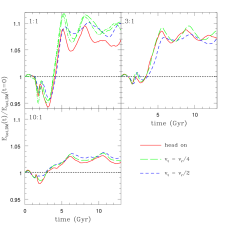
Figure 21: Evolution of the total energy of the dark matter in the gas+DM simulations. The energy has been normalised to its initial value. Since the systems are bound the total energies are negative. Thus, a value of $E_{\rm tot,DM}(t)/E_{\rm tot,DM}(t=0)$ greater than unity implies that energy has been lost to the gas, while a value less than unity means energy has been extracted from the gas. The green dot-dashed curve in the 1:1 panel is for the highest resolution simulation in the mass resolution study in the Appendix.

Approximating the systems as point masses initially, when there is little or no overlap between them, the potential energy of the gas is just

Figure 22: Comparison of the shock heating model’s energy requirements with the maximum energy available to be thermalised in the gas-only (left) and gas+DM (right) simulations. In the panels on the right, the short-dashed red curves represent the results of the simulation method shifted up by $E_{\rm tot,DM}(t=13{\rm Gyr})-E_{\rm tot,DM}(t=0)$, i.e., by the total amount of energy lost by the dark mark to gas by the end of the simulation. For comparison, the dot-dashed blue lines represent the gas-only simulations, which have been renormalised by multiplying the energy by the baryon fraction of the gas+DM systems.

$$U_{\rm gas,ps}(r_{\rm ps}=d_{0}) = -\frac{1}{2}\frac{G}{d_{0}}\biggl{[}M_{\rm p}M_{\rm gas,s}+M_{\rm p,gas}M_{\rm s}\biggr{]}$$

$$= -\frac{Gf_{b}M_{p}M_{s}}{d_{0}}$$

where the second line is true only if both the primary and secondary systems have the same baryon fraction.

Therefore, the total energy of the gas is

$$E_{\rm tot,gas}=\frac{1}{2}\mu[v_{\rm c,p}(r_{200})]^{2}-\frac{Gf_{b}M_{p}M_{s}}{d_{0}}$$ (25)

The maximum energy available to be thermalised occurs when the centres of the primary and secondary coincide. We can therefore calculate the maximum energy available to be thermalised by subtracting the potential energy when the systems coincide (calculated by evaluating equation 22) from the total energy given in equation (25).

In Figures 22a,b, we compare the simple shock heating model’s energy requirements (see Table 2) with the energy available to be thermalised as estimated by both the simulation and analytic methods described above. We focus first on the gas-only results plotted in Fig. 22a. The solid curves represent the amount of energy available to be thermalised as estimated with the simulation method. The peak of the curves are reached at $t\approx 1.5$-$1.8$ Gyr, i.e., just slightly before the cores of the primary and secondary collide. The amplitude of the peak is within a few tens of percent of the maximum energy estimated via the analytic method (dotted line). This agreement indicates that our estimate of the maximum energy available for thermalisation is robust and also demonstrates that one can estimate this energy reasonably well using simple analytic modelling. A comparison to the dashed line, which represents the energy requirement of the simple shock heating model described in §4.1, yields interesting results. Apparently, the 1:1 gas-only merger has sufficient energy available to accommodate the shock heating model’s requirements. So the simple model provides a viable explanation for this collision. For the 3:1 gas-only merger there is a very small deficit of energy. However, in the case of the 10:1 gas-only merger, both the simulation method and analytic method estimates of the maximum amount of energy there is to be thermalised fall short of the required amount by roughly a factor of two.

Moving on to the gas+DM simulations in Fig. 22b, we find that there is insufficient energy available in any of the simulations to accommodate the requirements of the simple shock heating model (although the 1:1 is close). This is the case even when we account for the energy exchange between the gas and the dark matter. Thus, even though both the gas-only and gas+DM simulations preserve self-similarity, they do not give a consistent answer when compared to the simple analytic model. However, there are some similarities between the two in terms of their comparison with the analytic model. For example, both show a similar trend with mass ratio, in the sense that agreement gets worse for higher mass ratios. Furthermore, the energy shortfall is less than about a factor of $3$ for all of the simulations we have performed. Thus, while the simple analytic model fails to explain the results, it does not fail by a huge margin. This motivates us to consider modifications of the model.

4.3 A Double-Shock Model

In §3 we found that there are actually two major periods of entropy production experienced by the primary and secondary systems in our merger simulations. We now seek to modify the simple shock heating model presented in §4.1 to account for this behaviour. The relevant question is, for a fixed amount of energy to be thermalised, is a double-shock model capable of generating more entropy than a single-shock model? In the case where the post-shock conditions, as dictated by the jump conditions, simply become the pre-shock conditions for the second shock, we find that the answer is ‘no’. In general, we find that as one increases the number of shocks over which the energy is to be thermalised, the resulting final entropy decreases.

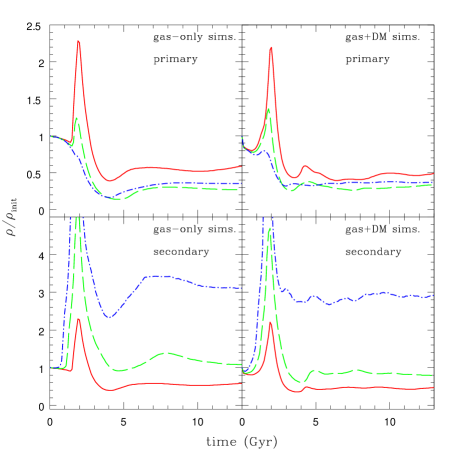
Figure 23: Evolution of the median density for particles that were located within the spherical shell $0.25\leq M_{\rm gas}/M_{\rm gas,tot}\leq 0.75$ initially. The solid red, dashed green, and dot-dashed blue curves represent the 1:1, 3:1, and 10:1 mergers, respectively. For the gas+DM simulations only the head on results are plotted. Note for the primary systems that the density drops below its initial (pre-merger) value between the end of the first shock and the onset of the second shock at $t\sim 4$ Gyr. For the secondary systems the density increases (except for the 1:1 case), as expected. However, only a small fraction of the total energy is thermalised in the secondary.

However, it quickly becomes apparent from an examination of the simulations that the properties of the gas evolve significantly between the end of the first shock and the onset of the second. In particular, there is a period of adiabatic expansion between the two shocks which likely arises as a result of the fact that not all the kinetic energy was thermalised in the first shock. The net result is that the typical density of the gas is significantly reduced between the shocks and can even drop below its pre-merger value (see Fig. 23). Furthermore, the drop is largest for the highest mass ratio mergers, precisely where we find the largest energy deficits between the simulations and the single-shock model. Dropping the density between the shocks will have the effect of increasing the amount of entropy generated in the second shock relative to the case where there is no adiabatic expansion between the shocks. More importantly, is the decrease in density between shocks large enough to generate more entropy than the single-shock model?

To answer this question, we have compared the single- and double-shock models head to head for an idealised parcel of gas with an initial density $\rho_{\rm init}$ and an initial entropy $K_{\rm init}$. In particular, in Fig. 24 we plot three sets of curves representing three different comparisons, each characterised by a different total amount of energy to be thermalised. The total energies have been chosen such that, in the single-shock model, the (shock frame) Mach numbers are 1.5, 2.5, and 3.5 (bottom to top). For the single-shock model, the Mach number is all that is required to predict the ratio of final to initial entropy (see equation 11). The three horizontal dotted lines in Fig. 24 represent the predictions of the single-shock model.

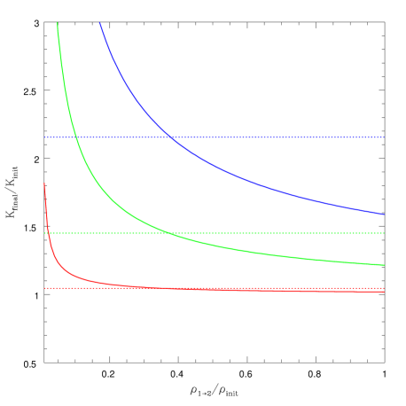
Figure 24: A comparison of the entropy generated by the single- and double-shock heating models. Horizontal dotted lines show the predictions of the single-shock heating model for (shock frame) Mach numbers of 1.5, 2.5., and 3.5 (bottom to top). The solid curves show the predictions of the double-shock model as a function of the density between the two shocks. Note that if the density drops below $\approx 40$% of its pre-merger value then the double-shock model generates more entropy than the single-shock model for a fixed amount of energy to be thermalised.

Figure 25: Final entropy predicted by the double-shock model as a function of the density $\rho_{1\rightarrow 2}$ between the two shocks for the gas-only (left) and gas+DM (right) simulations. The solid red, dashed green, and dot-dashed blue curves represent the 1:1, 3:1, and 10:1 mergers, respectively. The entropy has been normalised to the expected self-similar result, while the density has been normalised to its initial pre-merger value. The vertical dotted lines show the minimum density estimated from Fig. 23 at $t\approx 4$ Gyr.

For the double-shock model, we use the entropy and density evolution plots of the simulations as guides. Examination of the evolution of the entropy of our mergers (e.g., see Figs. 2, 4, and 8) indicates that the first and second shocks contribute comparable amounts of entropy to the final state. To first order, therefore, we surmise that the first and second shocks thermalise comparable amounts of energy (i.e., for the purposes of this toy model, we assume each shock thermalises half of the total energy.) Between the first and second shocks, there is a period of adiabatic expansion during which the density drops to some value $\rho_{1\rightarrow 2}$. Using the new density and entropy, we can solve for thermal energy of the gas (or, equivalently the sound speed). The ratio of the thermal energy to the remaining energy to be thermalised (i.e., half the initial energy) sets the Mach number of the second shock which, in turn, allows us to compute the final entropy.

In Fig. 24, the solid curves show the predicted trend between final entropy and density between the two shocks for double-shock model. A comparison between the single- and double-shock models demonstrates that if the density drops below about 40% of its initial pre-merger value then the double-shock model does indeed generate more entropy than the single-shock model. This is quite promising since Fig. 23 demonstrates that the primary systems, which dominate the thermalisation budget, have their densities reduced to at least this level (and lower for the 3:1 and 10:1 cases).

Given these results, we test the model further by tailoring the total energy to be thermalised (and, therefore, the Mach numbers) to match our merger simulations more closely. In particular, we assume the total energy is taken to be the peak of the solid curves plotted in Figs. 22a,b corresponding to the “simulation method” estimate. For simplicity, we further assume that each gas particle thermalises the same amount of energy. So, for example, the primary system thermalises $M_{p}/[M_{p}+M_{s}]$ times the total energy. As above, the Mach numbers are set by computing the ratios of thermal energy to energy to be thermalised for the first and second shocks.

In Figures 25a,b we plot the final entropy predicted by the double-shock model for the primary systems in our simulations. The entropy has been scaled to the self-similar result while $\rho_{1\rightarrow 2}$, the density between the two shocks, has been scaled to the initial pre-merger density. We use the vertical dotted lines, which are meant to represent the density minimum between the shocks seen in Fig. 23 (at $t\approx 4$ Gyr), to select the appropriate predicted entropy.

A comparison of the predicted entropy in Figs. 25a,b with that of the primary in our simulations in Figs. 5-6 (gas-only) and Figs. 16a, 17a, and 18a (gas+DM) demonstrates that in all cases, including the 10:1 mergers, the double-shock model can reproduce the simulation results to within 10%. Furthermore, we have found that this result is not very sensitive to the way in which we’ve distributed the energy over the two shocks. For example, we obtain very similar results if the second shock thermalises anywhere between 20-80% of the total energy, as opposed to half.

The double-shock heating model therefore appears to provide a simple framework for understanding the typical level of entropy generated in our mergers. In §5.3, we present a point by point algorithm that the reader can use to apply the double-shock model.

5 Conclusions

We have presented a series of simulations aimed at exploring the generation of entropy during cluster mergers. The results show that the entropy generated is remarkably robust. We show that the generation of entropy is largely independent of the impact parameter of the collision, and that similar results are obtained for simulations only involving gas and for mergers of systems that contain a cosmological mixture of gas and dark matter. The resulting entropy profiles also depend little on the resolution of the simulation, once more than $\sim 10^{4}$ particles are placed in each halo. These results hint that a general principle is at work, and that the generation of entropy can be understood as a general process that converts the gravitational potential energy released during the collapse of the system into the thermal energy of the ICM. Based on this reasoning, it should be possible to develop a simple model for the evolution of the entropy distribution as clusters grow in mass through mergers by examining the potential energy released in the collapse and the efficiency with which this is converted into thermal energy.

5.1 Equal mass mergers

We explore mergers of systems with a variety of mass ratios. In each case, we find that the entropy generated is approximately sufficient to place the final system on the same entropy scaling relation that was used to generate the original system. During equal mass mergers symmetry ensures that both systems are heated to the same degree. For the bulk of the gas, the powerlaw slope of the resulting entropy profile changes little compared to the original (see, e.g., Fig. 5a) and the degree of heating raises the normalisation of the entropy profile by $\approx 2^{2/3}$. As a result the final entropy distribution is scaled so that the final system is a self-similar copy of the original.

The exact process by which this entropy is generated is far from simple. The two clusters are in contact with each other at the start of the simulation, however, their infall velocity is not sufficiently high compared to the sound speed to generate a strong shock. The system becomes highly compact along the infalling axis with compressed material tending to flow out along the orthogonal plane. A strong shock is not generated until the cores of the two systems are superposed. At this point, a strong shock is generated, propagating rapidly out from the central regions. However, not all of the available infall energy is thermalised in this first shock. Some of it remains in kinetic form and succeeds in driving a period of adiabatic expansion. Eventually, however, the remaining energy is thermalised in a series of shocks as material is re-accreted by the merger remnant.

The generation of entropy thus shows two distinct peaks. The first corresponds to the strong shock generated as the cores collide, the second corresponding to the re-accretion of material that tried initially to escape from the system.

The delay to the initial shock in this system plays an important role in determining the entropy generated. Because the system collapses prior to the first shock, considerably greater binding energy is available to be thermalised. Superposing the initial mass distributions provides a good estimate of the available binding energy, and modelling this energy as being thermalised in a single strong shock provides a reasonable approximation to the entropy generated in the equal mass mergers.

5.2 Unequal mass mergers

For mergers between unequal mass halos, the generation of entropy is distributed unequally. Visually, we see that the smaller component remains essentially intact as it plunges into the centre of the main system (see, e.g., Figs. 13 and 15). We find that, although the kinetic energy of the collapsing system is primarily localised in the smaller mass system, this energy is largely thermalised in the more massive progenitor. As a result, the heating of the more massive progenitor exceeds what is predicted by the self-similar scaling relation

$$K\propto M^{2/3},$$

while the heating of the less massive component falls short of that needed for self-similarity. Despite this, the over- and under-heating of the components combine is such a way that the final system comes close to following the self-similar relation. We provide an analytic fit to the ratio of the energy dissipated in the two components in equation (15). This is close to assuming that the energy is exchanged between the primary and secondary components.

Thus we find that the mergers tend to produce scaled up copies of the original systems. This is good news since we started with systems having properties close to those of observed clusters, and we chose cosmologically likely values for the infall velocities. Our simulations show that the normalisation of this entropy profile is not a coincidence. Given the infall velocity distribution expected in a CDM universe this profile is a stable configuration.

As with the 1:1 merger case, we can estimate the energy that is available to be thermalised by tracking the evolution of the potential energy. This energy significantly exceeds the initial kinetic energy of initial system, showing that the long survival time of the secondary is responsible for much of the entropy generation. However, we find that a single shock model for the thermalisation of this energy under-predicts the entropy generated, particularly in the case of the 10:1 mass ratio. In order to match the entropy generation we find that it is necessary to model the two shock process that is seen in the simulations. A key ingredient of the entropy generation is the drop in the gas density as the system responds to the first shock. As the remaining binding energy is thermalised in this more diffuse medium, the entropy generation is more efficient.

5.3 An algorithm for computing shock heating

A good way to summarise the findings of this paper is to sketch out an algorithm for computing the entropy generated during the merger. Future papers will present the results from implementing this within cosmological merger trees. We summarise the algorithm as follows.

1.) Calculate the energy available for thermalisation. Cosmological simulations suggest that the secondary (less massive) system crosses the virial radius of the primary system with a total (relative) velocity of approximately the circular velocity of the primary system at that radius. The total energy is therefore given by equation (25). (Note, a similar energy estimate can be derived by calculating the potential energy between the systems at turnaround, when the relative kinetic energy is zero.) The energy available for thermalisation can then be obtained by subtracting from this the potential energy between the systems when their centres coincide (see §4.2).

2.) Distribute this energy in appropriate proportions to the primary and secondary systems. Our simulations indicate that the bulk of the energy is thermalised in the more massive primary system. Equation (15) provides a fit to how the energy should be divided up as a function of mass ratio.

3.) If the merger is 1:1 (or very nearly so), calculation of the post-shock properties is now straightforward. The energy estimated above can be converted into an estimate for the (centre-of-mass) velocity, $v_{in}$, for both systems. This, in turn, may be converted into an estimate of the (shock frame) Mach number (see equation 13). Calculation of the post-shock properties is then simply a matter of evaluating the Rankine-Hugoniot jump conditions (equations 8-11).

4.) If the mass ratio is different from unity, distribute the energy over two shocks. Our simulations suggest that the two shocks contribute comparably to the final entropy (see Figs. 2, 4, & 8; note also that as the mass ratio approaches unity, the double shock model converges to the single shock result). To first order, therefore, one can assume the shocks each thermalise half of the total energy estimated in steps (1) and (2) above (note, however, that the results are not very sensitive to exactly how the energy is distributed over the two shocks). For the first shock, one can calculate the post-shock conditions as in step (3). Next, assume the systems adiabatically expand and the density drops to approximately 20% of its pre-merger value for the primary system and to some appropriate value for the secondary system (see Fig. 23). Using the post-shock entropy from the first shock, this new density, and the appropriate value for $v_{in}$ (i.e., which corresponds to the remaining half of the total thermalisation energy), one can calculate the Mach number of the second shock (equation 13). The final post-shock conditions are then determined as usual via the jump conditions.

5.4 What next?

These simulations have allowed us to develop a good understanding of how entropy is generated during cluster mergers. We have provided an algorithm that encapsulates this physical process. The practical application of this is to be able to predict the evolution of the entropy profiles of groups and clusters as they grow in mass in a CDM universe. In future papers, we will consider this in detail. In particular, we will focus on the problem of explaining the self-similar growth of clusters seen in hydrodynamical simulations.

The key application of our results is to understand how perturbations in the entropy distribution of clusters propagate through the merging hierarchy. The entropy profile is modified both by cooling, which lowers the entropy of the system, and non-gravitational heating (e.g., from supernovae, AGN outflows, thermal conduction), which raises it. In addition to the inclusion of merger rates derived from numerical simulations, this aim requires us to validate the heating model developed here using simulations of merging clusters with “perturbed” initial entropy profiles (i.e., where gas does not trace dark matter). Among others, we will explore common physically-motivated examples of entropy modification include shifting and truncating the distributions (e.g., Babul et al. 2002; Voit et al. 2002). This study is currently underway (McCarthy et al. , in prep.).

Aside from such practical applications, there is remaining academic work to be done as well. In the current study we have presented a detailed exploration of how entropy is generated in merger shock heating events. However, why the entropy is generated in this fashion needs further clarification. For example, an interesting result of our study is that the gas-only mergers preserve self-similarity. It is well-known that dark matter-only simulations also approximately preserve self-similarity through the hierarchy (e.g., NFW). Why it should be that the gas, which exchanges energy with itself through shock heating, and the dark matter, which exchanges energy with itself through phase mixing and violent relaxation, both give rise to the same equilibrium state is not immediately obvious (see, e.g., Faltenbacher et al. 2006). Presumably, this is the result of both the gas and dark matter adhering to the virial theorem, but demonstrating this explicitly is non-trivial. Another interesting result is that the simplest of shock heating models, a single-shock model, does not provide an adequate description of mergers characterised by large mass ratios. What fundamental factor determines how many shocks are necessary to completely thermalise the available energy? One possibility is that the system is following the course of maximum entropy generation. For example, we have found that if the density drop between shocks is determined by the amount of kinetic energy remaining to be thermalised (i.e., the leftover kinetic energy fixes the degree of adiabatic expansion between shocks), the maximum amount of entropy generated almost corresponds to the case where the total energy is thermalised equally over two shocks. This also appears to be roughly the route the simulated systems are following. These and other basic matters require further attention.

Appendix

I. MASS RESOLUTION STUDY

Given that our simulations are non-radiative, the number of particles required to accurately capture the evolution of the systems should not be particularly stringent. However, to be sure we have carried out a mass resolution study for one of our simulations. In particular, we have simulated the 1:1 gas+DM small impact parameter merger at several different mass resolutions (see Table 3 for a summary).

In Figure 26 we show the final entropy profiles of the merged system for the five different mass resolution runs. Instead of radius, we use integrated gas mass along the abscissa. Both coordinates have been scaled to the anticipated self-similar result (see §3.1).

Figure 26 shows that resulting profile is remarkably insensitive to the adopted mass resolution. For example, there is only a 20% shift between the resulting entropy profiles of the lowest and highest resolution simulations, even though the resolution differs by a factor of 100 between the two. To strike a balance between speed and accuracy, we adopt the characteristics of the medium resolution run for all of our other simulations. As indicated by Fig. 26, the medium resolution run yields a final entropy profile that differs only by a few percent from our highest resolution run.

We point out that the increased entropy in the lowest resolution run is likely due to an underestimate in the gas density which, in turn, results in more efficient entropy generation in the shocks. However, as one increases the resolution (i.e., particle number), one obtains a more accurate density determination and, therefore, a more accurate entropy jump. In the case of high mass ratio mergers, our simulations indicate that most of the energy is thermalised in the more massive primary system. Therefore, so long as the primary system is well-resolved the results should be robust. This likely accounts for the fact that the distribution of gas in massive virialised systems formed in non-radiative cosmological simulations does not depend much on resolution (e.g., Frenk et al. 1999), even though the properties of the small systems that merge to form the massive system change significantly with resolution.

Table 3: Mass Resolution Study.

Sim. label	$N_{\rm gas}$	$N_{\rm dm}$	$m_{\rm gas}$	$m_{\rm dm}$
			($M_{\odot}$)	($M_{\odot}$)
lowest res.	$10^{4}$	$1.5\times 10^{4}$	$2.7\times 10^{10}$	$1.7\times 10^{11}$
low res.	$3.3\times 10^{4}$	$5.1\times 10^{4}$	$8.2\times 10^{9}$	$5.2\times 10^{10}$
medium res.	$10^{5}$	$1.5\times 10^{5}$	$2.7\times 10^{9}$	$1.7\times 10^{10}$
high res.	$3\times 10^{5}$	$4.6\times 10^{5}$	$9.1\times 10^{8}$	$5.8\times 10^{9}$
highest res.	$10^{6}$	$1.5\times 10^{6}$	$2.7\times 10^{8}$	$1.7\times 10^{9}$

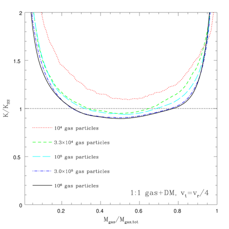
Figure 26: Comparison of final entropy profile for the 1:1 gas+DM small impact parameter merger simulated with various mass resolutions.

References

- Abadi et al. (2000) Abadi, M. G., Bower, R. G., & Navarro, J. F. 2000, MNRAS, 314, 759
- Babul et al. (2002) Babul, A., Balogh, M. L., Lewis, G. F., & Poole, G. B. 2002, MNRAS, 330, 329
- Balogh et al. (1999) Balogh, M. L., Babul, A., & Patton, D. R. 1999, MNRAS, 307, 463
- Balogh et al. (2001) Balogh, M. L., Pearce, F. R., Bower, R. G., & Kay, S. T. 2001, MNRAS, 326, 1228
- Benson (2005) Benson, A. J. 2005, MNRAS, 358, 551
- Benson et al. (2003) Benson, A. J., Bower, R. G., Frenk, C. S., Lacey, C. G., Baugh, C. M., & Cole, S. 2003, ApJ, 599, 38
- Binney & Tremaine (1987) Binney, J., & Tremaine, S. 1987, Princeton, NJ, Princeton University Press, 1987, 747, p. 204
- Borgani et al. (2004) Borgani, S., et al. 2004, MNRAS, 348, 1078
- Borgani et al. (2006) Borgani, S., et al. 2006, MNRAS, 367, 1641
- Bower (1997) Bower, R. G. 1997, MNRAS, 288, 355
- Bower et al. (2001) Bower, R. G., Benson, A. J., Lacey, C. G., Baugh, C. M., Cole, S., & Frenk, C. S. 2001, MNRAS, 325, 497
- Bower et al. (2006) Bower, R. G., Benson, A. J., Malbon, R., Helly, J. C., Frenk, C. S., Baugh, C. M., Cole, S., & Lacey, C. G. 2006, MNRAS, 370, 645
- Cavaliere et al. (1998) Cavaliere, A., Menci, N., & Tozzi, P. 1998, ApJ, 501, 493
- Cohn & White (2005) Cohn, J. D., & White, M. 2005, Astroparticle Physics, 24, 316
- Cole et al. (2000) Cole, S., Lacey, C. G., Baugh, C. M., & Frenk, C. S. 2000, MNRAS, 319, 168
- Dalla Vecchia et al. (2004) Dalla Vecchia, C., Bower, R. G., Theuns, T., Balogh, M. L., Mazzotta, P., & Frenk, C. S. 2004, MNRAS, 355, 995
- Dolag et al. (2004) Dolag, K., Jubelgas, M., Springel, V., Borgani, S., & Rasia, E. 2004, ApJ, 606, L97
- Donahue et al. (2006) Donahue, M., Horner, D. J., Cavagnolo, K. W., & Voit, G. M. 2006, ApJ, 643, 730
- Dos Santos & Doré (2002) Dos Santos, S., & Doré, O. 2002, A&A, 383, 450
- Eke et al. (2001) Eke, V. R., Navarro, J. F., & Steinmetz, M. 2001, ApJ, 554, 114
- Evrard & Henry (1991) Evrard, A. E., & Henry, J. P. 1991, ApJ, 383, 95
- Evrard et al. (1996) Evrard, A. E., Metzler, C. A., & Navarro, J. F. 1996, ApJ, 469, 494
- Faltenbacher et al. (2006) Faltenbacher, A., Hoffman, Y., Gottloeber, S., & Yepes, G. 2006, ArXiv Astrophysics e-prints, arXiv:astro-ph/0608304
- Frenk et al. (1999) Frenk, C. S., et al. 1999, ApJ, 525, 554
- Kaiser (1991) Kaiser, N. 1991, ApJ, 383, 104
- Kauffmann et al. (1999) Kauffmann, G., Colberg, J. M., Diaferio, A., & White, S. D. M. 1999, MNRAS, 303, 188
- Kazantzidis et al. (2004) Kazantzidis, S., Magorrian, J., & Moore, B. 2004, ApJ, 601, 37
- Khochfar & Burkert (2006) Khochfar, S., & Burkert, A. 2006, A&A, 445, 403
- Kravtsov et al. (2005) Kravtsov, A. V., Nagai, D., & Vikhlinin, A. A. 2005, ApJ, 625, 588
- Lacey & Cole (1993) Lacey, C., & Cole, S. 1993, MNRAS, 262, 627
- Lin et al. (2006) Lin, W. P., Jing, Y. P., Mao, S., Gao, L., & McCarthy, I. G. 2006, ApJ, 651, 636
- McCarthy et al. (2004) McCarthy, I. G., Balogh, M. L., Babul, A., Poole, G. B., & Horner, D. J. 2004, ApJ, 613, 811
- McCarthy et al. (2003) McCarthy, I. G., Holder, G. P., Babul, A., & Balogh, M. L. 2003, ApJ, 591, 526
- McCarthy et al. (2007) McCarthy, I. G., Babul, A., Bower, R. G., & Balogh, M. L., 2007, MNRAS, submitted
- Navarro et al. (1997) Navarro, J. F., Frenk, C. S., & White, S. D. M. 1997, ApJ, 490, 493
- Pfrommer et al. (2006) Pfrommer, C., Springel, V., Enßlin, T. A., & Jubelgas, M. 2006, MNRAS, 367, 113
- Piffaretti et al. (2005) Piffaretti, R., Jetzer, P., Kaastra, J. S., & Tamura, T. 2005, A&A, 433, 101
- Poole et al. (2006) Poole, G. B., Fardal, M. A., Babul, A., McCarthy, I. G., Quinn, T., & Wadsley, J. 2006, MNRAS, 373, 881
- Pratt et al. (2006) Pratt, G. W., Arnaud, M., & Pointecouteau, E. 2006, A&A, 446, 429
- Ricker & Sarazin (2001) Ricker, P. M., & Sarazin, C. L. 2001, ApJ, 561, 621
- Rowley et al. (2004) Rowley, D. R., Thomas, P. A., & Kay, S. T. 2004, MNRAS, 352, 508
- Shu (1992) Shu, F. H. 1992, Physics of Astrophysics, Vol. II, by Frank H. Shu. Published by University Science Books, ISBN 0-935702-65-2, 476pp, 1992., p. 215
- Sijacki & Springel (2006) Sijacki, D., & Springel, V. 2006, MNRAS, 366, 397
- Springel (2005) Springel, V. 2005, MNRAS, 364, 1105
- Springel & Hernquist (2002) Springel, V., & Hernquist, L. 2002, MNRAS, 333, 649
- Springel & Hernquist (2003) Springel, V., & Hernquist, L. 2003, MNRAS, 339, 312
- Springel et al. (2005) Springel, V., et al. 2005, Nature, 435, 629
- Tormen (1997) Tormen, G. 1997, MNRAS, 290, 411
- Tozzi & Norman (2001) Tozzi, P., & Norman, C. 2001, ApJ, 546, 63
- Vikhlinin et al. (2006) Vikhlinin, A., Kravtsov, A., Forman, W., Jones, C., Markevitch, M., Murray, S. S., & Van Speybroeck, L. 2006, ApJ, 640, 691
- Vitvitska et al. (2002) Vitvitska, M., Klypin, A. A., Kravtsov, A. V., Wechsler, R. H., Primack, J. R., & Bullock, J. S. 2002, ApJ, 581, 799
- Voit et al. (2003) Voit, G. M., Balogh, M. L., Bower, R. G., Lacey, C. G., & Bryan, G. L. 2003, ApJ, 593, 272
- Voit et al. (2002) Voit, G. M., Bryan, G. L., Balogh, M. L., & Bower, R. G. 2002, ApJ, 576, 601
- Voit et al. (2005) Voit, G. M., Kay, S. T., & Bryan, G. L. 2005, MNRAS, 364, 909
- Wang et al. (2005) Wang, H. Y., Jing, Y. P., Mao, S., & Kang, X. 2005, MNRAS, 364, 424
- Wu et al. (2000) Wu, K. K. S., Fabian, A. C., & Nulsen, P. E. J. 2000, MNRAS, 318, 889