Terrestrial Planet Formation Around Individual Stars Within Binary Star Systems

Abstract

We calculate herein the late stages of terrestrial planet accumulation around a solar type star that has a binary companion with semimajor axis larger than the terrestrial planet region. We perform more than one hundred simulations to survey binary parameter space and to account for sensitive dependence on initial conditions in these dynamical systems. As expected, sufficiently wide binaries leave the planet formation process largely unaffected. As a rough approximation, binary stars with periastron $q_{B}>10$ AU have minimal effect on terrestrial planet formation within $\sim 2$ AU of the primary, whereas binary stars with $q_{B}\lesssim$ 5 AU restrict terrestrial planet formation to within $\sim$ 1 AU of the primary star. Given the observed distribution of binary orbital elements for solar type primaries, we estimate that about 40 – 50 percent of the binary population is wide enough to allow terrestrial planet formation to take place unimpeded. The large number of simulations allows for us to determine the distribution of results — the distribution of plausible terrestrial planet systems — for effectively equivalent starting conditions. We present (rough) distributions for the number of planets, their masses, and their orbital elements.

1 Introduction

A binary star system is the most common result of the star formation process, at least for solar-type stars, and the question of planet formation in binaries is rapidly coming into focus. At least 30 of the first 170 extrasolar planets that have been detected are in so-called S-type orbits, which encircle one component of a main sequence binary/multiple star system (Eggenberger et al. 2004, Raghavan et al. 2006, Butler et al. 2006). This sample includes 3 systems — GJ 86 (Queloz et al. 2000), $\gamma$ Cephei (Hatzes et al. 2003), and HD 41004 (Zucker et al. 2004) — with stellar semimajor axes of only $\sim$ 20 AU, well within the region spanned by planets in our own Solar System. Five of these 30 planets orbit one member of a triple star system (Raghavan et al. 2006). One example is the planet HD 188753 Ab, which has a minimum mass of 1.14 times the mass of Jupiter, $M_{J}$, and was detected in a 3.35 day S-type orbit around a 1.06 $M_{\odot}$ star. A short-period binary star system (with a total mass of 1.63 $M_{\odot}$) orbits this host-star/planet system with a remarkably close periastron distance of $\sim$ 6 AU (Konacki 2005). The effects of the binary companion(s) on the formation of these planets remain unclear, especially from a theoretical perspective. The statistics of the observational data, however, suggest that binarity has an effect on planetary masses and orbits (Mazeh 2004, Eggenberger et al. 2004). The existence of terrestrial-mass planets in $\it{main}$ $\it{sequence}$ binary star systems remains observationally unconstrained. The Kepler Mission, set for launch in late 2008, has the potential to photometrically detect Earth-like planets in both single and binary star systems, and will help provide such constraints.

Some theoretical research on terrestrial planet formation in binary star systems has already been carried out. The growth stage from km-sized planetesimals to the formation of Moon- to Mars-sized bodies within a gaseous disk, via runaway and oligarchic growth, has been numerically simulated with favorable results in the $\alpha$ Centauri AB binary star system (Marzari and Scholl 2000) and the $\gamma$ Cephei binary/giant-planet system (Thebault et al. 2004). In each case, the combined effects of the stellar perturbations and gas drag lead to periastron alignment of the planetesimal population, thereby reducing the relative and collisional velocities and increasing the planetesimal accretion efficiency within $\sim$ 2.5 AU of the central star. Thebault et al. (2006) further examined this stage of planetesimal growth in binary star systems with stellar separations $a_{B}\leq$ 50 AU and eccentricities $e_{B}\leq$ 0.9. In addition to the damping of secular perturbations on planetesimals in the presence of gas drag, they found that the evolution is highly sensitive to the initial size-distribution of the bodies in the disk, and binary systems with $e_{B}\gtrsim$ 0 can inhibit runaway accretion within a disk of unequal-sized planetesimals.

The final stages of terrestrial planet formation - from planetary embryos to planets - have been modeled for $\alpha$ Centauri AB, the closest binary star system to the Sun (Barbieri et al. 2002, Quintana et al. 2002, Turrini et al. 2005). The G2 star $\alpha$ Cen A (1.1 M_⊙) and the K1 star $\alpha$ Cen B (0.91 M_⊙) are bound with a stellar separation of $a_{B}\sim$ 23.4 AU, a binary eccentricity $e_{B}\sim$ 0.52, and have a stellar periastron $q_{B}\equiv a_{B}(1-e_{B})\sim$ 11.2 AU. Various disk mass distributions around $\alpha$ Cen A were examined in Barbieri et al. (2002), and terrestrial planets formed in their simulations with semimajor axes within $\sim$ 1.6 AU of $\alpha$ Cen A. Quintana et al. (2002) performed 33 simulations using virtually the same initial disk mass distribution (the ‘bimodal’ model that is used in the simulations presented in this article), and examined a range of initial disk inclinations (0 to 60^∘ and also 180^∘) relative to the binary orbital plane for a disk centered around $\alpha$ Cen A, and performed a set of simulations with a disk centered around $\alpha$ Cen B coplanar to the stellar orbit. From 3 – 5 terrestrial planets formed around $\alpha$ Cen A in simulations for which the midplane of the disk was initially inclined by 30^∘ or less relative to the stellar orbit (Quintana et al. 2002, Quintana 2004), and from 2 – 5 planets formed around $\alpha$ Cen B (Quintana 2003). For comparison, growth from the same initial disk placed around the Sun with neither giant planets nor a stellar companion perturbing the system was simulated by Quintana et al. (2002). Material remained farther from the Sun, and accretion was much slower ($\sim$ 1 Gyr) compared with the aforementioned $\alpha$ Cen AB integrations ($\sim$ 200 Myr) and simulations of the Sun-Jupiter-Saturn system ($\sim$ 150 – 200 Myr), all of which began with virtually the same initial disk (Chambers 2001, Quintana & Lissauer 2006). These simulations show that giant and stellar companions not only truncate the disk, but hasten the accretion process by stirring up the planetary embryos to higher eccentricities and inclinations. Raymond et al. (2004) explored terrestrial planet growth around a Sun-like star with a Jupiter-like planet in a wide range of initial configurations (masses and orbits), and demonstrated that an eccentric Jupiter clears out material in the asteroid region much faster than a giant planet on a circular orbit.

The formation of planets in so-called P-type orbits which encircle both stars of a binary star system has also been investigated. Nelson & Papaloizou (2003) and Nelson (2003) studied the effects of a giant protoplanet within a viscous circumbinary disk (with the total mass of the stars and the protoplanet equal to 1 M_⊙), and found modes of evolution in which the protoplanet can remain in stable orbits, even around eccentric binary star systems. The final stages of terrestrial planet formation have been numerically simulated in P-type circumbinary orbits around binary stars with a total mass of 1 M_⊙, semimajor axes 0.05 AU $\leq a_{B}\leq$ 0.4 AU, and binary eccentricities $e_{B}\leq$ 0.8 (Quintana 2004, Lissauer et al. 2004, Quintana & Lissauer 2006). These simulations began with the same bimodal initial disk mass distribution as the model used in this article, and the final planetary systems were statistically compared to planetary systems formed in the Sun-Jupiter-Saturn system (which used the same starting disk conditions). Terrestrial planets similar to those in the Solar System formed around binary stars with apastra $Q_{B}\equiv a_{B}$(1 + $e_{B}$) $\lesssim$ 0.2 AU, whereas simulations of binaries with larger maximum separations resulted in fewer planets, especially interior to 1 AU of the binary star center of mass. Herein, we only consider terrestrial planet formation around a single main sequence star with a stellar companion, and aim to find similar constraints on the stellar masses and orbits that allow the formation of terrestrial planets similar to the Mercury-Venus-Earth-Mars system.

A related issue is that of the long term stability of planetary systems in binaries (after planet formation has been completed). Wiegert & Holman (1997) examined test particles around one and both stars in the $\alpha$ Cen AB system, and Holman & Wiegert (1999) explored the stability of orbits in and around (a wide range of) binary star systems. These two studies demonstrated that the stability regions are dependent on four parameters: the binary semimajor axis $a_{B}$, the binary eccentricity $e_{B}$, the inclination of the disk relative to the stellar orbit, and the stellar mass ratio $\mu\equiv M_{C}/(M_{\star}+M_{C})$, where $M_{\star}$ is the mass of the primary star and $M_{C}$ is the mass of the companion. Dynamical stability calculations of an Earth-like planet orbiting a Solar-mass (M_⊙) star with an intermediate mass companion ($M_{C}$ = 0.001 – 0.5 $M_{\odot}$) have shown that the regions of stability depend most sensitively on the binary periastron $q_{B}\equiv a_{B}(1-e_{B})$, for a given companion mass $M_{C}$ (David et al. 2003). These stability calculations, in conjunction with the observed distributions of binary orbital parameters (Duquennoy & Mayor 1991), indicate that $\sim$ 50% of all binary systems are wide enough so that Earth-like planets can remain stable for the age of the Solar System. Additionally, similar calculations of bodies in circumbinary orbits (Quintana & Lissauer 2006), along with the observed binary period distribution (David et al. 2003), indicate that approximately 10% of main sequence binary stars are close enough to each other to allow the formation and long-term stability of Earth-like planets. One goal of this paper is to provide an analogous constraint for planet $\it{formation}$ around individual stars in binary systems, i.e., find the fraction of binaries that allow for an entire system of terrestrial planets to form. For the sake of definiteness, we (somewhat arbitrarily) define a “complete” terrestrial planet system to be one that extends out to at least the present orbit of Mars, $\sim$ 1.5 AU, which encompasses the inner terrestrial planets in the Solar System and also the habitable zone of Sun-like stars (Kasting et al. 1993).

In this article, we present the results from a large survey ($\sim$ 120 numerical simulations) on the effects of a stellar companion on the final stages of terrestrial planet formation in S-type orbits around one component of a main sequence binary star system. We examine stellar mass ratios of $\mu$ = 1/3, 1/2, and 2/3 (for stars with masses of either 0.5 $M_{\odot}$ or 1 $M_{\odot}$), and the stellar orbital parameters ($a_{B}$, $e_{B}$) are varied such that the systems take on periastron values of $q_{B}$ = 5, 7.5, or 10 AU. Multiple simulations, usually 3 to 10, are performed for each binary star system with slight changes in the starting states in order to explore the sensitivity of the planet formation process to the initial conditions. In one case, we performed 30 integrations of a single system (with $q_{B}$ = 7.5 AU, $a_{B}$ = 10 AU, and $e_{B}$ = 0.25) to produce a large distribution of final planetary systems in order to quantify this chaotic effect. This paper is organized as follows. The orbital stability of test particles in S-type orbits in binary star systems is discussed in §2. The numerical model and initial conditions are presented in §3, and results of our planetary accretion simulations are presented and discussed in §4. We conclude in §5 with a summary of our results and their implications.

2 Orbital Stability

Prior to examining planetary accretion in binaries, we briefly consider the stability of test particles in the binary systems of interest. In approximate terms, if a binary is wide enough so that test particles in orbit about the primary remain largely unperturbed over a time span of $\sim 100$ Myr (characteristic of terrestrial planet formation), one would not expect the binary to have a large impact on planet formation. The regions of orbital stability of planets in S-type orbits have been investigated previously for a wide range of binary star systems (Holman & Wiegert 1999, David et al. 2003). Holman & Wiegert (1999) performed a dynamical analysis for stellar mass ratios in the range 0.1 $\leq\mu\leq$ 0.9, and for binary eccentricities 0 $\leq e_{B}\leq$ 0.8. In their study, test particles were placed in the binary orbital plane between 0.02 $a_{B}$ and 0.5 $a_{B}$ at eight equally spaced longitudes per semimajor axis, and the system was evolved forward in time for 10⁴ binary periods. The outermost stable orbit to the primary star for which all eight particles survived (which they refer to as the ‘critical semimajor axis’, $a_{c}$) was determined for each system.

We have performed analogous test particle simulations for the binary star systems examined in this article, which include equal mass ($\mu$ = 0.5) binary stars (with eccentricities 0 $\leq e_{B}\leq$ 0.875), and binary systems with $\mu$ = 1/3 or 2/3 (where $e_{B}$ = 0.25 in each case). Test particles were placed between 0.02 $a_{B}$ and 0.5 $a_{B}$ (with increments of 0.01 $a_{B}$) at eight equally spaced longitudes per semimajor axis. We use a ‘wide-binary’ symplectic algorithm developed by Chambers et al. (2002) for these and subsequent accretion simulations. This algorithm is based on the mapping method of Wisdom & Holman (1991), and was designed to calculate the evolution of particles/bodies around a central star with a massive companion perturbing the primary star/disk system. Each system was followed for 10⁶ binary orbits, and the critical semimajor axis (for which all eight particles remained in the system) was calculated and is given in Table 1. Note that some of the systems used here have values of $e_{B}$ in between those examined in Holman & Weigert (1999), and upon extrapolation the results presented in Table 1 are consistent with their study.

3 Numerical Model and Initial Conditions

Each simulation begins with a disk of planetesimals and planetary embryos centered around what we will refer to as the primary star (even though for most simulations the stars have equal masses, and in one set of runs the planetesimals and embryos encircle the lower mass star), with the midplane of the disk coplanar to the stellar orbit, and the binary companion in an orbit exterior to the terrestrial planet region. These simulations use an initial disk composed of planetesimals and embryos with masses and orbits virtually identical to those used in previous simulations of terrestrial planet formation in the Sun-Jupiter-Saturn System, in particular, the model of Chambers (2001) that was most successful in reproducing the terrestrial planets in our Solar System. Although this formulation is not complete, nor definitive, it provides a model that reproduces our terrestrial planet system (albeit with somewhat larger eccentricities) and can thus be used as a reference point. By performing a large ensemble of analogous simulations in binary systems with varying orbital elements, we can assess the effects of binarity on the planet formation process.

The disk is composed of Moon- to Mars-sized rocky bodies which are assumed to have already formed from a disk of gas and dust. In particular, 14 planetary embryos (each 0.0933 times the mass of the Earth, M_⊕) compose half of the disk mass, while the remaining mass is distributed equally among 140 planetesimals (each with a mass of 0.00933 M_⊕), providing a total disk mass of $\sim$ 2.6 M_⊕. The initial radial extent of the disk is between 0.36 AU – 2.05 AU of the primary star, and the radius of each body is calculated assuming a material density of 3 g cm^-3. The protoplanets began with initial eccentricities of $e\leq$ 0.01, inclinations $i\leq$ 0.5^∘, and specific initial orbital elements were chosen at random from specified ranges; the same set of randomly selected values was used for all simulations.

The ‘wide-binary’ algorithm that we use follows the evolution of each body in the disk subject to gravitational perturbations from both stars, and to gravitational interactions and completely inelastic collisions with other bodies in the disk (Chambers et al. 2002). Material that is not accreted onto growing planets may be lost from the system by either orbiting too close to the central star (for the simulations presented herein, planetesimals/embryos are removed when their periastron $\leq$ 0.1 AU), or if it is ejected from the system (if its trajectory exceeds a distance comparable to the binary semimajor axis). A time-step of 7 days is used, and the evolution of each system is followed for 200 – 500 Myr. For a discussion on the validity of using a 7-day time-step for this accretion disk, see Section 2.2 of Quintana & Lissauer (2006).

Many of our simulations began with binary stars on highly eccentric orbits, which would perturb disk material into more elliptical orbits than is considered in our chosen initial conditions. One might worry that this mismatch in initial conditions could produce a systematic bias in our results. This issue was investigated in Appendix B of Quintana & Lissauer (2006), in which the standard bimodal disk (as previously described) was centered around close binary stars. It was shown that beginning the protoplanets with the appropriate nested elliptical orbits, rather than in nearly circular orbits, did not impact the resulting planetary systems in a statistically significant manner. In other words, the systematic effect from the differing initial eccentricities of bodies in each disk on the final planet systems that form (in otherwise identical systems) were comparable to or smaller than the effects resulting from chaos. These results were also consistent with test particle simulations in eccentric binary star systems performed by Pichardo et al. (2005).

We examine binary star systems with stellar mass ratios $\mu\equiv M_{C}/(M_{\star}+M_{C})$ = 1/3, 1/2, or 2/3, where $M_{\star}$ is the mass of the primary star and $M_{C}$ is the mass of the companion. Table 2 displays the stellar parameters used in our accretion simulations, grouped into four sets according to the stellar masses involved. The majority of our simulations begin with equal mass stars ($\mu$ = 1/2) of either $M_{\star}$ = $M_{C}$ = 0.5 M_⊙ (Set A) or $M_{\star}$ = $M_{C}$ = 1 M_⊙ (Set B). In the simulations of Set C, the primary star (the one the disk is centered around) is more massive, $M_{\star}$ = 1 M_⊙ and $M_{C}$ = 0.5 M_⊙ ($\mu$ = 1/3). In Set D, the primary star is smaller, $M_{\star}$ = 0.5 M_⊙ and $M_{C}$ = 1 M_⊙ ($\mu$ = 2/3). The stellar semimajor axis $a_{B}$ and binary eccentricity $e_{B}$ are varied such that the binary periastron takes one of the three values $q_{B}$ = 5, 7.5, or 10 AU (see columns 2 – 4 of Table 2). Note that binary systems with much wider periastra would have little effect on terrestrial planet formation, whereas systems with smaller periastra would completely destroy the initial disk of planetesimals. The binary stars are separated by $a_{B}$ = 10, 13$\frac{1}{3}$, 20, or 40 AU, and the eccentricities are varied in the range 0 $\leq e_{B}\leq$ 0.875. The fifth column of Table 2 gives the outermost stable orbit for each system, $a_{c}$ (expressed here in AU), as described in the previous section. The largest semimajor axis for which particles can be stable in any of the systems that we explore is 2.6 AU (Table 2), we therefore omit giant planets analogous to those in the Solar System (which orbit beyond 5 AU) in our integrations.

For our accretion simulations, our exploration of parameter space has two coupled goals. On one hand, we want to determine the effects of the binary orbital elements on the final terrestrial planet systems produced. On the other hand, for a given binary configuration, we want to explore the distribution of possible resulting planetary systems (where the results must be described in terms of a distribution due to the sensitive dependence on the initial conditions). Toward these ends, we have performed from 3 – 30 integrations (last column in Table 2) for each binary star configuration ($\mu$, $a_{B}$, and $e_{B}$) considered herein, with small differences in the initial conditions: a single planetesimal near 0.5, 1, or 1.5 AU is moved forward along its orbit by a small amount (1 – 9 meters) prior to the integration. Ideally, of course, one would perform larger numbers of integrations to more fully sample the distributions of results, but computer resources limit our sample size.

4 Planetary Accretion Simulations

This section presents the results of our numerical simulations. We first consider the chaotic nature of the integrations (§4.1) and discuss how sensitive dependence on initial conditions affects the nature of our results. In §4.2, we present a broad overview of our simulations by showing typical sequences of evolution and general trends emerging in the results. We focus on the properties of final planetary systems in §4.3, where such properties are described in terms of distributions.

4.1 Chaotic Effects

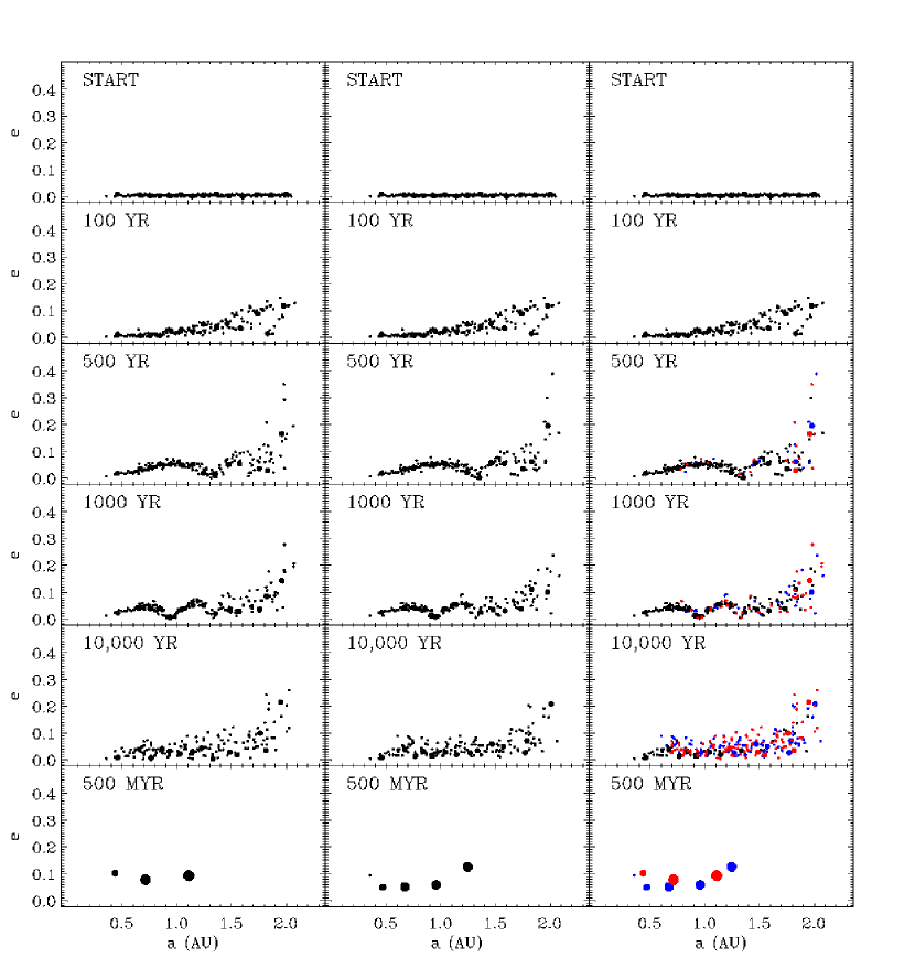
Figure 1: The temporal evolution of two simulations, each with $a_{B}$ = 10 AU, $e_{B}$ = 0.25, and equal mass stars of 1 M_⊙, is shown in the first two columns. The only difference between these two simulations at the start of the integration is that one planetesimal near 1 AU (in the second run) is shifted forward by 1 meter along its orbit. The third column overlays the two systems at the corresponding time in order to demonstrate the divergence of initially nearby orbits. The bodies in the disk are represented by circles whose sizes are proportional to the physical sizes of the bodies, and whose locations show the orbital semimajor axes and eccentricities of the represented bodies relative to the central star. In the third column, bodies for which $(e_{p_{1}}-e_{p_{2}})^{2}+(a_{p_{1}}-a_{p_{2}})^{2}>$ 0.001, where $e_{p}$ and $a_{p}$ are the eccentricity and semimajor axis of each planetesimal/embyro, are plotted in red (for the bodies from the first column) and in blue (for the corresponding bodies in the second column). Note that while these systems seem qualitatively similar at early times, the two systems begin to diverge within 500 years of the simulation. The small change in the initial conditions ultimately leads to the formation of two very different planetary systems, 3 planets versus 5, as shown in the final row.

Before comparing the results of terrestrial planet growth within various binary star systems, it is worthwhile to take a closer look at the stochastic nature of these $N$-body simulations, and keep in mind throughout this study: “Long term integrations are not ephemerides, but probes of qualitative and statistical properties of the orbits …” (Saha et al. 1997). To demonstrate the sensitive dependence on the initial conditions, Figure 1 shows the evolution of two nearly identical simulations (with $a_{B}$ = 10 AU, $e_{B}$ = 0.25, and $M_{\star}$ = $M_{C}$ = 1 M_⊙) that differ only in a 1 meter shift of one planetesimal near 1 AU prior to the integration. Each panel shows the eccentricity of each body in the disk as a function of semimajor axis at the specified time, and the radius of each symbol is proportional to the radius of the body that it represents. The first two columns show the temporal evolution from each simulation, and the third column plots the discrepancy between the two systems at the corresponding simulation time: planetesimals/embryos from columns one and two with orbits which diverged in $(a,e)$ space by more than 0.001 are shown in red and in blue, respectively. At 100 years into the simulation, the two disks shown in Figure 1 are virtually identical. Although there are no ejections nor collisions within the first 500 years of either simulation, the bodies in the disk are dynamically excited, especially towards the outer edge of the disk, and begin to exhibit chaotic behavior. The general behavior of the disk is similar among the two systems, yet the stochastic nature leads to remarkably different final planetary systems.

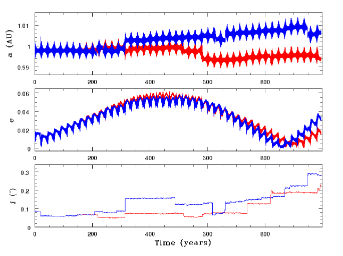
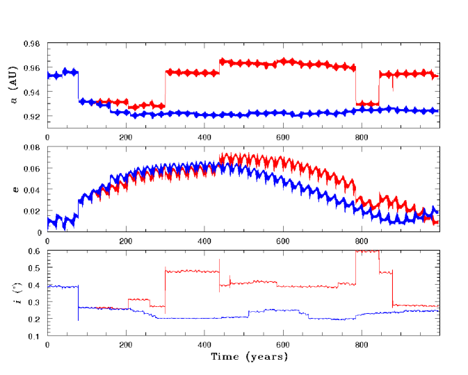
Figure 2: The time evolution of the semimajor axis ($a_{p}$), eccentricity ($e_{p}$), and inclination ($i_{p}$) is shown for a planetesimal on an initial orbit near 1 AU (upper 3 panels), and for another planetesimal that began near 0.95 AU (lower 3 panels), from the first 1000 years of the two simulations shown in Figure 1. (a) In the top figure, the initial orbits of the two planetesimals differ by 1 meter in their mean anomoly, while all other system parameters are identical. (b) In the bottom figure, the two planetesimals began on identical orbits near 0.95 AU (also shown in red and blue). The chaotic behavior of these systems is apparent early in the simulations, and the orbital elements of nearby trajectories diverge with Lyapunov times of $\sim$ 100 – 200 years.

Figures 2a and 2b each show the orbital elements of a single planetesimal from the two simulations presented in Figure 1. The semimajor axis ($a_{p}$), eccentricity ($e_{p}$), and inclination relative to the binary orbital plane ($i_{p}$) are shown as a function of time for the first 1000 years of the integrations. In Figure 2a, the two planetesimals (shown in red and in blue) began with the same semimajor axis near 1 AU, and differed only by a 1 meter shift in their mean anomaly. The two planetesimals shown in Figure 2b, from the same two simulations as the planetesimals in Figure 2a, began with identical initial orbits near 0.95 AU. The values of each element oscillate with time due to the combined effect of the stellar and planetary perturbations, and the orbits of two planetesimals clearly diverge from one another on timescales longer than their short period oscillations. The divergence between the simulations is mainly due to discrete events, i.e. close encounters between planetesimals/embryos, and the Lyapunov time for these $N$-body systems (where $N$ = 156) is of order $10^{2}$ years. In Figure 2a, the planetesimal shown in red was ultimately ejected at 6.8 Myr into the first integration, while the planetesimal shown in blue fell to within 0.1 AU of the central star at 10.6 Myr into the second integration. In Figure 2b, the planetesimal shown in red collided with another planetesimal at 1.4 Myr, and this more massive body was later accreted by an embryo at 58 Myr. The planetesimal shown in blue in Figure 2b, however, was swept up by a larger embryo at 47.6 Myr into the simulation. Although small differences in initial conditions (among an otherwise identical system) can ultimately lead to the formation of entirely different terrestrial planet systems (number, masses, and orbits, etc.), the early evolution of the disk is similar among systems with the same binary star parameters, and there are clear trends in the final planetary systems that form (as presented and discussed in the next two subsections).

4.2 Overview of Results

Table 3 displays, for each binary star configuration, a set of statistics developed to help quantify the final planetary systems formed. Each ($\mu$, $a_{B}$, $e_{B}$) configuration is listed in column 1, and the number of runs performed for each configuration are given in column 2. Columns 3 – 13 are defined as follows (see Chambers 2001, Quintana et al. 2002, and Quintana & Lissauer 2006 for mathematical descriptions of most of these statistics). Note that, with the exception of column 5, only the average value of each statistic is given for each set.

(3)

The average number of planets, $N_{p}$, at least as massive as the planet Mercury ($\sim$ 0.06 M_⊕), that form in the system. Note that each of the 14 planetary embryos in the initial disk satisfy this mass requirement, as do bodies consisting of at least 7 planetesimals.

(4)

The average number of minor planets, $N_{m}$, less massive than the planet Mercury that remain in the final system.

(5)

The maximum semimajor axis of the final planets, $a_{p_{max}}$.

(6)

The average value of the ratio of the maximum semimajor axis to the outermost stable orbit of the system, $a_{p_{max}}$/$a_{c}$.

(7)

The maximum apastron of the final planets, $Q_{p}\equiv$ $a_{p}$(1 + $e_{p}$).

(8)

The average value of the ratio of the maximum apastron $Q_{p}$ to the binary periastron $q_{B}\equiv$ $a_{B}$(1 – $e_{B}$).

(9)

The fraction of the final mass in the largest planet, $S_{m}$.

(10)

The percentage of the initial mass that was lost, $m_{l_{\star}}$, due to close encounters ($\leq$ 0.1 AU) with the primary star.

(11)

The percentage of the initial mass that was ejected from the system without passing within 0.1 AU of the primary star, $m_{l_{\infty}}$.

(12)

The total mechanical (kinetic + potential) energy per unit mass for the planets remaining at the end of a simulation, $E$, normalized by $E_{0}$, the energy per unit mass of the disk bodies at the beginning of the integration.

(13)

The angular momentum per unit mass of the final planets, $L$, normalized by $L_{0}$, the angular momentum per unit mass of the initial system.

For comparison, following the results from Sets A - D are analogous statistics for the following systems: the terrestrial planets Mercury-Venus-Earth-Mars in the Solar System (‘MVEM’, of which only three are actual observables); the averaged values for 31 accretion simulations in the Sun-Jupiter-Saturn system (‘SJS$\_{\rm{ave}}$’, Chambers 2001, Quintana & Lissauer 2006); the averaged values from a set of accretion simulations around the Sun with neither giant planets nor a stellar companion perturbing the system (‘Sun$\_{\rm{ave}}$’, Quintana et al. 2002); the averaged values for the planets formed within 2 AU of the Sun-only simulations (‘Sun$\_{\rm{ave}}$ ($a<$ 2 AU)’, Quintana et al. 2002); and the averaged values for the planetary systems formed around $\alpha$ Cen A in simulations for which the disk began coplanar ($i=$ 0^∘) to the $\alpha$ Cen AB binary orbital plane (‘$\alpha$ Cen ($i=$ 0^∘)’, Quintana et al. 2002).

Table 3 shows both the striking uniformity of (many of) these statistical measures, in spite of the great diversity of stellar configurations under consideration, and the systematic variation of the output measures with initial conditions. For example, column 8 shows that terrestrial planet systems have a “nearly constant” size, measured as a fraction of binary periastron. On one hand, this size ratio lies in the range 0.12 to 0.23 for each set of simulations. On the other hand, this size ratio clearly varies systematically with variations in the class of initial conditions. Of course, the ratio varies from system to system within the same class of starting conditions. Similar behavior occurs for all of these statistical measures: they all have well-defined characteristic values for the entire (diverse) set of systems under consideration, they all vary systematically with the class of initial conditions, and they all vary stochastically from case to case for systems within the same (effectively equivalent) class of initial conditions.

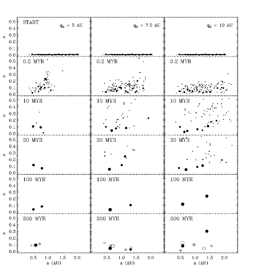
Figure 3: The temporal evolution of three systems from Set A is shown here, with each body in the disk represented by black solid circles (with symbol sizes proportional to planet sizes). These three simulations each begin with equal mass stars of 0.5 M_⊙ and semimajor axis $a_{B}$ = 20 AU. The simulations differ in their stellar eccentricities (and therefore periastra): $e_{B}$ = 0.75 and $q_{B}$ = 5 AU (first column), $e_{B}$ = 0.625 and $q_{B}$ = 7.5 AU (middle column), and $e_{B}$ = 0.5 and $q_{B}$ = 10 AU (third column). The disk is clearly truncated in the $q_{B}$ = 5 AU and 7 AU simulations, but still dynamically excited in each case. The amount of mass that is lost (averaged for each system) is approximately 71% ($q_{B}$ = 5 AU), 48% ($q_{B}$ = 7.5 AU), and 33% ($q_{B}$ = 10 AU). The final planets formed from two additional realizations of each system (with the same stellar parameters) are shown in the last row with gray and open circles; their early evolution (not shown) has similar trends as the simulation shown with black solid symbols.

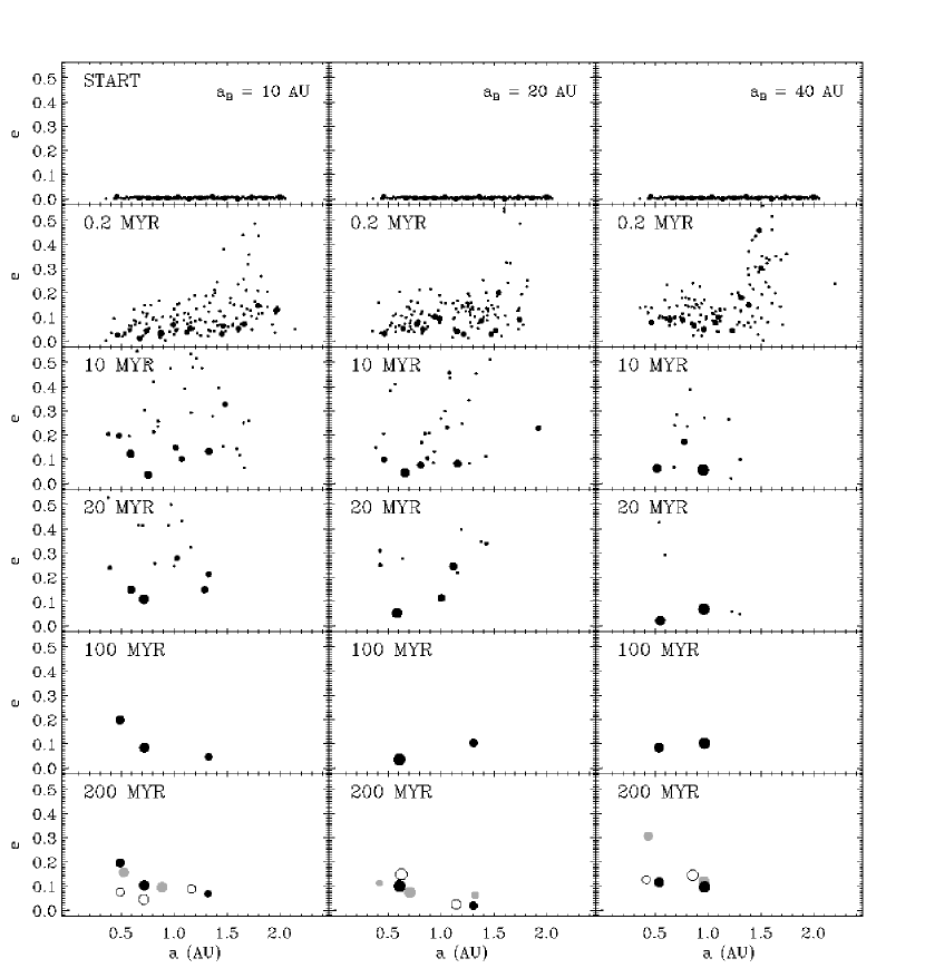
Figure 4: The temporal evolution of the bodies in the disk from three simulations of Set A ($M_{\star}$ = $M_{C}$ = 0.5 M_⊙), each of which began with a binary periastron of $q_{B}$ = 7.5 AU, are represented in each column with black filled circles. The simulations differ in the stellar semimajor axes $a_{B}$ and eccentricities $e_{B}$. In the first column, $a_{B}$ = 10 AU and $e_{B}$ = 0.25, in the middle column $a_{B}$ = 20 AU and $e_{B}$ = 0.625, and in the third column $a_{B}$ = 40 AU and $e_{B}$ = 0.8125. The bottom row displays the results of two additional simulations (shown by gray and open circles) which began with the same stellar parameters. See Figure 3 for an explanation of the symbols. Early in each simulation, many of the planetesimals near the outer edge of the disk are lost from the system, as are the more massive embryos in simulations that begin with larger $a_{B}$ and $e_{B}$. The total mass loss from the three integrations is comparable, $\sim$ 50%, although most of the mass that is lost from the more eccentric binary star systems (middle and third columns) typically ends up being removed by passing too close (within 0.1 AU) to the central star.

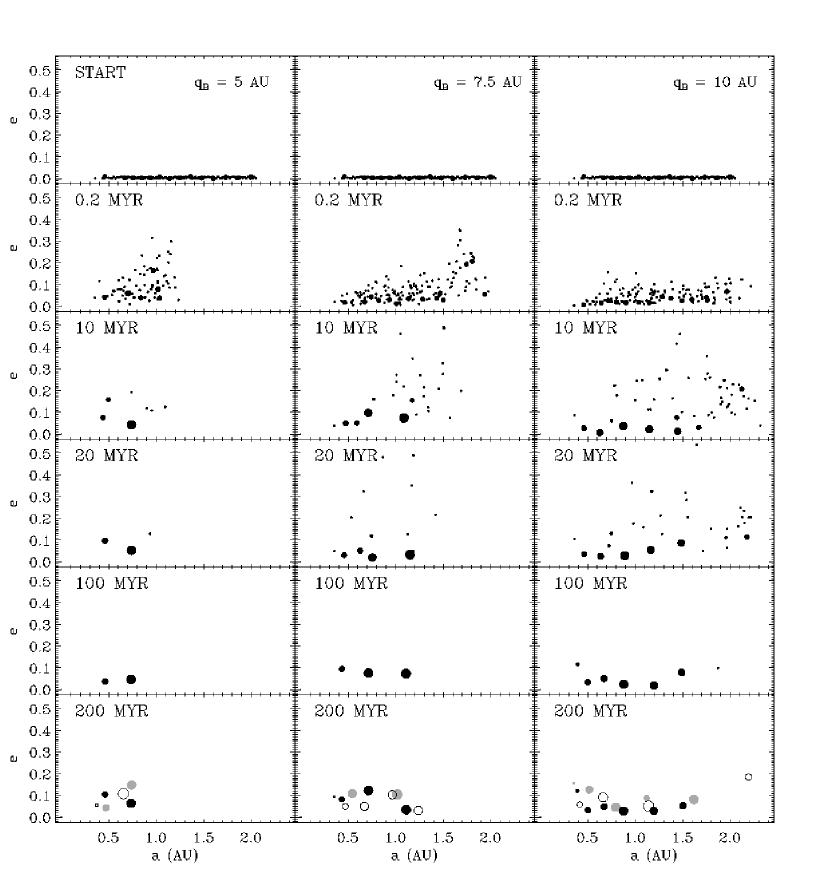
Figure 5: The temporal evolution of the bodies in the disk from three simulations of Set B ($M_{\star}$ = $M_{C}$ = 1 M_⊙), each of which begin with $a_{B}$ = 10 AU, is shown in each column with black filled circles. These simulations differ in the binary eccentricity and periastra: $e_{B}$ = 0.5 and $q_{B}$ = 5 AU (left column), $e_{B}$ = 0.25 and $q_{B}$ = 7.5 AU (middle column), and $e_{B}$ = 0 and $q_{B}$ = 10 AU (right column). The bottom row also displays the results of two additional simulations (shown by gray and open circles) using the same stellar parameters. See Figure 3 for the explanation of the symbols. These simulations display similar accretion time scales, and result in similar final planetary systems, as analogous simulations from Set A which have the same stellar mass ratio $\mu$ = 0.5, but consist of equal mass stars of 0.5 M_⊙. The bodies in the disk in Set B, however, are slightly less perturbed than those in Set A due to the smaller mass ratio of the planetesimals/embryos to the stars, which leads to systems with slightly larger radial extents than those formed in Set A.

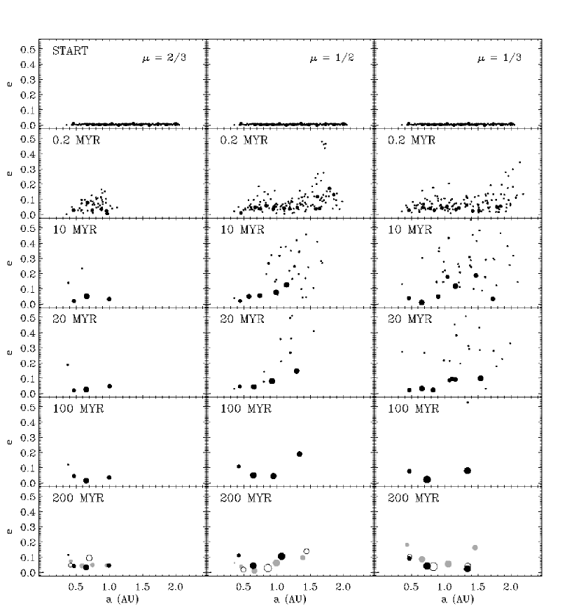
Figure 6: The temporal evolution of three simulations (shown in each column by black filled circles) with different stellar mass ratios, but the same orbital parameters: $q_{B}$ = 7.5 AU, $a_{B}$ = 10 AU, and $e_{B}$ = 0.25. The left column shows a system with $\mu$ = 2/3 ($M_{\star}$ = 0.5 M_⊙ and $M_{C}$ = 1 M_⊙), the system in the middle column has $\mu$ = 1/2 ($M_{\star}$ = $M_{C}$ = 1 M_⊙), and the third column shows $\mu$ = 1/3 (in which $M_{\star}$ = 1 M_⊙ and $M_{C}$ = 0.5 M_⊙). The bottom row also displays the results of two additional simulations (shown by gray and open circles) using the same stellar parameters. See Figure 3 for the explanation of the symbols. Although the amount of mass that is lost in these systems is quite different (an average of 72%, 40%, and 25% for columns 1, 2, and 3, respectively), the fraction of mass in the largest planet within each system is comparable, $\sim$ 50% ($S_{m}\sim$ 0.5) on average.

A visual comparison of the effects from various binary stars on the evolution of the disk of planetary embryos is given in Figures 3 – 6, each of which provides a side-by-side view of three simulations that have two of the four stellar parameters ($\mu$, $a_{B}$, $e_{B}$, $q_{B}$) in common. Figure 3 shows the evolution of three systems from Set A, each with $\mu$ = 0.5 ($M_{\star}$ = $M_{C}$ = 0.5 M_⊙) and $a_{B}$ = 20 AU. The simulations differ only in the stellar eccentricities (and therefore periastra): $e_{B}$ = 0.75 and $q_{B}$ = 5 AU (first column), $e_{B}$ = 0.625 and $q_{B}$ = 7.5 AU (middle column), and $e_{B}$ = 0.5 and $q_{B}$ = 10 AU (third column). The temporal evolution of a single simulation is shown with black solid circles which represent (and are proportional to) the bodies in the disk. Additionally, the last row shows the final planetary systems that formed in 2 other realizations of the same system (shown with gray and open circles in Figures 3 – 6). In the first two columns of Figure 3, binary systems with $q_{B}$ = 5 AU and 7 AU, the stellar companion truncates the disk to within 2 AU early in the simulation. The high binary star eccentricities stir up both the planetesimals and embryos, especially towards the outer edge of the disk. Among the three realizations of the $q_{B}$ = 5 AU system, 40% of the initial mass on average was perturbed to within 0.1 AU of the central star, and an average of 31% of the initial disk mass was ejected from the system (see columns 10 and 11 of Table 3). The remaining mass was accreted into 1 or 2 final planets, with semimajor axes $a_{p}\lesssim$ 0.7 AU, on timescales of $\sim$ 20 – 50 Myr.

The middle column of Figure 3 shows the $q_{B}$ = 7.5 AU ($e_{B}$ = 0.625) system, in which an average of $\sim$ 39% of the material was lost into the central star, and only 9% of the initial mass was ejected from the system. Most of the accretion was complete by $\sim$ 100 Myr, resulting in the formation of 2 – 3 planets with $a_{p}\lesssim$ 1.3 AU (the largest apastron of any planet in the set was $Q_{p}$ = 1.4 AU). In the $q_{B}$ = 10 AU (and $e_{B}$ = 0.5) simulations, shown in the third column of Figure 3, the eccentricities of the bodies in the disk are perturbed to high values, while the disk extends to beyond 2 AU within the first 20 Myr. In these runs, an average of $\sim$ 31% of the initial mass is lost into the primary star, $\sim$ 2% is ejected, and 2 or 3 planets remain within $Q_{p}\lesssim$ 1.8 AU. The fraction of mass that composes the largest planet, $S_{m}$ (column 9 of Table 3), decreases with increasing $q_{B}$ (from 0.95 – 0.53 in the systems shown in Figure 3), and is anti-correlated with the number of final planets that form. The magnitude of the specific energy of the $q_{B}$ = 5, 7.5, and 10 AU systems increase by 76%, 43%, and 31%, respectively, while the specific angular momentum of these systems decrease by 29%, 19%, and 13% from their original values (columns 12 and 13 of Table 3).

Figure 4 shows three simulations from Set A with the same stellar periastron $q_{B}$ = 7.5 AU, but with differing values of ($a_{B}$, $e_{B}$). In the first column, in which $a_{B}$ = 10 AU and $e_{B}$ = 0.25, the planetesimals are highly excited, yet most of the larger embryos in the disk remain with $e_{p}$ $\lesssim$ 0.1 within the first few million years. In the middle and final column, in which the semimajor axis and the eccentricity ($a_{B}$, $e_{B}$) are both increased to (20 AU, 0.625) and (40 AU, 0.8125), respectively, the more massive embryos are also excited to high values of $e_{p}$. The total mass that was lost is comparable among the three simulations, and also among the additional realizations of the three systems shown in Figure 4: 49% on average when $a_{B}$ = 10 AU, 48% for $a_{B}$ = 20 AU, and 52% for $a_{B}$ = 40 AU. The more eccentric binary stars tend to stir up the outer edge of the disk such that most of the mass that is lost is perturbed to within 0.1 AU of the primary star; approximately 82% and 65% of the mass that was lost in the second ($a_{B}$ = 20 AU, $e_{B}$ = 0.625) and third ($a_{B}$ = 40 AU, $e_{B}$ = 0.8125) simulations was perturbed into the central star, whereas 80% of the mass lost in the simulation shown in the first panel ($a_{B}$ = 10 AU, $e_{B}$ = 0.25) was ejected from the system. Although the total change in energy and angular momentum of each system is comparable, fewer planets form, with the outermost planet closer to the central star, for binary stars on more eccentric orbits. The effect of a more eccentric binary star system for a given $q_{B}$ is typically a more diverse set of planetary systems, which was also the case for terrestrial planet formation within a circumbinary disk surrounding highly eccentric close binary stars (but in that case the apastron value was the pertinent parameter, Quintana & Lissauer 2006).

Three simulations from Set B ($M_{\star}$ = $M_{C}$ = 1.0 M_⊙) with $a_{B}$ = 10 AU (and differing $e_{B}$ and $q_{B}$) are shown in Figure 5. Although the binary stars in Set B are each twice as massive as those in Set A, the mass ratio is the same ($\mu$ = 0.5) and for a given ($a_{B}$, $e_{B}$), or $q_{B}$, the simulations display similar trends (Figure 5) as those from Set A (Figure 3). Note that only three final planetary systems (from three realizations chosen at random) are shown in the last row of each column in Figures 5 and 6, even though from 10 – 30 integrations were performed, in order to demonstrate with clarity the diversity of final planets among each set. For simulations with $q_{B}$ = 5 AU ($a_{B}$ = 10 AU and $e_{B}$ = 0.5), an average of 36% of the initial disk mass was lost to the central star, and 29% was ejected from the system. In the 10 runs of this system, from 1 – 2 terrestrial-mass planets formed with $Q_{p}<$ 1 AU of the central star. We performed an ensemble of 30 integrations for a system with $q_{B}$ = 7.5 AU, $a_{B}$ = 10 AU, and $e_{B}$ = 0.25 system, three of which are shown in the middle column of Figure 5. The average percentage of mass that falls within 0.1 AU of the star is 10%, consistent with the analogous runs from Set A, whereas the mass perturbed out of the system is somewhat less, 30% on average. Within the first 50 Myr, from 2 – 5 planets at least as massive as Mercury have accreted, with 2 – 5 planetesimals remaining in each system on highly eccentric orbits. From 1 – 4 final terrestrial planets formed (with an average of 2.8) with $Q_{p}\lesssim$ 1.8 AU of the primary star. The somewhat less mass that is lost in Set B compared with an identical orbital parameter system from Set A can be expected, as although stellar perturbations are directly scaled, planetary perturbations are relatively less significant in Set B since the mass ratio of the planet to the star is smaller, which results in less internal excitation (see Appendix C of Quintana & Lissauer 2006 for a discussion of scaling planetary accretion simulations). In simulations from Set B with larger periastra of $q_{B}$ = 10 AU ($a_{B}$ = 10 AU, $e_{B}$ = 0), such as those shown in the third column of Figure 5, from 2 – 5 planets form with semimajor axes that encompass the full range of the initial disk, and even beyond 2 AU (one planet remained with $Q_{p}$ = 2.78), with 26% of the initial disk mass lost via ejection. The disk is slightly more truncated in simulations from Set B with $q_{B}$ = 10 AU, $a_{B}$ = 40 AU and $e_{B}$ = 0.75 (not shown), and from 1 – 4 planets accreted with $Q_{p}<$ 2 AU by the end of these integrations.

Figure 6 presents the evolution of three simulations with the same orbital parameters, $a_{B}$ = 10 AU and $e_{B}$ = 0.25 ($q_{B}$ = 7.5 AU), but examines the effect of different stellar mass ratios. In the first column, the central star has a mass of 0.5 M_⊙, and a 1 M_⊙ star perturbs the disk. Among this set, an average of 72% of the initial disk mass is cleared out (all of it into interstellar space), and the remaining mass is accreted into 2 – 4 planets with $Q_{p}\lesssim$ 1.1 AU. The middle column shows three additional simulations from the $q_{B}$ = 7.5 AU ($a_{B}$ = 10 AU, $e_{B}$ = 0.25) system from Set B that is shown in the middle column of Figure 5, in which $\sim$ 40% of the initial mass is lost on average. The final column shows a simulation with the disk centered around a 1 M_⊙ star with a 0.5 M_⊙ stellar companion. In this set of runs with $\mu$ = 1/3, an average of 26% of the initial disk mass is lost (most of it is perturbed to within 0.1 AU the central star), and 3 or 4 planets accrete with $Q_{p}\lesssim$ 1.8 AU in each simulation. This configuration statistically has the same effect on the disk and the resulting planets as Jupiter and Saturn do in analogous simulations of the Solar System (Chambers et al. 2001, Quintana & Lissauer 2006). Note that the temporal evolution of most individual simulations from Sets A and B are presented in Quintana (2004).

4.3 Final Planetary Systems

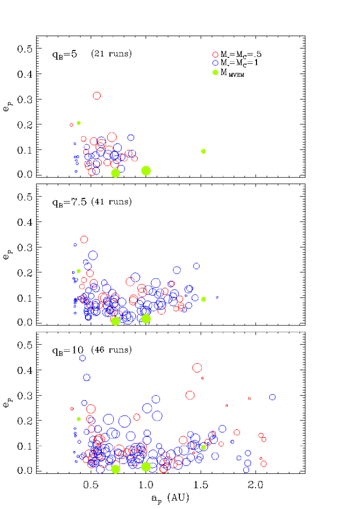
Figure 7: The eccentricity as a function of semimajor axis is shown for all of the final planets formed in equal-mass binary star systems with $q_{B}$ = 5 AU (top panel), $q_{B}$ = 7.5 AU (middle panel), and $q_{B}$ = 10 AU (bottom panel). The radius of each symbol is proportional to the body that it represents, and the terrestrial planets in our Solar System (at the J2000 epoch) are represented by green filled circles in each panel for comparison. The red symbols represent binary systems from Set A with $M_{\star}$ = $M_{C}$ = 0.5 M_⊙, while the blue symbols represent systems from Set B with $M_{\star}$ = $M_{C}$ = 1.0 M_⊙. The two distributions for each $q_{B}$ are comparable, although planetary perturbations in the Set B simulations are relatively smaller than those of Set A due to the smaller ratio of planet-to-star mass, which results in less internal excitation. This effect is evident in the larger number of planetesimals that have remained close to the central star in the Set B simulations shown in each panel.

As described in the previous section, the stellar mass ratio and the periastron distance strongly influence where terrestrial planets can form in binary star systems. The effect of $q_{B}$ on the distribution of final planetary system parameters (i.e., number, masses, etc.) is further explored in this section. Figure 7 displays the distribution of planetary eccentricities and semimajor axes for all of the final planets formed in equal-mass binary systems, with symbol sizes proportional to planet sizes, with $q_{B}$ = 5 AU (top panel), 7.5 AU (middle panel), and 10 AU (lower panel). Systems with $M_{\star}$ = $M_{C}$ = 0.5 M_⊙ (Set A) are represented in red, while systems with $M_{\star}$ = $M_{C}$ = 1.0 M_⊙ (Set B) are shown in blue. Although the initial planetesimals/embryos in the disk begin with semimajor axes that extend out to 2 AU, all of the planets formed in systems with $q_{B}$ = 5 AU remained with $a_{p}<$ 0.9 AU of the primary star regardless of the ($a_{B}$, $e_{B}$) values. The simulations of systems with $q_{B}$ = 7.5 AU resulted in the formation of terrestrial-mass planets within the current orbit of Mars ($\sim$ 1.5 AU). The final planets formed in systems with $q_{B}$ = 10 AU have a wider range of both $a_{p}$ (out to 2.2 AU) and $e_{p}$ (up to 0.45). The results from Set A and Set B are comparable for a given $q_{B}$, consistent with the stability constraints described in Section 2. Note the pile-up, however, of planetesimals in the inner region of the disk in systems with $M_{\star}$ = $M_{C}$ = 1.0 M_⊙. The innermost initial planetesimal often survives intact for Set B (in which the ratio of the disk mass to star mass is smaller), but not in Set A.

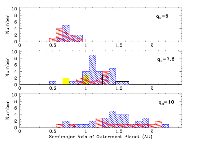
Figure 8: The distribution of the semimajor axis of the outermost final planet formed for binary star systems with $q_{B}$ = 5 AU (top panel), $q_{B}$ = 7.5 AU (middle panel), and $q_{B}$ = 10 AU (bottom panel). The red bars represent simulations from Set A with $M_{\star}$ = $M_{C}$ = 0.5 M_⊙, whereas the blue bars represent systems from Set B with $M_{\star}$ = $M_{C}$ = 1.0 M_⊙. Also shown in the middle panel are the results from Set C in which $M_{\star}$ = 0.5 M_⊙ and $M_{C}$ = 1.0 M_⊙ (solid yellow bars), and from Set D with $M_{\star}$ = 1.0 M_⊙ and $M_{C}$ = 0.5 M_⊙ (solid black line). Although the semimajor axes extend to larger values in binary systems with larger periastron, the inner edge of the distribution is roughly determined by the inner edge of the initial disk of embryos, as in the single star case, i.e., the presence of different stellar companions has a minimal effect on the inner terrestrial region.

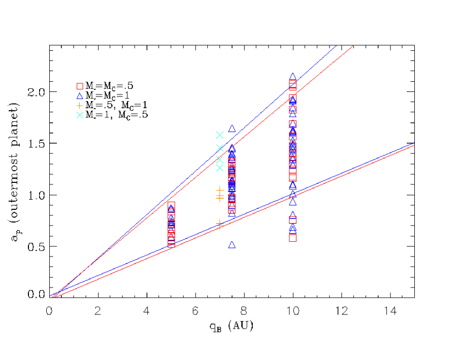
Figure 9: The semimajor axis of the outermost final planet formed in each simulation as a function of binary periastron, $q_{B}$. The red square symbols represent binary systems with $M_{\star}$ = $M_{C}$ = 0.5 M_⊙ (Set A), while the blue triangle symbols represent systems with $M_{\star}$ = $M_{C}$ = 1.0 M_⊙ (Set B). A fit to the (2$\sigma$) standard deviation for both Sets A and B are also shown in red and in blue. The values from Set C (where $\mu$ = 2/3) are shown with orange plus symbols, and those from Set D ($\mu$ = 1/3) are displayed with light blue X symbols. Note that the symbols from Sets C and D have been offset by –0.5 AU for clarity. The expectation value, and also the width of each distribution, grow in a nearly linear fashion with increasing values of binary periastron $q_{B}$.

The semimajor axis of the outermost planet can be used as a measure of the size of the terrestial planet system. Figure 8 shows the distribution of the semimajor axis of the outermost final planet, $a_{p_{max}}$, formed in each simulation for systems with $q_{B}$ = 5 AU (top panel), 7.5 AU, (middle panel), and 10 AU (lower panel). Note that twice as many integrations have been performed in Set B than in Set A. Figure 8 shows a clear trend: as the binary periastron increases, the distribution of semimajor axes of the outermost planet becomes wider and its expectation value shifts to larger values. This trend of a larger distribution in semimajor axis for increasing $q_{B}$ is also demonstrated in Figure 9, for which the outermost semimajor axis of the final planets is plotted directly as a function of $q_{B}$. Both the expectation value and the width of each distribution clearly grow (in a nearly linear fashion) with increasing values of binary periastron $q_{B}$.

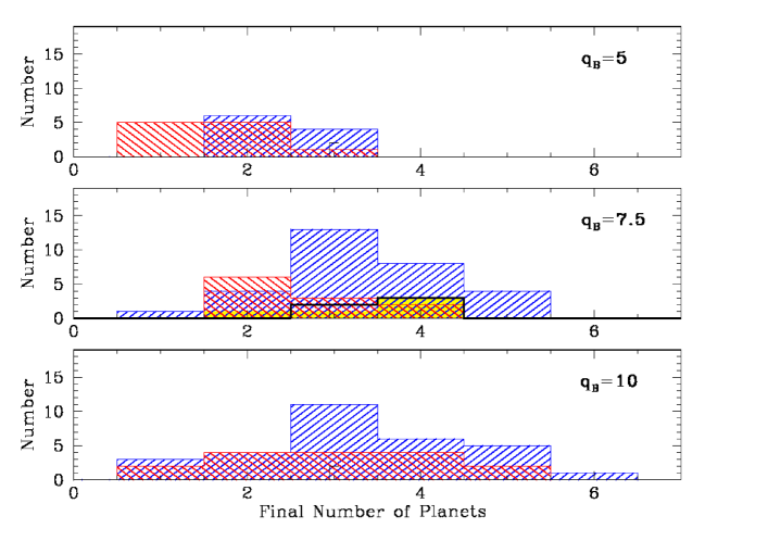
Figure 10: Histograms of the number of final planets formed for binary star systems with $q_{B}$ = 5 AU (top panel), $q_{B}$ = 7.5 AU (middle panel), and $q_{B}$ = 10 AU (bottom panel). The colors correspond to the different sets of runs as described in Figure 8. The typical number of final planets clearly increases in systems with larger stellar periastron, and also when the companion star is less massive than the primary (for a given stellar mass ratio).

The distributions of the total number of final planets formed are shown in Figure 10 for simulations with $q_{B}$ = 5 AU (top panel), 7.5 AU, (middle panel), and 10 AU (lower panel). In general, a smaller binary periastron results in a larger percentage of mass loss, and a smaller number of final planets. From 1 – 3 planets formed in all systems with $q_{B}$ = 5 AU, 1 – 5 planets remained in systems with $q_{B}$ = 7.5 AU, and 1 – 6 planets formed in all systems with $q_{B}$ = 10 AU. The range in the number of possible planets thus grows with increasing binary periastron; similarly, the average number of planets formed in the simulations is an increasing function of $q_{B}$. In the $q_{B}$ = 7.5 AU set with equal mass stars of 1 M_⊙, shown in blue, an average of 2.8 planets formed in the distribution of our largest set of 30 integrations. The distribution extends farther out if the perturbing star is smaller relative to the central star for a given stellar mass ratio, and slightly farther out when the stars are more massive relative to the disk.

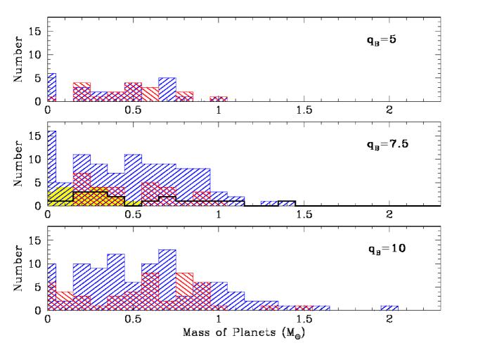
Figure 11: Histograms of the final masses of planets formed within binary star systems with $q_{B}$ = 5 AU (top panel), $q_{B}$ = 7.5 AU (middle panel), and $q_{B}$ = 10 AU (bottom panel). The colors correspond to the different sets of runs as described in Figure 8. Although the size of the stable region shrinks as $q_{B}$ gets smaller, the median mass of the final planets does not vary greatly for a given $q_{B}$, suggesting that planet formation remains efficient in the stable regions.

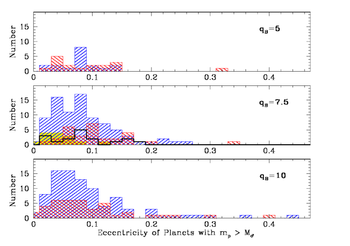
Figure 12: Distributions of the eccentricities of final planets that are more massive than Mars are shown for systems with $q_{B}$ = 5 AU (top panel), $q_{B}$ = 7.5 AU (middle panel), and $q_{B}$ = 10 AU (bottom panel). The colors correspond to different sets of runs as described in Figure 8. The majority of planets orbit on nearly circular ($e\lesssim$ 0.1) orbits despite the proximity of the stellar companion.

Figure 11 shows the distribution of final planetary masses (in units of the Earth’s mass, M_⊕) formed in systems with $q_{B}$ = 5 AU (top panel), 7.5 AU, (middle panel), and 10 AU (lower panel). The median mass of the final planets doesn’t depend greatly on $q_{B}$. This result suggests that planet formation remains quite efficient in the stable regions, but that the size of the stable region shrinks as $q_{B}$ gets smaller. This trend is consistent with the decline in the number of planets seen in Figure 10. When the periastron value becomes as small as 5 AU, planets only form within 1 AU, and the mass distribution tilts toward $m_{p}<M_{\oplus}$, i.e., the formation of Earth-like planets is compromised. Figure 12 displays the distribution of eccentricities for the planets that are more massive than the planet Mars that remain in systems with $q_{B}$ = 5 AU (top panel), $q_{B}$ = 7.5 AU (middle panel), and $q_{B}$ = 10 AU (bottom panel). The distribution of eccentricities reaches relatively high values in several simulations (up to $\sim$ 0.45 in the system with the largest periastron). However, the majority of planets orbit on nearly circular ($e\lesssim$ 0.1) orbits.

5 Conclusions

This paper studies the late stages of terrestrial planet formation in binary star systems. These dynamical systems – disks of planetesimals orbiting in the potential of a binary star – are chaotic and display extremely sensitive dependence on their initial conditions. In the present context, as for analogous models of terrestrial planet formation around a single star (Chambers et al. 2002, Quintana & Lissauer 2006), if one of the planetesimals is moved only one meter forward along its initial orbit, the difference in the final number, masses, and/or orbits of terrestrial planets that form can be substantial (see Figure 1). Effectively equivalent starting states thus lead to different final states. As a result, the numerical simulation of accretion from any particular initial configuration cannot be described in terms of a single outcome, but rather must be considered as a distribution of outcomes. To account for this complication, we performed multiple realizations with effectively equivalent starting conditions for all of the binary systems considered herein. Fortunately, even though the systems are chaotic and do not have a single outcome, the distributions of outcomes are well-defined. Further, these distributions show clear trends with varying properties of the binary star systems and can be used to study the effects of binaries on the planet formation process.

Our exploration of parameter space shows how binary orbital parameters affect terrestrial planet formation. We find that the presence of a binary companion of order 10 AU away acts to limit the number of terrestrial planets formed and the spatial extent of the terrestrial planet region, as shown by Figures 3 – 12. To leading order, the periastron value $q_{B}$ is the most important parameter in determining binary effects on planetary outcomes (more predictive than $a_{B}$ or $e_{B}$ alone). In our ensemble of 108 wide binary simulations that began with equal mass stars, from 1 – 6 planets formed with semimajor axes $\lesssim$ 2.2 AU of the central star in binary systems with $q_{B}$ = 10 AU, from 1 – 5 planets formed within 1.7 AU for systems with $q_{B}$ = 7.5 AU, and from 1 – 3 planets formed within 0.9 AU when $q_{B}$ = 5 AU. Nonetheless, for a given binary perisatron $q_{B}$, fewer planets tend to form in binary systems with larger values of ($a_{B}$, $e_{B}$) (see Figure 4).

Binary companions also limit the extent of the terrestrial planet region in nascent solar systems. As shown in Figures 3, 5, and 7 – 9, wider binaries allow for spatially larger systems of terrestrial planets. Once again, binary periastron is the most important variable in determining the extent of the final system of terrestrial planets (as measured by the semimajor axis of the outermost planet). However, for a given periastron, the sizes of the terrestrial planet systems show a wide distribution. In these simulations, the initial disk of planetesimals extends out to 2 AU, so we do not expect terrestrial planets to form much beyond this radius. For binary periastron $q_{B}$ = 10 AU, the semimajor axis of the outermost planet typically lies near 2 AU, i.e., the system explores the entire available parameter space for planet formation. Since these results were obtained with equal mass stars (including those with $M$ = 1.0 M_⊙), we conclude that the constraint $q_{B}\gtrsim 10$ AU is sufficient for binaries to leave terrestrial planet systems unperturbed. With smaller binary periastron values, the resulting extent of the terrestrial planet region is diminished. When binary periastron decreases to 5 AU, the typical system extends only out to $a_{p}\sim$ 0.75 AU and no system has a planet with semimajor axis beyond 0.9 AU (but note that we did not perform simulations with $q_{B}=$ 5 AU and small $e_{B}$).

While the number of forming planets and their range of orbits is restricted by binary companions, the masses and eccentricities of those planets are much less affected. Both Figures 7 and 12 suggest that planet eccentricities tend to arise from the same distribution (with a broad peak near $e_{P}=0.08$ and a tail toward higher values) for all of the systems considered in this study. The distribution of planet masses is nearly independent of binary periastron (see Figure 11), although the wider binaries allow for a few slightly more massive terrestrial planets to form. Finally, we note that the time scales required for terrestrial planet formation in these systems lie in the range 50 – 200 Myr, consistent with previous findings (e.g., Chambers 2001, Quintana et al. 2002, Quintana & Lissauer 2006), and largely independent of the binary properties. This result is not unexpected, as the clock for the accumulation of planetesimals is set by their orbit time and masses (Safranov 1969), and not by the binary orbital period.

Whitmire et al. (1998) have analyzed the effects of perturbations by a binary companion on planetesimals during the earlier stages of planetary growth. Assuming that collisions at velocities $>$ 100 m/s disrupt planetesimals, they find that if two 1 M_⊙ stars have periastron $q_{B}<$ 16 AU, then planetary growth at 1 AU is inhibited. This criterion is more limiting than the results of this paper suggest. But note that Whitmire et al.’s model does not include gas. Perturbations by a gaseous disk can align planetesimal orbits, reducing collision velocities and thereby allowing growth to proceed and produce bodies of the sizes that we use as initial conditions over a larger range of semimajor axis (Kortenkamp & Wetherill 2000).

Our work has important implications regarding the question of what fraction of stars might harbor terrestrial planetary systems. The majority of solar-type stars live in binary systems, and binary companions can disrupt both the formation of terrestrial planets and their long term prospects for stability. Approximately half of the known binary systems are wide enough (in this context, having sufficiently large values of periastron) so that Earth-like planets can remain stable over the entire 4.6 Gyr age of our Solar System (David et al. 2003, Fatuzzo et al. 2006). For the system to be stable out to the distance of Mars’s orbit, the binary periastron $q_{B}$ must be greater than about 7 AU, and about half of the observed binaries have $q_{B}>7$ AU. Our work on the formation of terrestrial planets shows similar trends. When the periastron of the binary is larger than about $q_{B}$ = 10 AU, even for the case of equal mass stars, terrestrial planets can form over essentially the entire range of orbits allowed for single stars (out to the edge of the initial planetessimal disk at 2 AU). When periastron $q_{B}<10$ AU, however, the distributions of planetary orbital parameters are strongly affected by the presence of the binary companion (see Figures 7 – 12). Specifically, the number of terrestrial planets and the spatial extent of the terrestrial planet region both decrease with decreasing binary periastron. When the periastron value becomes as small as 5 AU, planets no longer form with $a=1$ AU orbits and the mass distribution tilts toward $m_{p}<$ 1 M_⊕, i.e., the formation of Earth-like planets is compromised. Note that the results from our simulations can be scaled for different star and disk parameters with the formulae presented in Appendix C of Quintana & Lissauer (2006). Given the enormous range of orbital parameter space sampled by known binary systems, from contact binaries to separations of nearly a parsec, the range of periastron where terrestrial planet formation is affected is quite similar to the range of periastron where the stability of Earth-like planets is compromised. As a result, about 40 – 50% of binaries are wide enough to allow both the formation and the long term stability of Earth-like planets in S-type orbits encircling one of the stars. Furthermore, approximately 10% of main sequence binaries are close enough to allow the formation and long-term stability of terrestrial planets in P-type circumbinary orbits (David et al. 2003, Quintana & Lissauer 2006). Given that the galaxy contains more than 100 billion star systems, and that roughly half remain viable for the formation and maintenence of Earth-like planets, a large number of systems remain habitable based on the dynamic considerations of this research.

Table 1: The Outermost Stable S-type Orbit ($a_{c}$)

$e_{B}$			$\mu$=1/3		$\mu$=1/2		$\mu$=2/3
0			-		0.26		-
0.25			0.23		0.20		0.11
0.5			-		0.12		-
0.625			-		0.08		-
0.75			-		0.06		-
0.8125			-		0.04		-
0.875			-		0.03		-

Table 2: Binary Star Parameters

		$q_{B}$ (AU)	$a_{B}$ (AU)	$e_{B}$	$a_{c}$ (AU)	# Runs
Set A⋆		5	10	0.5	1.2	5
		5	20	0.75	1.2	3
		5	40	0.875	1.2	3
		7.5	10	0.25	2	5
		7.5	20	0.625	1.6	3
		7.5	40	0.8125	1.6	3
		10	10	0	2.6	5
		10	13$\frac{1}{3}$	0.25	2.6	3
		10	20	0.5	2.4	3
		10	40	0.75	2.4	5
Set B		5	10	0.5	1.2	10
		7.5	10	0.25	2	30
		10	10	0	2.6	10
		10	40	0.75	2.4	20
Set C		7.5	10	0.25	1.1	5
Set D		7.5	10	0.25	2.3	5

Table 3: Statistics for Final Planetary Systems

$\bf System$	# Runs	$N_{p}$	$N_{m}$	$a_{p_{max}}$	$a_{p_{max}}$/$a_{c}$	$Q_{p}$	$Q_{p}$/$q_{B}$	$S_{m}$	$m_{l_{\star}}$	$m_{l_{\infty}}$	$E/E_{0}$	$L/L_{0}$
A_10_.5	5	2	0.2	0.90	0.65	0.95	0.17	0.66	34.9	31.5	1.64	0.74
A_20_.75	3	1.3	0	0.71	0.68	0.52	0.13	0.93	40.4	31.3	1.76	0.71
A_40_.875	3	1	0	0.60	0.47	0.52	0.13	1.00	42.9	34.4	1.86	0.67
A_10_.25	5	3.2	0	1.32	0.59	1.43	0.17	0.50	9.6	39.8	1.49	0.79
A_20_.625	3	2.3	0	1.32	0.79	1.24	0.18	0.68	38.9	8.8	1.43	0.81
A_40_.8125	3	1.7	0.3	0.97	0.58	0.85	0.14	0.64	34.2	18.1	1.52	0.78
A_10_0	5	3.2	1.2	2.07	0.77	2.50	0.23	0.50	0.2	39.5	1.39	0.84
A_13.3_.25	3	3	0.3	1.68	0.50	1.50	0.14	0.41	5.36	27.0	1.31	0.85
A_20_.5	3	2.3	0	1.56	0.59	1.39	0.16	0.52	30.8	1.7	1.31	0.87
A_40_.75	5	1.8	0	1.47	0.45	2.06	0.13	0.68	26.4	12.4	1.44	0.81
B_10_.5	10	1.8	0.6	0.87	0.62	0.99	0.16	0.73	35.5	29.2	1.62	0.74
B_10_.25	30	2.8	0.5	1.65	0.58	1.81	0.17	0.56	9.8	30.1	1.36	0.83
B_10_0	10	3.8	0.7	2.15	0.64	2.78	0.18	0.47	0.0	25.7	1.22	0.90
B_40_.75	20	2.6	0.2	1.85	0.55	1.99	0.15	0.60	19.2	7.5	1.26	0.87
C_10_.25_2/3	5	2.8	0.6	1.05	0.81	1.06	0.12	0.53	0.0	72.4	1.66	0.74
D_10_.25_1/3	5	3.4	0.2	1.58	0.61	1.79	0.21	0.54	25.5	0.3	1.24	0.88
MVEM	$\cdots$	4.0	0.0		$\cdots$		$\cdots$	0.51	$\cdots$	$\cdots$	$\cdots$	$\cdots$
SJS	31	3.0	0.7		$\cdots$		$\cdots$	0.51	23.9	2.0	1.26	0.87
Sun	3	4.3	12		$\cdots$		$\cdots$	0.39	0.0	0.5	1.06	1.01
Sun ($a<$ 2 AU)	3	3.0	0.7		$\cdots$		$\cdots$	0.48	0.0	18.7‡	1.21	0.90
$\alpha$ Cen A ($i$ = 0∘)	4	4.3	0		$\cdots$		$\cdots$	0.40	11.6	0.8	1.12	0.94

References

- Butler et al. (2006) Butler, R. P., Wright, J. T., Marcy, G. W., Fischer, D. A., Vogt, S. S., Tinney, C. G., Jones, H. R. A., Carter, B. D., Johnson, J. A., McCarthy, C., & Penny, A. J. 2006, ApJ, 646, 505
- Chambers (2001) Chambers, J. E. 2001, Icarus, 152, 205
- Chambers et al. (2002) Chambers, J. E., Quintana, E. V., Duncan, M. J., & Lissauer, J. J. 2002, AJ, 123, 2884
- David et al. (2003) David, E., Quintana, E. V., Fatuzzo, M., & Adams, F. C. 2003, PASP, 115, 825
- Duquennoy and Mayor (1991) Duquennoy, A., & Mayor, M. 1991, A&A, 248, 485
- Eggenberger et al. (2004) Eggenberger, A., Udry, S., & Mayor, M. 2004, A&A, 417, 353
- Fatuzzo et al. (2006) Fatuzzo, M., Adams, F. C., Gauvin, R., & Proszkow, E. M. 2006, PASP, In press.
- Hatzes et al. (2003) Hatzes, A. P., Cochran, W. D., Endl, M., McArthur, B., Paulson, D. B., Walker, G. A. H., Campbell, B., & Yang, S. 2003, ApJ, 599, 1383
- Holman & Wiegert (1999) Holman, M. J. & Wiegert, P. A. 1999, AJ, 117, 621
- Kasting et al. (1993) Kasting, J. F., Whitmire, D. P., & Reynolds, R. T. 1993, Icarus, 101, 108
- Konacki (2005) Konacki, M. 2005, Nature, 436, 230
- Kortenkamp & Wetherill (2000) Kortenkamp, S. J. & Wetherill, G. W. 2000, Icarus, 143, 60
- Lissauer et al. (2004) Lissauer, J. J., Quintana, E. V., Chambers, J. E., Duncan, M. J., & Adams, F. C. 2004, RevMexAA, 22, 99
- Marzari and Scholl (2000) Marzari, F., & Scholl, H. 2000, ApJ, 543, 328
- Nelson (2003) Nelson, R. P. 2003, MNRAS 345, 233
- Nelson and Papaloizou (2003) Nelson, R. P. & Papaloizou, J. C. B. 2003, in Proceedings of the Conference on Towards Other Earths, DARWIN/TPF and the Search for Extrasolar Terrestrial Planets, ed. Fridlund, M., & Henning, T. (Noordwijk: ESA Publications Division ESA SP-539), 175
- Pichardo et al. (2005) Pichardo, B., Sparke, L. S., & Aguilar, L. A. 2005, MNRAS, 359, 521
- Queloz et al. (2000) Queloz, D., Mayor, M., Weber, L., Blecha, A., Burnet, M., Confino, B., Naef, D., Pepe, F., Santos, N., & Udry, S. 2000, A&A, 354, 99
- Quintana (2003) Quintana, E. V. 2003, in ASP Conf. Ser. 294, Scientific Frontiers in Research on Extrasolar Planets, ed. Deming, D., & Seager, S. (San Francisco: ASP), 319
- Quintana (2004) Quintana, E. V. 2004, Planet Formation in Binary Star Systems, Thesis (Ph.D.), University of Michigan, Ann Arbor (Ann Arbor: UMI Company)
- Quintana et al. (2002) Quintana, E. V., Lissauer, J. J., Chambers, J. E., & Duncan, M. J. 2002, ApJ, 576, 982
- Quintana & Lissauer (2006) Quintana, E. V., & Lissauer, J. J. 2006, Icarus, 185, 1
- Raghavan et al. (2006) Raghavan, D., Henry, T. J., Mason, B. D., Subasavage, J. P., Jao, W.-C., Beaulieu, T. D., & Hambly, N. C. 2006, ApJ, 646, 523
- Raymond et al. (2004) Raymond, S. N., Quinn, T., & Lunine, J. I. 2004, Icarus, 168, 1
- Saha et al. (1997) Saha, P., Stadel, J., & Tremaine, S. 1997, ApJ, 114, 409
- Turrini et al. (2005) Turrini, D., Barbieri, B., Marzari, F., Thebault, P., & Tricarico, P. 2005, MSAIS, 6, 172
- Whitmire et al. (1998) Whitmire, D. P., Matese, J. J., Criswell, L., & Mikkola, S. 1998, Icarus, 132, 196
- Wiegert & Holman (1997) Wiegert, P. A., & Holman, M. J. 1997, AJ, 113, 1445
- Wisdom & Holman (1991) Wisdom J., & Holman, M. 1991, AJ, 102, 1528
- Zucker et al. (2004) Zucker, S., Mazeh, T., Santos, N. C., Udry, S., & Mayor, M. 2004, A&A, 426, 695