Radio Emission Physics in the Crab Pulsar

Abstract

Our high time resolution observations of individual giant pulses in the Crab pulsar show that both the time and frequency signatures of the interpulse are distinctly different from those of the main pulse. Giant main pulses can occasionally be resolved into short-lived, relatively narrow-band nanoshots. We believe these nanoshots are produced by soliton collapse in strong plasma turbulence. Giant interpulses are very different. Their dynamic spectrum contains narrow, microsecond-long emission bands. We have detected these proportionately spaced bands from 4.5 to 10.5 GHz. The bands cannot easily be explained by any current theory of pulsar radio emission; we speculate on possible new models.

1 Introduction

What is the pulsar radio emission mechanism? Does the same mechanism always operate? Three types of models have been proposed to explain the radio emission: coherent charge bunches, plasma masers and strong plasma turbulence (e.g., Hankins et al. 2003, “HKWE”). Because each model makes different predictions for the time signature of the emission, our group has carried out ultra-high time resolution observations in order to compare the observed time signatures to those predicted by the models.

We have focused on the Crab nebula pulsar, because its occasional, very strong giant pulses are ideal targets for our observations. The dominant features of this star’s mean profile are a main pulse (MP) and an interpulse (IP). Although the relative amplitudes and detailed profiles of these features change with frequency, they can be identified from low radio frequencies ($\>\hbox{\lower 2.5pt\hbox{$\buildrel<\over{\sim}$}}\>300$ MHz) up to the optical and hard X-ray bands (Moffet & Hankins 1996). Some models suggest that the MP and IP come from low altitudes, above the star’s two magnetic poles. Other models suggest they come from higher altitudes, possibly relativistic caustics (Dyks et al. 2004) which connect to the two poles. In either case, the physical conditions in the emission region should be similar, and one would expect the same radio emission mechanism to be active in the IP and the MP. We were surprised, therefore, to find that the IP and MP have very different properties. It seems likely that they differ in their emission mechanisms, their propagation within the magnetosphere, or both.

2 Giant main pulses: strong plasma turbulence

We initially studied the MP at nanosecond time resolution, because it is usually brighter, and because giant pulses are more common at the rotation phase of the MP (Cordes et al. 2004). We found that most giant main pulses (GMPs) consist of one to several “microbursts”, each lasting a few microseconds at 5 GHz (HKWE). We recently extended our observations to higher frequencies, where 2 GHz of bandwidth is available at Arecibo. We found the temporal structure of GMPs is the same at higher frequencies, although the microburst duration is typically shorter than at 5 GHz. Figure 1 shows a typical example. The dynamic spectrum of the microbursts turns out to be broadband, filling our entire observing bandwidth. An occasional MP, however, contains much shorter, relatively narrow-band, “nanoshots” (HKWE; also Figures 2 and 3). Most of the time the nanoshots overlap, which is consistent with previous modelling of pulsar emission as amplitude-modulated noise; but in sparse GMPs the nanoshots can sometimes be individually resolved.

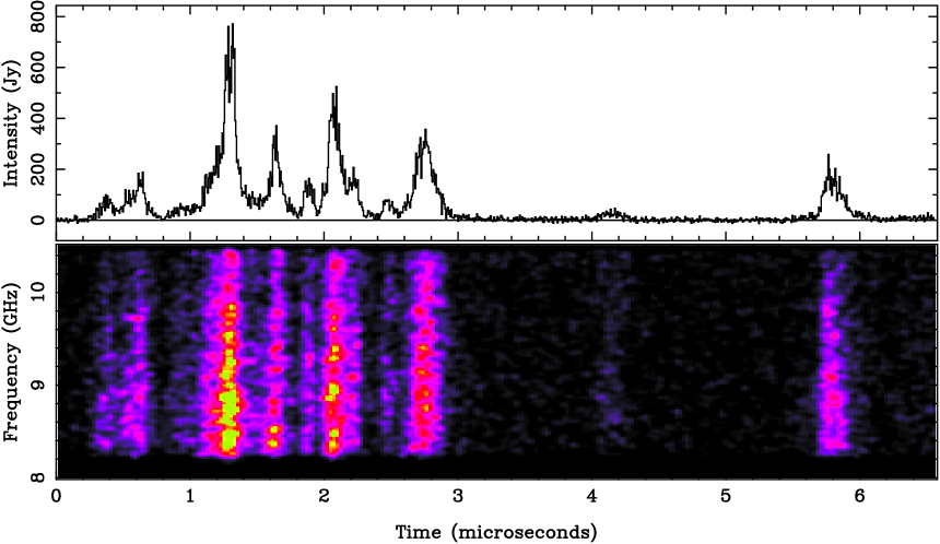
Figure 1: Total intensity and dynamic spectrum of a giant main pulse, observed at Arecibo and coherently dedispersed. As is typical of most GMPs, it contains several broad-band microbursts. The total intensity is plotted with 6.4-ns time resolution; the dynamic spectrum has 25.6-ns time resolution and 19.5-MHz frequency resolution.

We used simple scaling arguments, and numerical simulations from Weatherall (1998), to compare the nanoshots to predictions of the three competing theoretical models of the radio emission mechanisms. The time signature of the nanoshots disagrees with predictions of the maser and charge bunching models; but both the time and frequency signatures are consistent with Weatherall’s numerical models of plasma emission by soliton collapse in strong plasma turbulence. His models predict nanoshot durations at frequency $\nu$ to be $\nu\delta t\sim O(10)$; an individual nanoshot is relatively narrow-band, $\delta\nu/\nu\sim O(0.1)$. In HKWE we suggested, based on the time signature of the nanoshots, that strong plasma turbulence is the emission mechanism in GMPs. The time and spectral signatures of the nanoshots in our recent high-frequency work are also consistent with these models. We thus propose that microbursts in giant main pulses are collections of nanoshots, produced by strong plasma turbulence in the emission region.

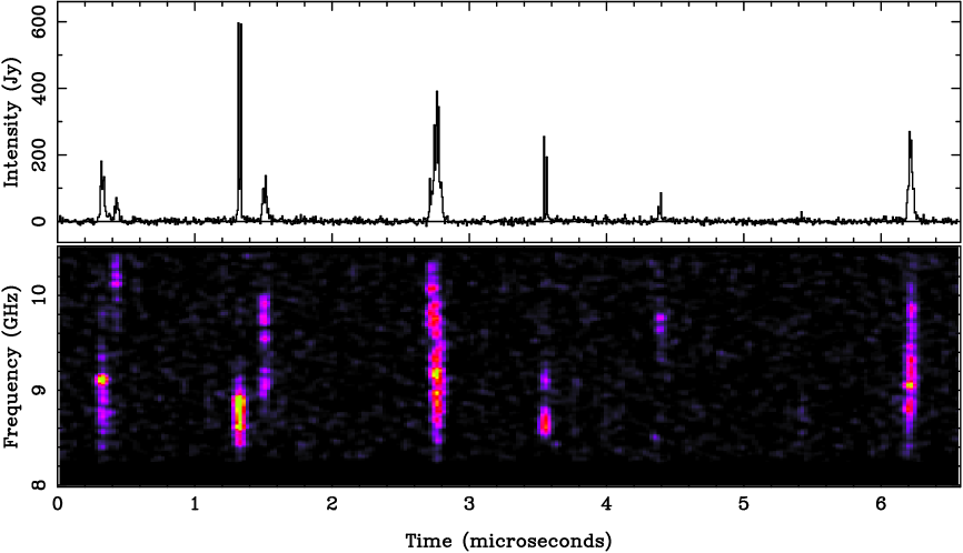
Figure 2: Another giant main pulse, processed and displayed the same as in Figure 1, in which the microbursts are sparse and short-lived. At higher time resolution some of these bursts can be resolved into even shorter nanoshots, as in Figure 3. Note the relatively narrow-band nature of individual nanoshots. We infer that the longer-duration, broad-band microbursts, such as those in Figure 1, are “clouds” of these nanoshots.

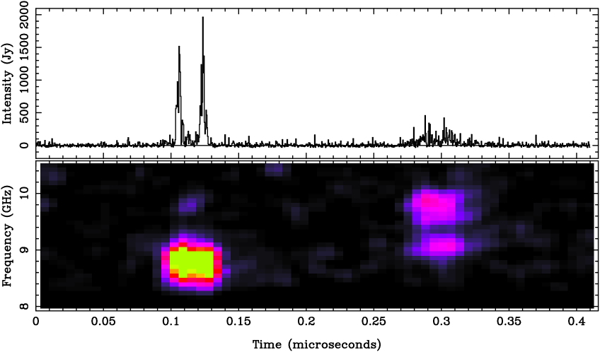
Figure 3: A short portion of the sparse main pulse shown in Figure 2, with total intensity displayed at our maximum time resolution, 0.4 ns. This reveals the temporal signature of individual nanoshots. We believe the nanoshots are created by collapse of solitons in strong plasma turbulence. The dynamic spectral resolution is 78 MHz and 6.4 ns.

If our suggestion is correct, it has one important consequence. Plasma flow in the radio emission region should be highly dynamic. The plasma flow will be smooth only if the local charge density is exactly the Goldreich-Julian (GJ) value, so that the rotation-induced electric field, $\mathbf{E}$, is fully shielded. Because plasma turbulent emission is centered on the comoving plasma frequency ($\nu_{p}\propto\sqrt{\gamma_{b}n}$, for number density $n$ and bulk Lorentz factor $\gamma_{b}$), we can determine the local density in the radio emission region (cf. also Kunzl et al. 1998). We find that low radio frequencies come from densities too low to match the GJ value anywhere in the magnetosphere. Because the emitting plasma feels an unshielded $\mathbf{E}$ field, and feeds back on that field as its charge density fluctuates, we expect unsteady plasma flow (and consequently unsteady radio emission).

3 Giant interpulses: emission bands

In order to test our hypothesis that strong plasma turbulence governs the emission physics in the Crab pulsar, we went to higher frequencies to get a larger bandwidth and shorter time resolution. In addition to the MP, we observed giant pulses from the IP, because at high frequencies giant pulses are more common at the rotation phase of the IP. When we used the method described in HWKE to observe giant interpulses (GIPs) with a broad bandwidth, from 6-8 or 8-10 GHz, we were astonished to find that GIPs have very different properties from giant main pulses. GIPs differ from GMPs in time signature, polarization, dispersion and spectral properties. In this paper we summarize our new results; we will present more details in a forthcoming paper (Hankins & Eilek 2007).

3.1 Emission bands in the interpulse

The most striking difference between the IP and the MP is found in the dynamic spectrum. A giant IP contains microsecond-long trains of emission bands, as illustrated in Figures 4 and 5. The bands are grouped into regular “sets”; 2 or 3 band sets can usually be identified in a given IP. Individual band sets last a few $\mu$s. In some pulses new band sets turn on partway through the pulse, often coincident with a secondary burst of total intensity. Every giant interpulse we recorded between 4.5 and 10.5 GHz, during 20 observing days from 2004 to 2006, displays these emission bands. However, giant main pulses observed at the same time and processed identically do not show the bands. The bands are, therefore, not due to instrumental or interstellar effects, but are intrinsic to the star.

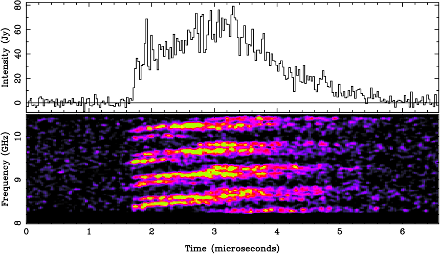
Figure 4: A giant interpulse from the Crab pulsar, observed and processed in exactly the same way as the main pulses in Figures 1 through 3. Total intensity time resolution 25.6 ns; dynamic spectral resolution 19.5 MHz and 25.6 ns. The banded frequency structure in the dynamic spectrum occurs in every IP we have recorded above 5 GHz. In this example, two band sets can be identified, starting at 1 $\mu$s, each containing four bright bands; a third band set starts near 2 $\mu$s. Note the apparent drift to higher frequencies for each band set.

At first glance the bands appear to be uniformly spaced. However, closer inspection of our data shows that the bands are proportionally spaced. The spacing between two adjacent bands, at $\nu_{1}$ and $\nu_{2}$, depends on the mean frequency, as $\Delta\nu/\nu=2(\nu_{2}-\nu_{1})/(\nu_{2}+\nu_{1})\simeq 0.06$. Thus, two bands near 6 GHz are spaced by $\sim 360$ MHz; two bands near 10 GHz are spaced by $\sim 600$ MHz. This proportional spacing is robust; a set of emission bands can drift in frequency (usually upwards, as in Figures 3 and 4), but their frequency spacing stays constant. All bands in a particular set appear almost simultaneously, to within $\sim 0.1\mu$s; they must all come from a region no larger than $\sim 30$ m across.

We suspect the bands extend over at least a $5\!-\!6$ GHz range in a single GIP, but do not occur below $\sim 4$ GHz. While we have not been able to observe more than 2 GHz simultaneously, we have seen no evidence that a given band set cuts off within our observable bandwidth. The characteristics of the bands (proportional spacing, duration, onset relative to total intensity microbursts) are unchanged from 5 to 10 GHz. In addition, the rotation phase of the high-frequency IP is slightly shifted relative to the low-frequency IP (Moffett & Hankins 1996). This phase offset suggests that the bands do not continue to frequencies below $\sim 4$GHz.

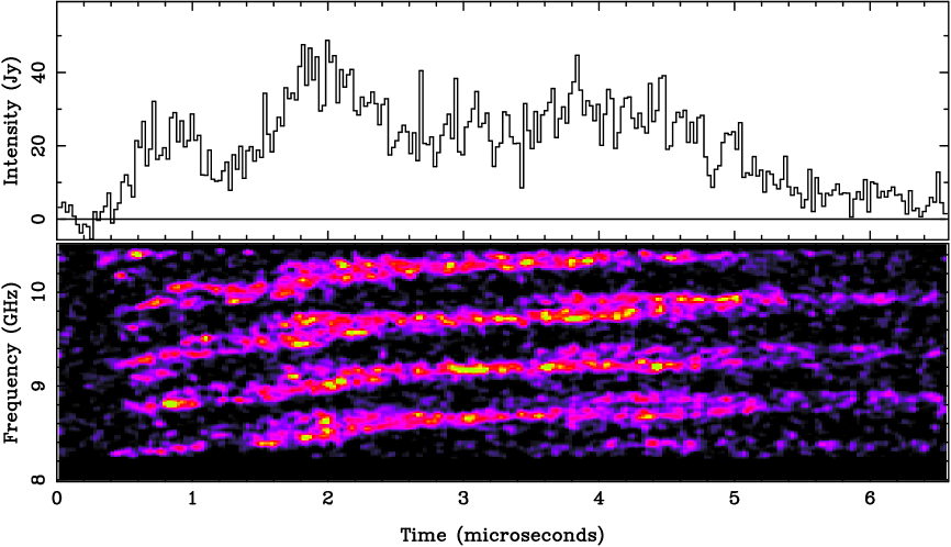
Figure 5: Another giant interpulse, observed on the same day as the IP in Figure 4 and processed and displayed in the same way. Four emission band sets can be identified, including a set which coincides with the second microburst near $2\,\mu$s, and another which coincides with a third microburst near $4\,\mu$s. This example also shows the characteristic band drift to higher frequencies.

3.2 Possible causes of the emission bands

The dynamic spectrum of the giant interpulses does not match any of the three types of emission models described above. Because each of the models predicts narrow-band emission at the plasma frequency, none of them can explain the dynamic spectrum of the IP. A new approach is required here, which may “push the envelope” of pulsar radio emission models.

While we remain perplexed by the dramatic dynamic spectrum of the interpulse, we are exploring possible models. This exercise is made particularly difficult by the fact that the emission bands are not regularly spaced. Because of this, models that initially seemed attractive must be rejected. As an example, if the emission bands were uniformly spaced they could be the spectral representation of a regular emission pulse train. Many authors have invoked regularly spaced plasma structures (sparks or filaments), whose passage across the line of sight could create such a pulse train. Alternatively, strong plasma waves with a characteristic frequency will also create a regular emission pulse train. The dynamic spectrum of either of these models would contain emission bands at constant spacing; the proportional spacing we observe disproves both of these hypotheses.

We have looked to solar physics for insight. We initially remembered split bands in the dynamic spectra of Type II solar flares, which are thought to be plasma emission from low and high density regions associated with a shock propagating through the solar corona. This does not seem to be helpful for the Crab pulsar emission bands, because the radio-loud plasma would have to contain 10 or 15 different density stratifications, which seems unlikely. However, “zebra bands” seen in Type IV solar flares may be germane. These are parallel, drifting, narrow emission bands seen in the dynamic spectra of Type IV flares. Band sets containing from a few up to $\sim 30$ bands have been reported, with fractional spacing $\Delta\nu/\nu\sim.01-.03$ (e.g., Chernov et al. 2005). While zebra bands have not yet been satisfactorily explained, two classes of models have been proposed, invoking either resonant plasma emission or geometrical effects. Can similar models explain the emission bands in the Crab pulsar?

Resonant cyclotron emission. One possibility is plasma emission at the cyclotron resonance, $\omega-k_{\parallel}v_{\parallel}-s\Omega_{o}/\gamma=0$ (where $\gamma$ is the particle Lorentz factor, $\Omega_{o}=eB/mc$, and $s$ is the integer harmonic number). Kazbegi et al. (1991) proposed that this resonance operates at high altitudes in the pulsar magnetosphere, and generates X mode waves which can escape the plasma directly. Alternatively, “double resonant” cyclotron emission at the plasma resonant frequency has been proposed for solar flares (e.g., Winglee & Dulk 1986). In solar conditions, this resonance generates O mode waves, which must mode convert in order to escape the plasma. The emission frequency in these models is determined by local conditions where the resonance is satisfied; the band separation is $\Delta\nu\simeq\Omega_{o}/2\pi\gamma$.

Resonant emission models face several challenges before they can be considered successful. The emission must occur at high altitudes, in order to bring the resonant (cyclotron) frequency down to the radio band. Close to the light cylinder, where $B\sim 3\times 10^{5}$G, particle energies $\gamma\sim 10^{3}\!-\!10^{4}$ are needed. In addition, such models must be developed with specific calculations which address the fundamental plasma modes as well as their stability, under conditions likely to exist at high altitudes in the pulsar’s magnetosphere. It is not clear how the specific, proportional band spacing can be explained; perhaps a local gradient in the magnetic field must be invoked.

Geometrical models. Alternatively, the striking regularity of the bands calls to mind a special geometry. If some mechanism splits the emission beam coherently, so that it interferes with itself, the bands could be interference fringes. For instance, a downwards beam which reflects off a high density region could return and interfere with its upwards counterpart on the way back up. Simple geometry suggests that fringes occur if the two paths differ in length by only $c/\Delta\nu\>\hbox{\lower 2.5pt\hbox{$\buildrel<\over{\sim}$}}\>1$m. Another geometrical possibility is that cavities form in the plasma and trap some of the emitted radiation, imposing a discrete frequency structure in the plasma (e.g., LaBelle et al. 2003 for solar zebra bands). The scales required here are also small; the cavity scale must be some multiple of the wavelength.

Geometrical models also face several obstacles before they can be considered successful. The basic geometry is a challenge: what long-lived plasma structures can lead to the necessary interference or wave trapping? In addition, the proportional band spacing must be explained, perhaps by a variable index of refraction in the interference or trapping region.

Geometrical models also need an underlying broad-band radiation source, with at least 5 GHz bandwidth, in order to produce the emission bands we observe. Because standard pulsar radio emission mechanisms lead to relatively narrow-band radiation, at the local plasma frequency, they seem unlikely to work here. A double layer might be the radiation source; charges accelerated within the layer should radiate broadband, up to $\nu\sim L/2\pi c$, if $L$ is the thickness of the acceleration region within the double layer. Once again this is a small-scale effect; emission at 10 GHz requires $L\sim 1$ cm.

4 Final thoughts

Our high time resolution observations of giant pulses from the Crab pulsar have raised as many questions as they have answered. The time and frequency signatures of giant main pulses are consistent with predictions of one current model of pulsar radio emission, namely, strong plasma turbulence. However, the time and frequency signatures of giant interpulses are totally different, and do not seem to match the predictions of any current model. This result is especially surprising because magnetospheric models generally ascribe the main pulse and the interpulse to physically similar regions, which simply happen to be on opposite sides of the star. One important clue may be the offset in rotation phase between the high-radio-frequency interpulse, and the interpulse which is seen at low radio frequencies and also in optical and X-ray bands. Does the high-frequency interpulse originate in an unexpected part of the star’s magnetosphere, where different physical conditions produce such different radiation signatures?

- [1] Chernov, G.P., Yan, Y.H., Fu, Q. J. & Tah, Ch.M., 2005, A&A, 437, 1047
- [2] Cordes, J.M., Bhat, N.D.R., Hankins, T.H., McLaughlin, M.A. & Kern, J., 2004, ApJ, 612, 375
- [3] Dyks, J., Harding, A.K. & Rudak, B., 2004, ApJ, 606, 1125
- [4] Hankins, T.H., Kern. J.S., Weatherall, J.C. & Eilek, J.A., 2003, Nature, 422, 141
- [5] Hankins, T.H. & Eilek, J.A., 2007, in preparation
- [6] Kazbegi, A.Z., Machabeli, G.Z. & Melikidze, G.I., 1991, MNRAS, 253, 377
- [7] Kunzl, T., Lesch, H., Jessner, A. & von Hoensbroech, A., 1998, ApJ, 505, L139
- [8] LaBelle, J., Treumann, R.A., Yoon, P.H. & Karlicky, M., 2003, ApJ, 593, 1195
- [9] Moffett, D.A. & Hankins, T. H., 1996, ApJ, 468, 779
- [10] Weatherall, J.C., 1998, ApJ, 506, 341
- [11] Winglee, R.M. & Dulk, G.A., 1986, ApJ, 307, 808