Polarisation of high-energy emission in a pulsar striped wind

Abstract

Recent observations of the polarisation of the optical pulses from the Crab pulsar motivated detailed comparative studies of the emission predicted by the polar cap, the outer gap and the two-pole caustics models.

In this work, we study the polarisation properties of the synchrotron emission emanating from the striped wind model. We use an explicit asymptotic solution for the large-scale field structure related to the oblique split monopole and valid for the case of an ultra-relativistic plasma. This is combined with a crude model for the emissivity of the striped wind and of the magnetic field within the dissipating stripes themselves. We calculate the polarisation properties of the high-energy pulsed emission and compare our results with optical observations of the Crab pulsar. The resulting radiation is linearly polarised. In the off-pulse region, the electric vector lies in the direction of the projection on the sky of the rotation axis of the pulsar, in good agreement with the data. Other properties such as a reduced degree of polarisation and a characteristic sweep of the polarisation angle within the pulses are also reproduced.

1 Introduction

The high-energy, pulsed emission from rotating magnetised neutron stars is usually explained in the framework of either the polar cap or the outer gap models. Although the existence of such gaps is plausible [(Pétri et al. 2002)], these models still suffer from the lack of a self-consistent solution for the pulsar magnetosphere. Nevertheless, recent observations of the polarisation of the optical pulses from the Crab [(Kanbach et al. 2003)] motivated detailed comparative studies of the emission predicted by the polar cap, the outer gap and the two-pole caustics models [(Dyks et al. 2004)]. In all of these models, the radiation is produced within the light cylinder. However, the pulse profile is determined by the assumed geometry of the magnetic field and the location of the gaps. None of these models is able to fit the optical polarisation properties of the Crab pulsar.

An alternative site for the production of pulsed radiation has been investigated [(Kirk et al. 2002)], based on the idea of a striped pulsar wind, originally introduced by [Coroniti (1990)] and [Michel (1994)]. Emission from the striped wind originates outside the light cylinder and relativistic beaming effects are responsible for the phase coherence of the synchrotron radiation. A strength of this model is that the geometry of the magnetic field, which is the key property determining the polarisation properties of the emission, is relatively well-known.

In this work, we use an explicit asymptotic solution for the large-scale field structure related to the oblique split monopole and valid for the case of an ultra-relativistic plasma [(Bogovalov 1999)]. This is combined with a crude model for the emissivity of the striped wind and of the magnetic field within the dissipating stripes themselves. We calculate the polarisation properties of the high-energy pulsed emission and compare our results with optical observations of the Crab pulsar.

2 Stokes parameters

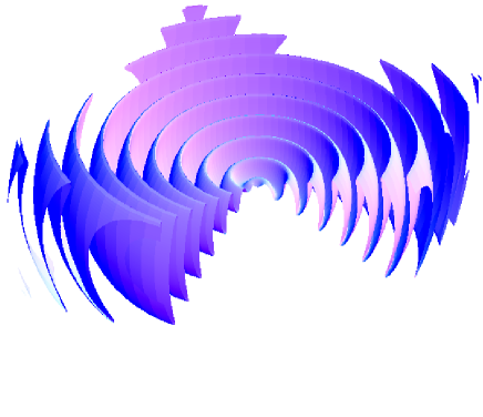
Figure 1: 3D structure of the current sheet in the striped wind. The rotating neutron star is located at the origin of the coordinate system.

Our magnetic field model is based on the asymptotic solution of the split monopole for the oblique rotator, valid for $r\gg r_{\rm L}$, and modified to take account of a finite width of the current sheet. We add a small meridional component in this sheet in order to prevent the magnetic field from becoming identically zero. The 3-dimensional geometry of the current sheet is shown in figure 1. In spherical polar coordinates $(r,\theta,\varphi)$ centered on the star and with axis along the rotation axis, the radial field is small and neglected, $B_{r}\sim B_{\rm L}\,r_{\rm L}^{2}/r^{2}$, while the other components are:

$$B_{\theta} = B_{\rm L}\,\frac{r_{\rm L}}{r}\,b_{1,2}\,\eta_{\theta}(\Delta_{\theta},r,\theta,\varphi,t)$$ (1)

$$B_{\varphi} = B_{\rm L}\,\frac{r_{\rm L}}{r}\,\eta_{\varphi}(\Delta_{\varphi},r,\theta,\varphi,t)$$ (2)

$$\eta_{\varphi}(\Delta_{\varphi},r,\theta,\varphi,t) = \tanh\left[\Delta_{\varphi}\,\left(\cos\theta\,\cos\alpha+\right.\right.$$

$$\left.\left.\sin\theta\,\sin\alpha\,\cos\left\{\varphi-\Omega_{*}\,\left(t-\frac{r}{v}\right)\right\}\right)\right]$$

$$\eta_{\theta}(\Delta_{\theta},r,\theta,\varphi,t) = \frac{1}{\Delta_{\theta}}\,\frac{\partial\eta_{\varphi}(\Delta_{\theta},r,\theta,\varphi,t)}{\partial\varphi}$$ (4)

Here, $B_{\rm L}$ is a fiducial magnetic field strength, $v$ is the (radial) speed of the wind, $\Omega_{*}=c/r_{\rm L}$ is the angular velocity of the pulsar, with $r_{\rm L}$ the radius of the light cylinder, $\alpha$ is the angle between the magnetic and rotation axes, $b_{1,2}$ are parameters controlling the magnitude of the meridional field in the two current sheets present in one wavelength, and $\Delta_{\theta,\varphi}$ are parameters quantifying the sheet thickness. The functional form of $B_{\varphi}$ is motivated by exact equilibria of the planar relativistic current sheet [(Kirk & Skjæraasen 2003)]. However, in these equilibria the $B_{\theta}$ component, which has an important influence on the polarisation sweeps, is arbitrary. The $B_{\theta}$ we adopt corresponds to a small circularly polarised component of the pulsar wind wave, such as is expected if the sheets are formed by the migration of particles within the wave, as described qualitatively by [Michel (1971)].

For the particle distribution, we adopt an isotropic electron/positron distribution given by

$$N(E,\vec{p},\vec{r},t)=K(\vec{r},t)\,E^{-p}$$ (5)

where $K(\vec{r},t)$ is related to the number density of emitting particles. The radial motion of the wind imposes an overall $1/r^{2}$ dependence on this quantity, which is further modulated because the energization occurs primarily in the current sheet. The precise value in each sheet is chosen to fit the observed intensity of each sub-pulse. In addition, a small dc component is added, giving the off-pulse intensity. For the emissivity, we use the standard expressions for incoherent synchrotron radiation of ultra-relativistic particles. We assume the emission commences when the wind crosses the surface $r=r_{0}\gg r_{\rm L}$.

The calculation of the Stokes parameters as measured in the observer frame involves simply integrating the emissivity over the wind. For an observer, at time $t_{\rm obs}$, they are given by the following integrals:

$$\left\{\begin{array}[]{c}I_{\omega}\\ Q_{\omega}\\ U_{\omega}\end{array}\right\}(t_{\rm obs}) = \!\!\!\int_{r_{0}}^{+\infty}\!\!\!\!\!\int_{0}^{\pi}\!\!\!\int_{0}^{2\,\pi}\!\!\!\!\!\!s_{0}(\vec{r},t_{\rm ret})\left\{\begin{array}[]{c}\frac{p+7/3}{p+1}\\ \cos\,(2\,\tilde{\chi})\\ \sin\,(2\,\tilde{\chi})\end{array}\right\}d^{3}\vec{r}$$ (12)

where the retarded time is given by $t_{\rm ret}=t_{\rm obs}+\vec{n}\cdot\vec{r}/c$ and $\vec{n}$ is a unit vector along the line of sight from the pulsar to the observer. In this approximation the circular polarisation vanishes: $V=0$. The function $s_{0}$ is defined by:

$$s_{0}(\vec{r},t) = \kappa\,K(\vec{r},t)\,\frac{\mathcal{D}^{\frac{p+3}{2}}}{\omega^{\frac{p-1}{2}}}\,\left(\frac{B}{\Gamma}\,\sqrt{1-(\mathcal{D}\,\vec{n}\cdot\vec{b})^{2}}\right)^{\frac{p+1}{2}}$$ (13)

where $\omega$ is the angular frequency of the emitted radiation, and $\kappa$ is a constant factor that depends only on the nature of the radiating particles (charge $q$ and mass $m$) and the power law index $p$ of their distribution:

$$\kappa = \frac{\sqrt{3}}{2\,\pi}\,\frac{1}{4}\,\Gamma_{\rm Eu}\left(\frac{3\,p+7}{12}\right)\,\Gamma_{\rm Eu}\left(\frac{3\,p-1}{12}\right)\,$$ (14)

$$\frac{|q|^{3}}{4\,\pi\,\varepsilon_{0}\,m\,c}\,\left(\frac{3\,|q|}{m^{3}\,c^{4}}\right)^{\frac{p-1}{2}}$$

with $\Gamma_{\rm Eu}$ the Euler gamma function and $\mathcal{D}$ the Doppler boosting factor $\mathcal{D}=1/\Gamma\,(1-\vec{\beta}\cdot\vec{n})$. The direction of the local magnetic field in the observer’s frame is given by the unit vector $\vec{b}$ and the simplifying assumption has been made that this field has no component in the direction of the plasma velocity: $\vec{b}\cdot\vec{\beta}=0$. (In this case the magnetic field transformation from the rest frame $\vec{B}^{\prime}$ to the observer frame $\vec{B}$ is just $\vec{B}^{\prime}=\vec{B}/\Gamma$ and, thus, its direction remains unchanged.) The angle $\tilde{\chi}$ measures the inclination of the local electric field with respect to the projection of the pulsar’s rotation axis on the plane of the sky as seen in the observer’s frame. The degree of linear polarisation is defined by

$$\Pi=\frac{\sqrt{Q^{2}+U^{2}}}{I}$$ (15)

The corresponding polarisation angle, defined as the position angle between the electric field vector at the observer and the projection of the pulsar’s rotation axis on the plane of the sky is

$$\chi=\frac{1}{2}\,\arctan\left(\frac{U}{Q}\right)$$ (16)

3 Results

The upper left panel of Fig. 2 shows the intensity (Stokes parameter $I$) computed using our smoothed profile with $\Delta_{\theta}=1$, $\Delta_{\varphi}=5$, $b_{1}=0.1$ and $b_{2}=0.08$ for each sub-pulse. The electron density is

$$K=\frac{1}{r^{2}\,(1-0.6\,\eta_{\theta})}\,\left[\left(\frac{r_{\rm L}\,B_{\rm L}}{r\,B}\right)^{(p+1)/2}+\varepsilon-1\right]$$ (17)

where the parameter $\varepsilon=0.05$ sets the minimum electron density between the current sheets (in normalized units). The denominator $(1-0.6\,\eta_{\theta})$ introduces an asymmetry in the relative pulse peak intensity. The variation of the magnetic field and the particle density along the line of sight, are shown in the bottom panels of Fig. 2.

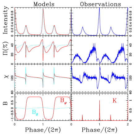
Figure 2: Light curve of intensity, degree of polarisation and position angle of the pulsed synchrotron emission obtained for our model and measurements of these quantities for the Crab pulsar. Models with Lorentz factor $\Gamma=20$ (solid red) and $50$ (dotted cyan) are shown. The bottom panels show the dependence on phase of the assumed magnetic field components and the particle density in the comoving frame.

The upper panels of Fig. 2 show the results of our computations on the left and the corresponding observed quantities [(Kanbach et al. 2003)] on the right. Comparison with the upper right-hand panel shows that the model reproduces the observed pulse profile quite accurately. In this example, we adopt an obliquity $\alpha=60\degr$ and an inclination of the rotation axis to the line of sight $\xi=\arccos(\vec{n}\cdot\vec{\Omega}_{*}/|\vec{\Omega}_{*}|)=60\degr$ and set the radius at which emission switches on to be $r_{0}=30r_{\rm L}$. The position angle of the projection of the pulsar’s rotation axis is set to $124\degr$ [(Ng & Romani 2004)]. The electron power law index $p=2$, as suggested by the relatively flat spectrum displayed by the pulsed emission between optical and gamma-ray frequencies [(Kanbach 1998)]. Results are shown for two values of the Lorentz factor of the wind: $\Gamma=20$ (solid line) and $\Gamma=50$ (dotted line). For convenience, the maximum intensity is normalized to unity. The timescale is expressed in terms of pulse phase, $0$ corresponding to the initial time $t=0$ and $1$ to a full revolution of the neutron star and thus to one period $T_{*}=2\pi/\Omega_{*}$.

The degree of polarisation is shown in the two middle panels of Fig. 2. According to our computations (left-hand panel) this displays a steady rise in the initial off-pulse phase, that steepens rapidly as the first pulse arrives. During the pulse phase itself, the polarisation shrinks down to about 10%. Theoretically the maximum possible degree of polarisation is closely related to the index $p$ of the particle spectrum. In the most favorable case of a uniform magnetic field, it is given by

$$\Pi_{\rm max}=\frac{p+1}{p+7/3}$$ (18)

However, in the curved magnetic field lines of the wind, contributions of electrons from different regions have different polarisation angles. Consequently, they depolarise the overall result when superposed. We therefore expect a degree of polarisation that is at most $\Pi_{\rm max}$. For the example shown in figure 2, $\Pi_{\rm max}(p=2)=69.2$%, well above the computed value, which peaks at $52$%.

The lower panels of Fig. 2 show the polarisation angle, measured against celestial North and increasing from North to East. Our model predicts this angle relative to the projection of the rotation axis of the neutron star on the sky, which we take to lie at a position angle of $124\degr$, following the analysis of [(Ng & Romani 2004)]. In the off-pulse stage, the electric vector of our model predictions lies almost exactly in this direction, since it is fixed by the orientation of the dominant toroidal component $B_{\varphi}$ of the magnetic field. In the rising phase of the first pulse, $B_{\varphi}$ decreases, whereas $B_{\theta}$ increases, causing the polarisation angle to rotate from its off pulse value by about $50\degr$, for the chosen parameters. However, for a weaker $B_{\theta}$ contribution, as in the second pulse, the swing decreases. This effect can also be caused by a relatively large beaming angle, (i.e., low Lorentz factor wind). The basic reason is that contributions from particles well away from the sheet center are then mixed into the pulse, partially canceling the contribution of the particles in the center of the current sheet, which favor $\chi=124\degr\pm 90\degr$, and enforcing $\chi=124\degr$. On the other hand, a very high value of the Lorentz factor or large values of $b_{1,2}$ reduce the off-center contribution, leading, ultimately, to the maximum possible $90\degr$ sweep between off-pulse ($B_{\varphi}$-dominated) and center-pulse ($B_{\theta}$-dominated) polarisations, followed by another $90\degr$ sweep in the same sense when returning to the off-pulse. Thus, in general, in the middle of each pulse, the polarisation angle is either nearly parallel to the projection of the rotation axis, or nearly perpendicular to it, depending on the strength of $B_{\theta}$ and on $\Gamma$. This interpretation is confirmed by computations with $\Gamma=50$ that show a larger sweep, as shown in Fig. 2.

The optical polarisation measurements suggest that in the centre of the pulses the position angle is close to $124\degr$. In the declining phase of both pulses, the angle reaches a maximum before returning to the off-pulse orientation. Note that in both cases the swing starts in the same direction, (counterclockwise in figure 2). This is determined by the rotational behavior of the $B_{\theta}$ component, implying that this changes sign between adjacent sheets, as in Eq. (4). The observed off-pulse position angle is closely aligned with the projection of the rotation axis of the pulsar, in accordance with the model predictions.

In addition to models aimed at providing a framework for the interpretation of the emission of the Crab pulsar, we have performed several calculations with different Lorentz factors $\Gamma$, injection spectrum of relativistic electrons $p$ and inclinations of the line of sight $\xi$. The general characteristics of the results are: For low Lorentz factors, independent of $p$ and $\xi$, the relativistic beaming becomes weaker and the pulsed emission is less pronounced, because the observer receives radiation from almost the entire wind. For instance, taking $\Gamma=2$ and $p=2$ or $3$, the average degree of polarisation does not exceed 20 % and the swing in the polarisation angle is less than $30\degr$. For high Lorentz factors $\Gamma\geq 50$, the strong beaming effect means that the observer sees only a small conical fraction of the wind. The width of the pulses is then closely related to the thickness of the transition layer. The degree of linear polarisation flattens in the off-pulse emission while it shows a sharp increase followed by a steep decrease during the pulses. Due to the very strong beaming effect, only a tiny part of the wind directed along the line of sight will radiate towards the observer. In the off-pulse phase, the polarisation angle is then dictated solely by the $B_{\varphi}$ component “attached” to the line of sight, and the degree of linear polarisation remains almost constant in time. For very high Lorentz factors, the behavior of polarisation angle and degree remain similar to those of Fig. 2, with perfect alignment between polarisation direction (electric vector) and the projection of the pulsar’s rotation axis on the plane of the sky in the off-pulse phase and two consecutive polarisation angle sweeps of $90\degr$ in the same sense during the off-pulse to center-pulse and center-pulse to off-pulse transitions. This mirrors the fact that emission comes only from a narrow cone about the line of sight of half opening angle $\theta\approx 1/\Gamma$.

For given values of $\Gamma$ and $\xi$, the particle spectral index $p$ affects only the average degree of polarisation degree but not the light curve nor the polarisation angle. For example, taking $\Gamma=10$ and $\xi=60\degr$, a spectral index of $p=2$ leads to an average polarisation of $\tilde{\Pi}=19.2\%$ whereas for $p=3$ it leads to $\tilde{\Pi}=30.8\%$.

4 Conclusions

In the striped wind model, the high energy (infra-red to gamma-ray) emission of pulsars arises from outside the light cylinder. It provides an alternative to the more intensively studied gap models. They all contain essentially arbitrary assumptions concerning the configuration of the emission region and the distribution function of the emitting particles, rendering it difficult to distinguish between them on the basis of observations. However, the geometry of the magnetic field, which is the crucial factor determining the polarisation properties, is constrained in the striped model to be close to that of the analytic asymptotic solution of the split monopole. We have therefore presented detailed computations of the polarisation properties of the pulses expected in this scenario. These possess the characteristic property, unique amongst currently discussed models, that the electric vector of the off-pulse emission is aligned with the projection of the pulsar’s rotation axis on the plane of the sky. This is in striking agreement with recent observations of the Crab pulsar. In addition the striped wind scenario naturally incorporates features of the phase-dependent properties of the polarisation angle, degree of polarisation and intensity that are also seen in the data. This underlines the need to develop the model further, in order to confront high-energy observations of the Crab and other pulsars. In particular, the manner in which magnetic energy is released into particles in the current sheet remains poorly understood and the link between the asymptotic magnetic field structure and the pulsar magnetosphere is obscure.

- [1] Pétri, J., & Kirk J., ApJ Letters, 2005, 627, L37