ConvPhot: A Profile-Matching Algorithm for Precision Photometry

Abstract

We describe in this paper a new, public software for accurate “PSF-matched” multiband photometry for images of different resolution and depth, that we have named ConvPhot, of which we analyse performances and limitations. It is designed to work when a high resolution image is available to identify and extract the objects, and colours or variations in luminosity are to be measured in another image of lower resolution but comparable depth. To maximise the usability of this software, we explicitly use the outputs of the popular SExtractor code, that is used to extract all objects from the high resolution “detection” image. The technique adopted by the code is essentially to convolve each object to the PSF of the lower resolution “measure” image, and to obtain the flux of each object by a global $\chi^{2}$ minimisation on such measure image. We remark that no a priori assumption is done on the shape of the objects. In this paper we provide a full description of the algorithm, a discussion of the possible systematic effects involved and the results of a set of simulations and validation tests that we have performed on real as well as simulated images. The source code of ConvPhot, written in C language under the GNU Public License, is released worldwide.

1 Introduction

The availability of efficient imagers, operating with good imaging quality over a large range of wavelengths, has opened a new era in astronomy. Multi-wavelength imaging surveys have been executed or planned, and are providing major breakthroughs in many fields of modern astronomy. These surveys often collect images of different quality and depth, typically resulting from the combined effort of ground and space–based facilities. In this context, the difficulties originating in the analysis of these often inhomogeneous imaging databases have hampered the proper exploitation of these data sets, especially in the field of faint, high redshift galaxies.

On the one side, images at varying wavelengths may provide a surprisingly different glimpse of the Universe, with objects fading or emerging from the background. On the other side, the image resolution is usually not constant over the wavelengths, due to different instrument characteristics. A typical case is the combination of high resolution HST images with lower resolution images obtained by ground based telescopes or by the Spitzer Space telescope. In the latter case, the blending among the objects in the lower resolution images often prevents a full exploitation of the multicolour informations contained in the data.

The difficulties involved in the analysis of this kind of data has led to the development of several techniques. The first emphasis was based on refinements of the usual detection algorithms (Szalay, Connolly & Szokoly, 1999). The algorithm here discussed, that is designed to work especially for faint galaxies, allows instead to accurately measure colours in relatively crowded fields, making full use of the spatial and morphological information contained in the highest quality images. This approach has already been proposed and used in previous works (Fernandez–Soto et al., 1999; Papovich et al., 2001; Grazian et al., 2006): here, we discuss a specific implementation of the software code, named ConvPhot, that we developed and make publicly available to analyse data with inhomogeneous image quality. Although we focus in the following on multi-wavelength observations, i.e. the case where different images of the same portion of sky are available in different bands, the approach followed here can be adopted also for variability studies, where images in the same band but taken at different epochs are used. In this case, the highest quality image can be used to identify the objects, and the magnitude variations of all the objects can be measured with no systematic effects.

The plan of the paper is the following: in Sect. 2, we outline the technique adopted; in Sect. 3, we discuss more exhaustively the algorithm, of which we provide more details. We also describe the problematics involving the determination of the isophotal area and the optimisations we adopted. In Sect. 4 we comment on possible issues of ConvPhot, taking into account the cases of blended sources in the detection image. In Sect. 5 we describe the systematics that may be cause of inappropriate results from the algorithm. In Sect. 6, we discuss the validation tests that we performed on simulated as well as on real images, discussing in particular the usage of this software and the future prospects for improving ConvPhot. A brief summary and conclusions of the paper are given in Sect. 7.

2 The basic technique

The technique that we discuss here has been described and adopted for the first time by the Stony-Brook group to optimise the analysis of the $J$, $H$ and $K$ images of the Hubble Deep Field North (HDF-N). The method is described in Fernandez–Soto et al. (1999, hereafter FSLY99) and the catalog obtained has been used in several scientific analysis of the HDF-N, both by the Stony-Brook group (Lanzetta et al., 1999; Phillipps et al., 2000), as well as by other groups, including our own (Fontana et al., 2000; Poli et al., 2001). The same method has been adopted by (Papovich et al., 2001; Dickinson et al., 2003), to deal with the similar problems existing in the HDFs data set and, recently, to derive a photometric catalog of the GOODS fields in the 24 micron band of MIPS (PSF is 5 arcseconds) using the 3.6 micron band of IRAC (1.6 arcsec of resolution) to deblend (Chary et al., in prep.) the MIPS sources.

Although in both these cases the method has been applied to the combination between HST and ground–based, near–IR data, the procedure is much more general and can be applied to any combination of data sets, provided that the following assumptions are satisfied:
1. A high resolution image (hereafter named “detection image”) is available, that is used to detect objects and isolate their area; this image should be deep enough to allow all the sources in the “measure image” to be detected. Ideally, such image should be well sampled and allow a proper resolution for most sources.
2. Colours (or temporal variations) are to be measured in a lower resolution image (hereafter named “measure image”);
3. The PSF is accurately estimated in both images, and a convolution kernel has been obtained to smooth the “detection image” to the PSF of the “measure image”.

Conceptually, the method is quite straightforward, and can be better understood by looking at Fig. 1. In the upper panel, we plot the case of two objects that are clearly detected in the “detection image”, but severely blended in the “measure” one. The technique described here can remind that adopted by DOPHOT (Schechter et al., 1993), a software for PSF fitting in crowded stellar fields. There are otherwise some differences, since ConvPhot is thought especially for galaxies or extended objects in general, and the minimisation of the model image to the measure image is done simultaneously, reducing the possibility of wrong fits in severely blended objects, an usual fact when the fit is carried out into different steps. Indeed, the ConvPhot software needs a model of the convolution kernel in input, while in DOPHOT the PSF is fitted analytically.

The procedure followed by ConvPhot consists of the following steps:

a) Object identification is done relying the parameters and area obtained by a SExtractor (Bertin & Arnouts, 1996) run on the “detection image”: in practice, we use the “Segmentation” image produced by SExtractor, that is obtained from the isophotal area. We extract small images centered around each object, on which all the subsequent operations will be performed. Such small images (dynamically stored in the computer’s memory) are named “thumbnails” in the following. Details are described in Section 3.1, including the treatment of border effects.

b) Since the isophotal area is typically an underestimate of the actual object size, such that a fraction of the object flux is lost in the tails outside the contour of the last isophote, we have developed a specific software (named dilate) to expand the SExtractor area of an amount $f_{DIL}$ proportional to the object size. This procedure is described in Section 3.2

c) Another required input is a convolution kernel that converts the detection image to the same resolution of the “measure” image. Although this is not provided within ConvPhot, a short description of the requirements and possible methods is given in Section 3.3.

d) The background of each object (both in the “detection” and in the “measure” images) is computed, as described in Section 3.4;

e) Each object, along with its segmentation image, is (individually) smoothed, and then normalised to unit total flux: we refer to it as the “model profiles” of the objects, as it represents the expected shape of the object in the “measure” image (Section 3.5).

f) Finally, the intensity of all “model” objects are simultaneously adjusted in order to match the intensity of the objects in the “measure” image. This global minimisation provides the final normalisation (i.e. intensity) of each object in the “model” image, and hence the fundamental output of ConvPhot. This is described in Section 3.6

In this scaling procedure there are as many free parameters (that we named $F_{i}$, the fitted flux of the $i$-th galaxy) as the number of objects in the detection image, that are typically thousands. The free parameters $F_{i}$ are computed with a $\chi^{2}$ minimisation over all the pixels of the images, and all objects are fitted simultaneously to take into account the effects of blending between nearby objects. Conceptually, this approach is somewhat similar to the line fitting of complex absorption metal systems in high redshift quasars (Fontana & Ballester, 1995). Although in practical cases the number of free parameters can be quite large, the resulting linear system is very sparse (FSLY99), since non null terms represent only the rare overlapping/blended sources, and the minimisation can be performed in a quite efficient way by using standard numerical techniques.

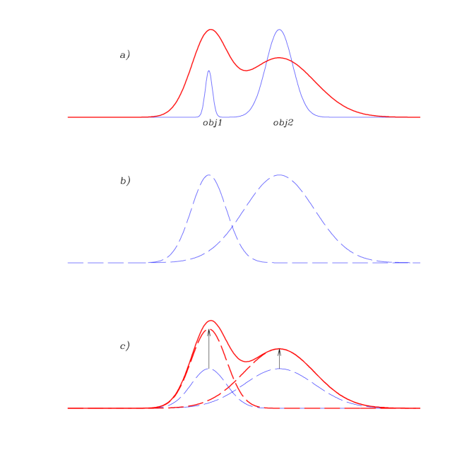
Figure 1: A schematic representation of the ConvPhot algorithm. a). Two objects are clearly detected and separated in the high resolution detection image (blue, solid-thin line). The same two objects are blended in the low resolution measure image (red, solid-thick line) and have quite different colours. b). The two objects are isolated in the high resolution detection image and are individually smoothed to the PSF of the measure image, to obtain the “model” images. c). The intensity of each object is scaled to match the global profile of the measure image. The scaling factors are found with a global $\chi^{2}$ minimisation over the object areas.

As can be appreciated from the example plotted in Fig. 1, the main advantage of the method is that it relies on the accurate spatial and morphological information contained in the “detection” image to measure colours in relatively crowded fields, even in the case that the colours of blended objects are markedly different.

Still, the method relies on a few assumptions that must be well understood and taken into account. First of all, it is assumed that the objects have no measurable proper motion. This is not a particular concern in small, deep extragalactic fields like HDF or GOODS, but might be important in other applications. A more general concern is that morphology and positions of the objects should not change significantly between the two bandwidths. Also, the depth and central bandpass of the “detection” image must ensure that most of the objects detected in the “measure” image are contained in the input catalog. Finally, the objects should be well separated on the detection image, although they may be blended in the measure image.

In practice, it is unlikely that all these conditions are satisfied in real cases. In the case of the match between ACS and ground based $Ks$ images, for instance, very red objects may be detected in the $Ks$ band with no counterpart in the optical images, and some morphological change is expected due to the increasing contribution of the bulge in the near–IR bands. This mis-match may be particularly significant for high redshift sources, where the knots of star formation in the UV rest frame are redshifted to the optical wavelengths used as model images. Also, in the case that the pixel-size of the “measure” image (i.e. ISAAC or VIMOS) is much larger than that of the “input” one (ACS for example), the actual limitations due to intrinsic inaccuracy in image aligning may lead to systematic errors.

We will show below that these effects may be minimised or corrected with reasonable accuracy: at this purpose, we have included in the code several options and fine–tuning parameters to minimise the systematics involved.

3 The ConvPhot algorithm

In this paragraph, we illustrate in detail the algorithm adopted for the ConvPhot software. Particular emphasis is given to resolve critical issues in this profile matching algorithm, such as a correct estimation of the background, an unbiased reproduction of the object profile and a fast and robust minimisation technique. We analyse in detail these critical points.

3.1 Input images and catalog

As mentioned above, ConvPhot relies on the output of the popular SExtractor code to detect and deblend the objects and to define the object position and main morphological parameters in the detection image. In the following, we shall also use the SExtractor naming convention to specify several image characteristics. We remind that a “segmentation” image is an image where background is set to 0 and all the pixels assigned to a given objects are filled with the catalog number of the object.

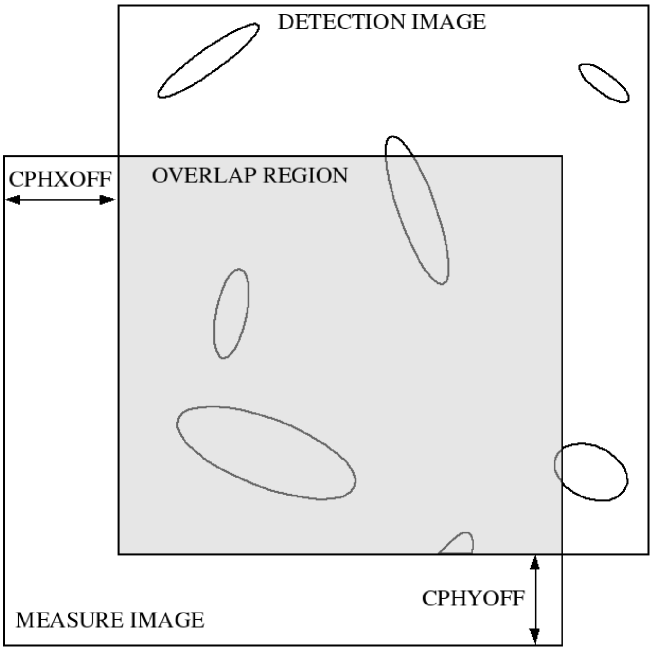
Figure 2: This figure shows how ConvPhot defines the overlap region between the detection and the measure image in case of different sizes and offsets, provided by the input parameters CPHXOFF and CPHYOFF. The objects whose segmentation is partly inside the overlap region are flagged as bound.

The user must first obtain a reliable SExtractor catalog of the detection image prior to running ConvPhot. In practice, the required output from SExtractor consists of the SEGMENTATION image and of a catalog with the center and boundary coordinates of the objects in pixel units and the value of the background, as shown in Tab. 1.

In addition to this, the user must provide the detection image and the measure with its MAP_RMS, i.e. an image containing the absolute r.m.s. of the measure image, in the same units. It is important to remind that the measure image may be shifted and/or have a different size with respect to the detection one: it is only required that the images are aligned (i.e. have been rebinned to the same pixel size and be astrometrically registered; for problems related to the rebinning of the measure image see Sect. 6). This offsetting option may be useful when dealing with the follow–up of large mosaics (i.e. GOODS, COSMOS). Fig. 2 shows the case of a measure image having a different size and shifted respect to the detection one. In this case, the relative offset (in pixels) between the two images must be provided by the input parameters CPHXOFF and CPHYOFF. The measure image and its RMS must have the same size. As shown in Fig. 2, ConvPhot works on objects whose segmentation lies in the overlapping region between the detection and the measure image. In the detection image, objects which partly lie inside the overlap region are flagged as bound and will be processed only if the fraction between the flux inside the overlap region and the total flux in the detection image is equal or larger than a user-defined parameter $f_{flux}$.

Table 1: Example of input catalog for ConvPhot.

NUMBER	X	Y	XMIN	XMAX	YMIN	YMAX	BACK_D	BACK_M
1	2319.71	216.86	2134	2507	34	384	1.350E-05	0.0
2	8849.97	79.61	8820	8881	32	124	-1.300E-06	0.0
3	5269.25	16.99	5245	5293	1	39	-6.372E-06	0.0
4	3596.99	21.14	3581	3613	5	37	-2.710E-05	0.0
5	4878.07	11.14	4852	4905	1	37	-6.634E-06	0.0

NUMBER is the identification number of the source in the segmentation image created by SExtractor, X, Y, XMIN, XMAX, YMIN, YMAX are the center and boundary coordinates of the objects (in SExtractor they are indicated as X_IMAGE, Y_IMAGE, XMIN_IMAGE, XMAX_IMAGE, YMIN_IMAGE, YMAX_IMAGE, respectively). BACK_D is the value of the background for the detection image, while BACK_M is the background for the measure image. It is possible to provide every object with its local background estimate, for example that produced by SExtractor. This example is taken from the GOODS-MUSIC catalog produced using the $z$ band provided by ACS in the GOODS South field (Grazian et al., 2006).

3.2 Small segmentation for objects

The “object segmentation” defines the area (i.e. the set of pixels) over which each object is distributed. This area, which is different in the measure and in the detection image because of the typical different image quality (PSF), is used to extract the object profile in the detection image and to define the fitting region in the measure one.

To establish the area of each object in the detection image, ConvPhot relies on the “segmentation” image produced by SExtractor. In this image, each pixel contained within the isophotal area of an object is filled with the relevant object ID, and can be used to reconstruct the shape of the object itself. This estimate, however, is not very robust since the size of the isophotal area depends on the isophotal threshold adopted in the detection image, and in any case misses a significant fraction of the flux of faint objects.

This effect is particularly dramatic as the galaxy becomes either very faint or very large, as in space based images like those provided by HST (WFPC2, ACS), with resulting low surface brightness of the external pixels. To overcome this problem, we have developed and distributed a dedicated software (named dilate), that expand the segmentation produced by SExtractor, though preventing merging between neighbouring objects and preserving the original shape of the segmentation. The segmentation of each object is individually smoothed with an adaptive kernel which preserves its shape and is then renormalised to the original number value. This software allows to fix the dilate factor $f_{DIL}$ for the magnification of the segmentation, that is defined as the ratio between the output and input isophotal area. While this procedure is useful for relatively bright objects, of which the increase of size is doubled for an $f_{DIL}=4$, it provides too small an enlargement for the faintest objects, that are often detected over very few pixels (this is particularly true in the case of faint small galaxies observed with HST, as in the case of the GOODS data). At this purpose, we allow to define a minimum area $m_{AREA}$ for the segmentation, such that objects smaller than this area (even after dilation) are forced to have this area. A minimum value for the area of extended segmentation is useful, for instance, in the ACS images, where extended but low surface brightness objects are detected by SExtractor only due to the bright nucleus and their isophotal area is limited only to the brighter knots. These values should be tuned accurately, because too small values for $f_{DIL}$ or $m_{AREA}$ may cause a distortion of the profile for the detection image, which alters the photometry in the measure image, while too large values for $f_{DIL}$ or $m_{AREA}$ are not useful since enhance the noise in the model profile. Typical values for $f_{DIL}$ are 3-4, in order to double the area of the original segmentation image. The $m_{AREA}$ parameter is set in order to match 2-3 times the typical size of galaxies in the field: for deep imaging surveys with HST, faint galaxies have an half light radius of $Rh=0.2-0.3$ arcsec, which translates to a minimum area of around 800 pixels, if the pixel scale of ACS (0.03 arcsec) is used. Moreover, ConvPhot also compute the so-called “detection magnitude”, that is the magnitude of the object in the detection image for the dilated segmentation. This quantity should be compared with the total detection magnitude of the input catalog in order to correct the model magnitude for the fraction of flux missed by the limited segmentation. In addition, the possibility of restricting the fit to the central region of the objects (as described in Sect 3.5) further suppresses the effects of tails in the fit itself.

3.3 PSF matching

A key process within ConvPhot is the smoothing of the “detection” high resolution image to the PSF of the lower resolution “measure” one. The original feature of the method is that this step is not performed on the global image, but rather on each individual object, after it has been extracted from the “detection” image, in order to prevent the confusion to to blending in low resolution images.

Such a smoothing is performed by applying a convolution kernel, that is the filter required to transform the PSF of the detection image into the PSF of the “measure” image. Filtering is performed on the thumbnails of the extracted objects, as well as on the corresponding segmentation and auxiliary images, whenever required.

The derivation of the convolution kernel is not done by ConvPhot and must be provided by the users. Several techniques have been developed to derive an accurate convolution kernel, in particular those by Alard & Lupton (1998) and Alard (2000), and we advice to use such sophisticated techniques whenever possible.

In the case of the GOODS–MUSIC sample, where we had to obtain more than 70 independent kernels (one for each original image of the J, H and K mosaics), we have adopted a simpler method, based on analysis in the the Fourier space. Such method can be implemented and automatized with standard astronomical tools for image analysis. We summarise here the basic recipe to compute it. First of all, we derive the PSF of the detection and measure image, $P_{1}$ and $P_{2}$ respectively, e.g. by summing up several stars in the field, in order to gain in Signal to Noise ratio. These two PSFs must be normalised, in order to have total flux equal to unity. The convolution kernel K is, by definition,

$$P_{2}(x,y)=K(x,y)\otimes P_{1}(x,y)\ .$$ (1)

The derivation of the exact shape of the convolution kernel is done in the Fourier space: taking ${\aleph}=FT(K)$, ${\wp}_{1}=TF(P_{1})$ and ${\wp}_{2}=TF(P_{2})$, the Fourier transform of the kernel is given by:

$${\aleph}=\frac{{\wp}_{2}}{{\wp}_{1}}\ .$$ (2)

An optimal Wiener filter (low passband filter), which suppresses the high frequency fluctuations, must be applied in the Fourier domain to remove the effects of noise. The aim of this filtering is to remove the large frequency fluctuations due to noise in the two PSFs or with scales less than the pixel scales of the input images. In order to check for the validity of the used filter, a residual is computed from the two PSFs and this must be consistent with the RMS of the coadded PSFs.

Finally, ${\aleph}$ must be anti-transformed back to the pixel space and the resulting kernel must be normalised to unity, in order to preserve the flux of the objects.

3.4 Background determination

The estimation of an accurate background is essential to determine the magnitude of faint sources. At this purpose, we have decided to adhere as much as possible to the SExtractor algorithms to compute the background of each object, and implemented several options to deal with this task. In particular, both for the detection and the measure image, the user can select one of these three options:

a) use as input a background–subtracted image, therefore relying on other applications (such as SExtractor itself) to compute the background. This option saves computing time and can be adopted when the background is quite homogeneous.

b) use the background value computed for each object by SExtractor, as stored in the input catalog (see Tab. 1).

c) Compute the background within ConvPhot: in this case, the background is computed in a “rectangular annulus” around the object, of size set by the user. Nearby objects are masked out using the dilated (see Section 3.2) segmentation map (Fig. 3).

As a background estimator, in the option c), we follow the SExtractor approach: first, the program compute the mean and median of the background pixels with an iterative $\sigma$–clipping method, until it reaches a convergence at 3 $\sigma$s, then compute the mode as $MODE=2.5\cdot MEDIAN-1.5\cdot MEAN$ and recompute the RMS of the background using the mode. If this RMS is changed by more than 20% from the previous clipped-RMS, the mean is taken as best estimate for the background, otherwise ConvPhot uses the mode. A detailed explanation of this approach can be found in Bertin & Arnouts (1996). The overall process is described in Fig.3.

The $\sigma$–clipping process is essential in rejecting pixels of possible sources not detected in the detection image but bright in the measure frame. At this purpose, the number of pixels used to compute the background should be larger than a user supplied value, the size of the “rectangular annulus”. Thus, the background estimation made by ConvPhot is time consuming since the thumbnails must be much larger than the typical size of the segmentation for the objects.

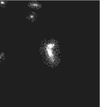
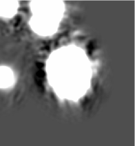
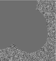
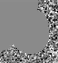
Figure 3: The procedure followed by ConvPhot to obtain the thumbnail of the local background-area of a given object. From left to right: a) the segmentation of the object and its neighbours (white) is extracted, b) the corresponding objects are extracted from the detection image, c) all the objects are smoothed to the measure PSF, defining the pixels pertaining to each source, d) the “rectangular annulus” around the object in the detection image is extracted, excluding those pixels affected by sources, and here the BACK_D value is computed e) the “rectangular annulus” around the object in the measure image is extracted as in d), and here the BACK_M value is computed.

3.5 Model profile

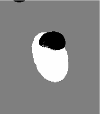
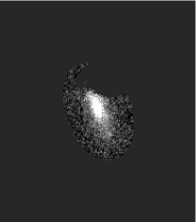
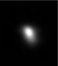
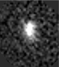
Figure 4: The procedure followed by ConvPhot to create the thumbnail of the model profile of a given object. From left to right: a) the segmentation of the object (white) is extracted, b) other objects are masked, c) the object profile is extracted from the detection image and the local background is subtracted, d) the object profile is smoothed to the measure PSF and normalised to obtain the model profile, e) the same object is extracted from the measure image subtracting its local background.

ConvPhot creates a model profile of each object, whose segmentation lies inside the overlap region, to measure the colour of the object itself. In the procedure, depicted in Fig. 4, the (dilated) segmentation of the object is extracted from the segmentation image and stored in a thumbnail. The value of the pixels relative to the given object are set to 1 while the pixels of other objects and of the background are masked setting them to 0. Using this masked segmentation, that defines the isophotal area, the object is extracted from the detection image and its background, provided by the input catalog or estimated by ConvPhot itself as described above, is subtracted producing the object profile which is stored in a new thumbnail and smoothed to the seeing of the measure image with the PSF–matching kernel. If the object is flagged as bound the total flux $D_{i}^{bound}$ is computed and the thumbnail is resized extracting only the pixels inside the overlap region (Fig. 2). Then, the thumbnail isoarea and total flux $D_{i}$ are computed from the detection image. For a bound object, ConvPhot estimates the fraction of total flux $D_{i}/D_{i}^{bound}$ inside the overlap region and if this value is less than $f_{flux}$ (by default 0.4), it rejects the object. Finally, the thumbnail is normalised to unit flux obtaining the model profile of the object. The total flux $D_{i}$ will be used later to obtain self–consistent colours.

For the reasons described below, it may be useful to perform the fitting procedure only on the central part of the profile: at this purpose, we have introduced the threshold parameter $t_{f}$, such that only the pixels above the relative threshold $t_{i}=P_{i}^{max}*t_{f}$ are used, where $P_{i}^{max}$ is the model profile maximum. Finally, ConvPhot uses the isophotal area of the (selected) model profile to extract the same object from the measure image subtracting its local background and producing a measure thumbnail with the corresponding RMS thumbnail.

3.6 Minimisation procedure

We now describe the minimisation process, making explicit use of the same notation adopted in FSLY99.

Given the model profiles (the selected model profiles if the threshold $t_{f}$ has been used) of each object $P_{i}(m,n)$, the minimisation procedure aims at obtaining the scaling factors $F_{i}$ (i.e. the fitted flux of the object in the measure image assuming as object profile the model image) of each object that best reproduce the measure image $I$. The best fit solution will be found by minimising the $\chi^{2}$, that reads:

$$\chi^{2}=\sum_{m,n}\left[\frac{I(m,n)-B_{i}-M(m,n)}{\sigma(m,n)}\right]^{2}$$ (3)

where

$$M(m,n)=\sum_{i=1}^{N_{\rm obj}}F_{i}P_{i}(m,n)$$ (4)

is the sum of all profiles, $B_{i}$ is the background (in the measure image) fitted for each objects, $\sigma(m,n)$ is the r.m.s. of the measure image and $m$ and $n$ run over all the pixels.

The best–fit solution is found by solving the linear system:

$$\frac{\partial\chi^{2}}{\partial F_{i}}=0\;\;\;(i=1,\ldots,N_{\rm obj})$$ (5)

whose Hessian matrix is

$$A_{ij}=\sum_{m,n}{\frac{P_{i}(m,n)P_{j}(m,n)}{\sigma(m,n)^{2}}}$$ (6)

and right–hand term is:

$$R_{i}=\sum_{m,n}\frac{P_{i}(m,n)[I(m,n)-B_{i}]}{\sigma(m,n)^{2}}.$$ (7)

Since the products of the model profiles are non–zero only within the area provided by the (dilated) segmentation map, most of the $A_{ij}$ terms are actually null (non–null terms will correspond to overlapping objects), such that the matrix $A$ is very sparse. The solution of linear systems is performed by an LU decomposition using the GNU Scientific Library (GSL) and its LAPACK routines (Anderson et al. 1999), such that the solution can be obtained even for a large number of free parameters (that is, of detected objects) that typically occur in deep HST exposures (i.e. UDF, GOODS or COSMOS surveys).

Finally, the statistical uncertainties on the fitted parameters $F_{i}$ are the diagonal terms of the inverse of the Hessian matrix $A_{ij}$, which depend on the RMS of the measure image and on the model profile. In a sense, this fitting procedure is equivalent to derive a profile-weighted flux and error, relying on the model image.

3.7 Output quantities

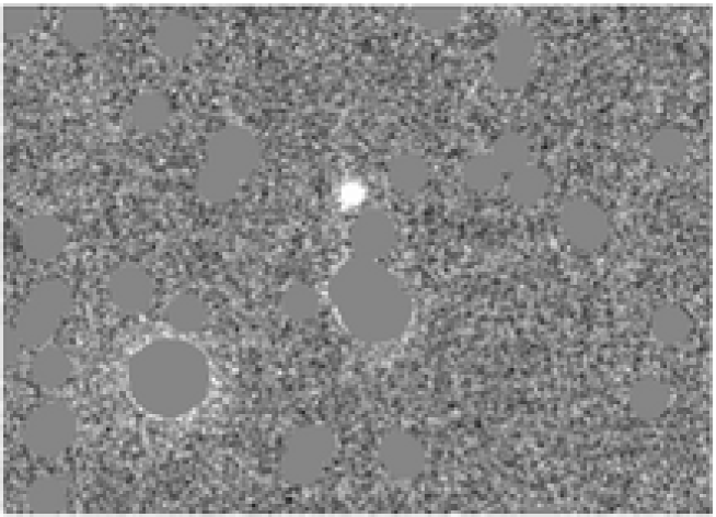
Figure 5: A so-called “Drop” image produced by ConvPhot after the fitting procedure. The name illustrates that each object detected in the high resolution image, and hence fitted by ConvPhot, is multiplied by zero: this allows to identify objects in the measure image (“drop”–out objects) that were not detected in the detection one.

ConvPhot produces in output several quantities, including parameters for each object as well as several type of images.

The most important output quantities are the best–fit solutions of the minimisation procedure, i.e. the $F_{i}$ parameters and their relative errors. Since the $P_{i}$ model for each object is normalised to unit flux, the resulting total magnitude in the measure image is simply $-2.5\log(F_{i})+ZP_{m}$, where $ZP_{m}$ is the zero-point of the measure image itself. Based on our tests, we have concluded that this total magnitude is a reliable measure of the actual total flux of the objects, somewhat less prone to systematic effects than the Kron magnitudes computed by SExtractor. However, these total magnitudes can be hardly compared with the SExtractor magnitudes of the detection image, so that reliable colours cannot be directly obtained. A robust colour estimation, indeed, should be carried out on a same area of the object and possibly be extended to a large region of the source, in order not to be biased by red nuclei (typical of bulges or elliptical galaxies) or by strong colour gradients, especially in the rest frame UV wavelengths. At this purpose, we use the total flux $D_{i}$ measured by ConvPhot itself in the detection image as a good estimate for the flux of the detected object, and used it to normalise the object profile $P_{i}$. The resulting flux ratio is therefore $Flux(measure)/Flux(Detection)=F_{i}/D_{i}\times 10^{-0.4(ZP_{m}-ZP_{d})}$, where $ZP_{d}$ and $ZP_{m}$ are the zero-points of the detection and measure image, respectively. This flux ratio, or the equivalent colour, $m_{measure}-m_{detection}=-2.5\log(F_{i}/D_{i})+ZP_{m}-ZP_{d}$ is the fundamental output of ConvPhot. These useful quantities are saved in the ConvPhot output files, as well as the background estimations, the area used during the fitting procedure, the goodness of the fit and the residuals left in the measure image.

In addition, ConvPhot produces useful output images, such as the model image $M(m,n)$ with each object scaled to the fitted flux. In particular, we produce a “Residual” image, containing the fit residuals, i.e. the quantity ${I(m,n)-B_{i}-M(m,n)}$. This image is useful to judge the quality of the fit and the background estimation. Since large residuals could typically occur in the center of bright objects, this image is not very useful to perform an automated search of objects that are detected only in the measure image but are not present in the detection image (called “dropout”). At this purpose, ConvPhot also produces a “Drop” image, where all the pixels within the (dilated) segmentation are set equal to zero. The example in Fig. 5 is taken from the K band image of the GOODS South field (Grazian et al., 2006), where a galaxy remains in the “Drop” image after the fitting of objects selected in the $z$ band of ACS.

4 Blended sources in the detection image

The ConvPhot algorithm is ideally suited for photometry of blended objects on the measure image, but requires that the same objects in the detection image should be well defined and their profiles are not distorted by noise. In the practical case, even in the GOODS-ACS images, there are galaxies blended in the ACS images or faint objects, brighter than the detection limit but still affected by noise in their shape/profile. To overcome the risk of bad modelling for these sources, we introduce in ConvPhot an option to carry out the fitting procedure only on the central part of the profile: the fit is restricted only to the pixels where the detection image is above a given relative threshold $t_{f}$. This ensures that the fit is carried out only where the Signal to Noise of the model (detection image) is high and avoids the contamination from nearby sources, which cannot be perfectly modelled in the detection image.

The effects of source blending on the detection image is investigated by means of simulations. Fig.6 and Fig.7 reproduce two elliptical galaxies (with half light radius of 0.3 arcsec and ellipticity 0.5) with different angular separations (between 0.5 and 2.0 arcsec) and show the difference between the input colour and the output of ConvPhot, $\Delta C=(z-Ks)_{out}-(z-Ks)_{inp}$. The characteristics of the detection image reproduces the $z$ band of ACS for the GOODS South field (FWHM=0.12 arcsec, pixel scale=0.03 arcsec), while the measure image fits the ISAAC $Ks$ band (FWHM=0.5 arcsec and pixel scale of 0.03 arcsec to match the ACS frame). The RMS is chosen equal to the typical value of GOODS $z$ band images (the $rms$ is 0.0014 ADU$/$Pixel), both for the detection and the measure images and is added to the synthetic frames with the IRAF task mknoise. The two galaxies are relatively bright in the $z$ band (magnitude 21 and 24 in the AB photometric system), and have $z-Ks$ colours typical of local ellipticals ($z-Ks=1$ and 2). We simulate 10 pairs of galaxies for each angular separation in order to have enough statistics in the output quantities. The colour of the brighter source is recovered within few millimag even if the two sources started to be blended in the detection image. The magnitude of the fainter galaxy, however, is affected by light coming from the bright neighbour, which produce a difference $\Delta C=-0.1$ in colour at small angular separations ($\leq 1^{{}^{\prime\prime}}$).

Fig.8 and Fig.9, indeed, describe the effects of blending in an extreme case, where the fainter galaxy in the detection image has a $z-Ks$ colour equal to 5, typical of an Extremely Red Object (ERO), which reproduces the typical colours of ellipticals at intermediate redshifts (Daddi et al., 2000). In this critical situation, the difference between the simulated and ConvPhot colour is 0.15-0.2 at a separation of 0.5 arcsec, and the fitting procedure left visible residuals. It is important to remark that the fit remains accurate as long as the two objects are separated in the detection image (i.e. for distances larger than 1.0 arcsec), although they are already blended in the measure image. As the sources become deeply blended in thedetection image, with distance less than 1.0 arcsec, a non-negligible contamination starts to appear. Not surprisingly, such contamination is larger for the bluer and fainter (in Ks) galaxy. Fortunately, this situation is not common even in large and deep areas like the GOODS survey, and even for faint objects in the detection image the magnitude in the measure image is recovered with acceptable accuracy. We have to stress that in this case the parameters of the dilate and ConvPhot softwares (dilation factor, minimum area, threshold, background annulus) are not optimised for this special case but are the standard values used for all the simulations in this paper.

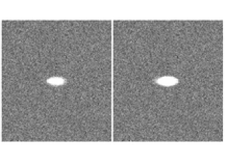
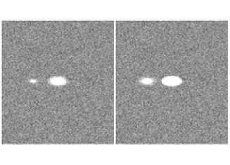
Figure 6: The effect of blending on the detection image in a standard case. Two elliptical galaxies with $Rh=0.3$ arcsec are simulated as a function of the angular separations in order to study the combined effect of blending and colours. One object is a relatively bright, blue galaxy ($z=21$, $z-Ks=1$), the second is a fainter, slightly redder galaxy ($z=24$, $z-Ks=2$). The detection image has the pixelscale and noise properties of the ACS GOODS images (seeing=0.12, pixel scale=0.03 arcsec), while the measure image reproduces the typical properties of a Ks band image of the GOODS data set, with a FWHM seeing of 0.5 arcsec. For each separation we computed 10 different realization of the galaxy pairs. In the upper panel, bi-dimensional images of the galaxies with a separation of 0.5 arcseconds (two leftmost images) and 2.0 arcseconds (two rightmost images) are shown. In both cases, the first (left) thumbnail is the $z$ band, while the second is the Ks band. In the lower panels we plot the difference between the input and derived colours ($\Delta C$) for faint and bright sources as a function of the angular separation. Even when the sources are deeply blended, the error on the estimated colour for the fainter galaxy remains acceptable ($\simeq 0.1$ mags).

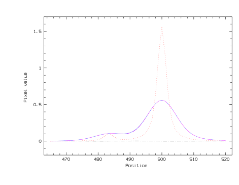
Figure 7: A blending case is simulated (upper left panel of Fig.6), with distance of 0.5 arcsec between the two peaks, for the objects described in Fig. 6. The position is given in pixel units and the pixel scale is 0.03 arcsec. Solid lines shows the $Ks$ profile, dotted line the $z$ band profile, long-dashed line the fit provided by ConvPhot and the dot-dashed line represents the residual. The fitting procedure succeeds in recovering the true flux, as the flat residual demonstrates.

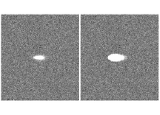
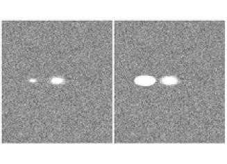
Figure 8: Simulations on the effect of blending on the detection image in a case of extreme colours. Similar to Fig.6, two elliptical galaxies with $Rh=0.3$ arcsec are simulated as a function of the angular separations in order to study the combined effect of blending and colours. At variance with Fig.6, colours are so extreme here that the object that is fainter in the detection image is indeed brighter in the measure one. Specifically, one is a relatively faint, blue galaxy ($z=22$, $z-Ks=1$), the second is a fainter but much redder galaxy ($z=24$, $z-Ks=5$), in order to simulate an Extremely Red Object. The detection image has the pixelscale and noise properties of the ACS GOODS images (seeing=0.12, pixel scale=0.03 arcsec), while the measure image reproduces the typical properties of a Ks band image of the GOODS data set, with a FWHM seeing of 0.5 arcsec. For each separation we computed 10 different realization of the galaxy pairs. In the upper panel, bi-dimensional images of the galaxies with a separation of 0.5 arcseconds (two leftmost images) and 2.0 arcseconds (two rightmost images) are shown. In both cases, the first (left) thumbnail is the $z$ band, while the second is the Ks band. In the lower panels we plot the difference between the input and derived colours ($\Delta C$) for faint and bright sources as a function of the angular separation. It is shown that the fit remains accurate as long as the two objects are separated in the detection image (i.e. for distances larger than 1.0 arcsec), although they are already blended in the measure image. As the sources become deeply blended in thedetection image, with distance less than 1.0 arcsec, a non-negligible contamination starts to appear. Not surprisingly, such contamination is larger for the bluer and fainter (in Ks) galaxy.

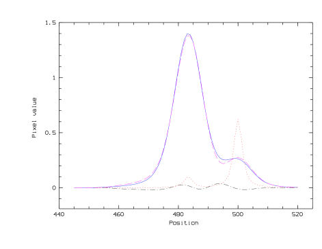
Figure 9: A deep blending case is simulated, with distance of 0.5 arcsec between the two peaks, for the objects described in Fig. 8. One object has an extreme colour ($z-Ks=5$). The position is given in pixel units and the pixel scale is 0.03 arcsec. Solid lines shows the $Ks$ profile, dotted line the $z$ band profile, the long-dashed line the fit provided by ConvPhot and the dot-dashed line the residual.

5 Systematics in the PSF-matching

We briefly describe here the systematics that may affect such PSF–matching procedure and the approaches that we have developed within ConvPhot to minimise them.

Alignment errors
The fitting procedure is extremely sensitive to alignment errors. In the simple case that the object has a 2–D Gaussian shape of standard deviation $\sigma$ ($=FWHM/2.3548$), it is easy to show that the resulting flux is systematically underestimated by a factor $f=exp(-\frac{3}{4}\frac{\Delta r^{2}}{\sigma^{2}})$, where $\Delta r$ is the offset in pixel of the center position. When ground–based images are combined to HST images with excellent sampling, this effect is non-negligible. In the case of the GOODS ACS data, for instance, the ACS pixel-size is 0.03”, that is often smaller than the residuals of the alignment of IR ground–based images. For an alignment error of 1 pixel (in the detection image), a figure that can be quite typical or even optimal when combining ground–based and HST images, the resulting flux underestimate may be of about 3%.

As a first way out, we have included in ConvPhot an option to re-center any object before minimisation. In this case, the center of each object are internally computed in the model as well as in the measure image, and the measure is re-centered to the model image before minimisation. Since the center determination may be noisy for faint objects, the user can set a limit on the S/N of the objects (in each image) to execute this operation only on bright sources. We remark that such option must be adopted with great care, after tests and simulations on the specific data. In the case of the GOODS–MUSIC catalog, for instance, we have adopted the recentering option for sources with $S/N\geq 15$ both in the model and in the measure image for the WFI U bands, while we decide not to use this option for U-VIMOS, ISAAC and IRAC data.

Variable FWHM or object profile
Another source of uncertainty may result from a variation of the object profile from the detection to the measure image. This can be due to either a physical change of the object profile (as due, for instance, to a more prominent bulge in the IR) or to an incorrect estimate of the PSF transformation kernel. In this case, assuming that the profile of an isolated objects in the model image and in the measure image are both Gaussian with same center and different $\sigma$, the resulting flux is incorrectly estimated by a factor $f=2\sigma_{model}^{2}/(\sigma_{model}^{2}+\sigma_{measure}^{2})$. In this case, the resulting flux can be therefore either under- or over-estimated, depending on the sign of the error in the PSF estimate. An error of 10% in the object PSF will result in a 5% error in the output flux.

The small systematic effects that have been described above, or others resulting from different sources, can be efficiently corrected by taking into account the flux in the residual image. At this purpose, we have included in the code an option to compute the total residual flux contained in the segmentation area of the original frame. This correction is computed in a small region in order not to be affected by nearby objects, which would drastically contaminate the corrections computed in the residual image, especially for faint objects severely blended with bright sources in the measure image. In Fig. 10 we show the efficiency of using the residuals to correct possible biases due to centering problems.

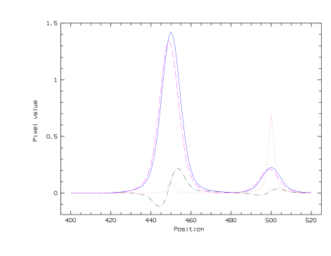
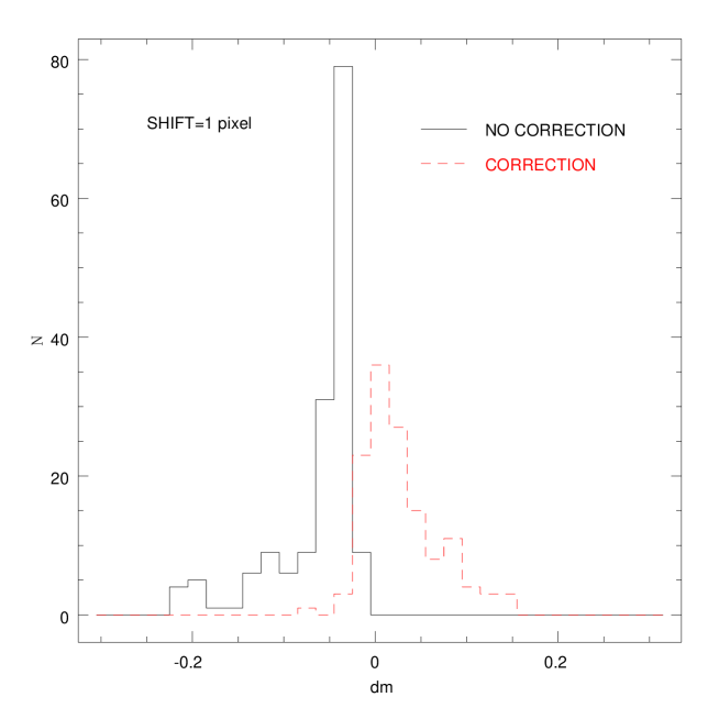
Figure 10: The effect of not accurate centering of the detection and measure images. The two objects are the same as in Fig. 8 but with a distance of 2 arcsec (upper panel). The $z$ and $Ks$ images are shifted of 1 pixel. The position is given in pixel units and the pixel scale is 0.03 arcsec. The lower panel shows the difference between input and measured colours without correction (solid histogram) and taking into account the correction provided by ConvPhot (dashed line).

Objects with low Signal to Noise Ratio
A well known drawback of our procedure occurs when the objects have a low S/N in the detection image, since this would result in a noisy determination of the profile, and hence of the final colour, even for objects that have a high S/N in the measure image. During the development of ConvPhot, we indeed considered the possibility of using some parametric fit as input shape of the objects. After some test (which revealed also that the task is computationally heavy), we realized that it was not a viable solution, for two reasons:

• 1) a large fraction of faint galaxies have intrinsically irregular morphologies, such that errors in their fitting produces at least the same level of uncertainty or worse than using their observed profile, albeit noisy;

• 2) for faint objects, the PSF-match smoothing significantly reduces the noise, such that the leading error term is anyway the global uncertainty on the total flux, that is also present at the same level in the parametric fitting of the shape.

For these reasons, we did not insert such technique in ConvPhot.

6 Validation tests

We have performed several validation tests on the ConvPhot code, during the debugging phase and to estimate the efficiency in the correction for systematics.

6.1 Test on simulated data

A first, obvious set of simulations has involved the use of synthetic images, obtained with the IRAF ARTDATA package, where we have simulated either single or pairs of galaxies of various luminosities, morphologies and resolutions, by which we have verified that the code is computationally correct. Examples of this simulations are those reproduced in Fig.6 and Fig.8 and will not be presented here.

We have done more accurate tests to validate ConvPhot when dealing with the complexity of real data. First of all, we checked the reliability of ConvPhot simulating the typical case of an HST deep image as detection and a ground based image as measure, using three cutouts of the real ACS images of the GOODS-South field. As detection image, we have used the original $z$ band (F850LP, 0.12 arcsec FWHM), with its relative segmentation map and SExtractor photometry derived by the GOODS-MUSIC database (Grazian et al., 2006). As measure images, we have smoothed the $B$ (F435W) and $I$ band (F775W), with a 0.5 arcseconds kernel. We have run ConvPhot only on sources that are fully inside the measure images ($f_{flux}=1$), expanding the thumbnails of 128 pixels in order to have enough pixels to compute the background with ConvPhot, and with threshold 0.0 and 0.5 (with the latter choice we fit only the central part of the objects).

As a figure of merit, we compare in Fig. 11 the $I-Z$ and $B-Z$ colours obtained by ConvPhot with the aperture colour obtained by SExtractor on the original, high resolution images, that are those used in (Grazian et al., 2006).

At first glance, this plot shows that our software is not biased in the colour determination for bright as well as for faint sources. Looking into the details, the residuals of the colours show a different behaviour for bright ($Z_{sex}\leq 23$) and faint galaxies. The residuals of the bright sub-sample have larger dispersion both in the B band and in the 0.5 threshold cases: an investigation by eye of these bright sources with large scatter in the colour residuals indicates that the main reason is the morphological change of source profile for nearby bright galaxies, as for example that in Fig. 12. The profiles of nearby and bright galaxies differ largely when observed in the near UV and in the near IR, since in the UV the star forming regions are clearly visible, and their spatial distribution is significantly different than the regions occupied by old/evolved stars, which emit mainly in the near IR. In this case, if the galaxy profile in the $Z$ band is used to derive the magnitude of the source, it will result in a slightly poorer fit, especially when the wavelength different is large (B vs Z bands) or when the fit is restricted to the small central bulge (threshold=0.5).

For faint sources, however, the difference between the $B-Z$ and $I-Z$ is not significant, while an higher threshold is useful to enhance the quality of the fit and the accuracy of the magnitude estimation.

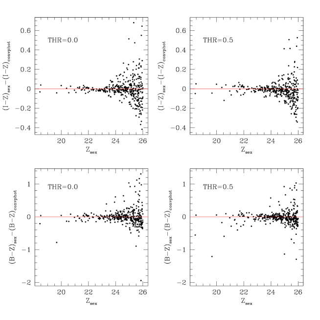
Figure 11: The $I-Z$ and $B-Z$ colours as a function of the $z$ band magnitude of the objects detected on the GOODS-South survey. Two different values of the threshold are used (0.0 and 0.5) and they affect in dissimilar way the bright and faint objects. The small scatter in the input and ConvPhot colours shows that the ConvPhot colour determination is not biased and is compatible with aperture photometry.

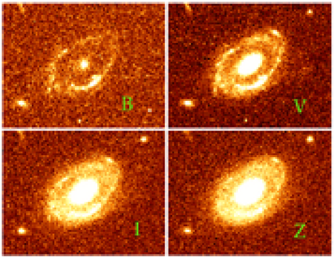
Figure 12: A nearby galaxy in different optical bands (B,V,I,Z) taken from the GOODS-MUSIC database. The different morphologies indicate the predominance of star-forming regions in the B band in a ring around the galaxy disk and the compactness of the old stellar population in the Z band in the bulge.

6.2 Real data

Simulations, however, cannot reproduce the complexity of real objects and data. To obtain a more stringent and independent test we have made use of the $z$ band FORS image of the K20-CDFS (seeing=0.55 arcsec and pixel scale=0.2 arcsec). We have already analysed the K20 data set in a previous paper (Cimatti et al 2001), applying a standard technique based on aperture photometry obtained with SExtractor. Here, we have used ConvPhot to obtain a new estimate of the $z_{ACS}-z_{FORS}$ colour in the FORS image of the K20, and compared them with the previously published catalog. To this aim, we have used the GOODS ACS z-band image as detection, with a typical FWHM of 0.12 arcsec and pixel scale of 0.03 arcsec. The results of this test are shown in Fig.13, which are not corrected for the small offset in the average colour ($<z_{ACS}-z_{FORS}>=0.05$) due to the small difference in the filter response curve. Once allowing for this offset, the plot shows that ConvPhot is not biased in the colour estimate in respect to standard aperture photometry.

Figure 13: The $z_{ACS}-z_{FORS}$ colour as a function of the magnitude of the objects detected on the K20 survey (upper panel). The histogram of this colour (lower panel) shows that the ConvPhot colour determination is not biased and is compatible with aperture photometry.

6.3 An extreme example: the case of MIPS data

We have also made extensive tests in a case when ConvPhot is pushed to its very limits, i.e. when the resolutions, pixel scales and wavelengths of the two images are very different. Such a situation is very challenging both conceptually and technically, since the present version of ConvPhot works on detection and measure images after aligning and rebinning them to the same pixelscale and reference frame (a discussion on future possible improvements is given in the following). At this purpose, we have taken the extreme case of applying ConvPhot to a combination of HST–ACS and Spitzer–MIPS images which have pixel scales of 0.03 and 1.2 arcsec/pixel, respectively. Such data set is again taken from the public data of the GOODS survey, where we take again the ACS $z$ band as detection image and the MIPS image at $24\mu m$ as measure.

In principle, we should align and resample the original MIPS images, with a typical PSF of 5.2 arcsec, at the same scale of the ACS ones. This would result in a minimum size of the resulting thumbnail of $2000\times 2000$ pixels, that would make impracticable the use of ConvPhot even with fast workstations. To circumvent this problem, we rebinned the ACS detection image by a factor $8\times 8$ (0.24 arcsec/pixel), resulting in a severely undersampled image (the FWHM of the ACS GOODS image is 0.12 arcsec), reducing significantly the image size. We also rebinned of the same amount (with a specific code) the input Segmentation image. Finally, we aligned and rebinned the MIPS data to such a rebinned ACS image. The advantage of this procedure is that the requirements of memory and CPU time are significantly reduced, although we loose some information when introducing a undersampling of the original image.

Before applying it to the real data, we performed a simulation by smoothing the rebinned ACS image to the same PSF of the MIPS data, and used ConvPhot to estimate the colour between the original and the MIPS–smoothed one. Fig. 14 shows the comparison between the input and the ConvPhot magnitudes, indicating that this software can be used even when dealing with such extreme cases. This plot shows also that the thresholding option for ConvPhot can be useful to reduce the scatter of the magnitude estimation.

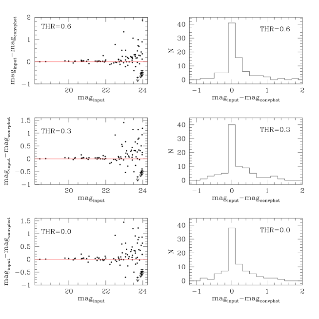
Figure 14: Results of the simulations which reproduce the $z$ band of ACS and the 24 micron band of MIPS as detection and measure images, respectively. The y–axis shows the difference between the input magnitudes and those derived by ConvPhot as a function of the magnitude on the simulated objects. The simulated image is derived by smoothing the original $z$ band, so that the expected colour should be zero. The histogram of the colours (right panels) shows the result for different value of the threshold in ConvPhot. Arrows indicate upper limit in the ConvPhot magnitude.

We finally obtained a MIPS catalog of all sources in the GOODS–MUSIC sample, after rebinning the original ACS z-band detection and segmentation images by a factor of 8, computing the appropriate kernel and run ConvPhot over the entire GOODS field. We have used a threshold of 0.3 and an $f_{flux}$ factor of 0.2, on the indications of the simulations described in the previous section.

To check the reliability of our magnitude estimation in the real MIPS image, we compare the ConvPhot magnitude estimate with those derived by SExtractor. These are computed on circular apertures of 6 and 6.6 arcsec radius, and then corrected applying an appropriate correction factor given in the MIPS Instrument Manual, in this case 0.58 and 0.54 magnitudes, respectively. The corrected aperture magnitudes are an unbiased estimate of the true source luminosity only if the object is isolated. Obviously, given the large FWHM of the MIPS 24 micron Point Response Function (or PSF), the effect of crowding on the aperture magnitude is severe for faint sources, typically at $mag\geq 19$.

Fig. 15 shows the comparison between the corrected aperture magnitudes and those derived by ConvPhot for the entire GOODS-South field, indicating that even in the real case our algorithm retrieve the correct fluxes. If a comparison is made with the photometric catalog released by the GOODS Team (Chary et al., in prep.), who used a similar technique starting from the IRAC 3.6 micron as detection image, we find a good agreement for relatively bright objects. This indicates that our background estimation is correct and the ConvPhot result is robust. After the comparisons both with simulations and real data, we are thus confident that the ConvPhot algorithm is stable even in this extreme case, both due to the wavelength and PSF differences between the detection and measure images.

A final remark is necessary about the use of undersampled image. We have made a test using undersampled images (obtained by rebinning the usual GOODS–$z$ band image by a factor 8), and simulated a ground based image with seeing of 0.5 arcsec. In this case, we found evidence that the ConvPhot magnitudes are significantly biased, with a typical underestimate of the fitted flux by 0.2 magnitudes. We therefore conclude that - not surprisingly - the use of undersampled images as detection images should be avoided when the difference in resolution and pixelscale is less extreme than the MIPS case described above..

This is just an example of how much the use of this software however is delicate. We therefore strongly recommend the interested user to make a set of realistic simulations to check the effect of the multiple parameters on the correct magnitude estimation.

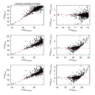
Figure 15: The difference between the SExtractor aperture magnitude, corrected for the flux fraction missed by the small circular aperture, and the magnitude derived by ConvPhot for the MIPS 24 micron sources in the GOODS-South field. The histogram of the magnitude residuals shows that the ConvPhot colour determination is not biased, while the comparison of the ConvPhot magnitudes with those derived by Chary et al. (in prep.) shows a small (0.1 mag) offset.

7 Known ConvPhot issues: room for improvement

The present version of ConvPhot has several limitations, which are described here and will be solved in future versions of this software. We summarise the most important in this brief list, and defer to future version of the Code their implementation.

• A major limitation results from the fact that all the thumbnails of the processed sources are stored in the computer memory. This allows to carry out the computation faster but limits the size of the images on which ConvPhot operates.

• The measure image and its RMS must be rebinned to the detection image reference frame. In this case the alignment between sources can be done accurately using dedicated routines (i.e. swarp, IRAF) and the advantage of dealing with small pixel scales is to carry out a fine tuning of the source centering in ConvPhot. A draw back is that it increases the thumbnail dimensions and consequently reduce the number of sources to be stored in the computer memory. A possible way out would be to avoid at all any rebin, and work directly in astrometric coordinates.

• If two sources are blended in the detection image their profiles in the model image will be different from the real case. A modelling of the object profile for blended sources is definitely needed, but its implementation is not easy, especially for irregular sources.

• The convolution with the input kernel is performed in pixel space, which is computationally an heavy process. A convolution in the Fourier space would allow a much faster computation.

• The kernel derivation is left to the user and it is fixed for all the sources in an image. It is not foreseen for the moment the possibility of compute the smoothing kernel internally or using a PSF which varies according to the position of the objects.

• The recentering option is very simple, since it takes the maximum of a source in the detection and measure image and compute the relative shifts. This is not accurate for the case of crowded fields or large PSF images, in which a mis-identification of two close sources turns out in a wrong magnitude estimation.

• The option to correct the fitted flux with a statistic of the residual image in the original segmentation is not satisfactory when dealing with large kernel, and more simulations are necessary to find a proper solution for these cases.

8 Summary and Conclusion

We have described in this paper a new, public software for accurate multiband photometry of images of different resolution and depth, that we have named ConvPhot. The code is based on an algorithm that has been originally proposed by FSLY99 and applied in some previous analysis of deep extragalactic imaging data (Lanzetta et al., 1999; Papovich et al., 2001). The code performs a “PSF-matched” photometry on two images with different PSF, by first extracting all objects from the first (detection) image, smoothing each of them to the PSF of the second (measure) image, and obtaining the flux of each object on the measure image by a global $\chi^{2}$ minimisation over the whole image.

We provide here for the first time a public version of such a code, of which we discuss the basic algorithm, the possible systematic effects involved and the results of a set of simulations and validation tests that we have performed on real as well as simulated images. To maximise the usability of the code, we explicitly use the outputs of the popular SExtractor code as inputs to our procedure.

This code has been extensively used and tested to obtain the GOODS–MUSIC sample, based on the public release of the GOODS–South data, as we have described in Grazian et al. (2006). In such a context, we used ConvPhot to obtain colours for more than 18000 sources originally detected in a wide, high resolution mosaic of HST-ACS images. It has proven to be reliable enough to flawlessly process around 70 frames at different wavelengths and image quality and depth, ranging from VLT–VIMOS images in the U band (with typical PSF of 1”) to VLT–ISAAC images in J, H and K (with typical PSF of 0.5”), as well as Spitzer-IRAC images (with typical PSF of 2”). We believe that the number of options in the code make it flexible enough for a wider use.

ConvPhot is written in C language under the GNU Public License and is publicly released worldwide. This software is described in detail in a WEB site where the source code can be retrieved, together with the user manual: http://lbc.oa-roma.inaf.it/convphot.

Acknowledgements

We warmly thank the referee, M. Strauss, for his useful suggestions and comments, that largely improved the quality and amount of information in this paper. It is a pleasure for us to warmly thank Giulia Rodighiero for her patience during the software testing/usage and for very useful comments to improve this paper, the ConvPhot software and its user manual.

References

- Alard (2000) Alard, 2000, A&AS 144, 363
- Alard & Lupton (1998) Alard, Lupton, 1998, ApJ 523, 325
- Anderson et al. (1999) Anderson, E., Bai, Z., Bischof, C., Blackford, L. S., Demmel, J., Dongarra, J., Du Croz, J., Greenbaum, A., Hammarling, S., McKenney, A., Sorensen, D., 1999, LAPACK Users’ Guide (Third Edition), Society for Industrial and Applied Mathematics
- Bertin & Arnouts (1996) Bertin, E. & Arnouts, S. 1996, A& AS, 117, 393
- Chary et al. (in prep.) Chary et al. in preparation.
- Cimatti (2001) Cimatti, A. 2001 Deep Fields, Proceedings of the ESO/ECF/STScI Workshop held at Garching, Germany, 9-12 October 2000. Stefano Cristiani, Alvio Renzini, Robert E. Williams (eds.). Springer, 2001, p. 81.
- Daddi et al. (2000) Daddi, E., Cimatti, A. & Renzini, A. 2000 A& A, 362L, 45
- Dickinson et al. (2003) Dickinson, M., Papovich, C., Ferguson, H.C., Budavari, T., 2003, ApJ 587, 25
- Fernandez–Soto et al. (1999) Fernández–Soto, A., Lanzetta, K. M., Yahil, A. 1999, ApJ, 513, 34; FSLY99
- Fontana & Ballester (1995) Fontana A. & Ballester P., 1995, ESO The Messenger 80, 37.
- Fontana et al. (2000) Fontana, A., D’Odorico, S., Poli, F., Giallongo, E., Arnouts, A., Cristiani, S., Moorwood, A., & Saracco, P. 2000, AJ, 120, 2206
- Grazian et al. (2006) Grazian, A., Fontana, A., De Santis, C., et al., 2006, A& A, 449, 951
- Lanzetta et al. (1999) Lanzetta, K. M., Chen, H. W., Fernández–Soto, A., Pascarelle, S., Yahata, N., Yahil, A. 1999 ASPC, 193, 544
- Papovich et al. (2001) Papovich, C., Dickinson, M. & Ferguson, H. C., 2001, ApJ, 559, 620
- Phillipps et al. (2000) Phillipps, S., Driver, S. P., Couch, W. J., Fernández–Soto, A., Bristow, P. D., Odewahn, S. C., Windhorst, R. A., Lanzetta, K. 2000, MNRAS, 319, 807
- Poli et al. (2001) Poli, F., Menci, N., Giallongo, E., Fontana, A., et al., 2001, ApJL 551, 45
- Schechter et al. (1993) Schechter, P. L.; Mateo, M.; Saha, A. 1993 PASP, 105, 1342
- Szalay, Connolly & Szokoly (1999) Szalay, A. S., Connolly, A. J., Szokoly G. P. 1999, AJ, 117, 68