An idealized model for dust-gas interaction in a rotating channel

Abstract

A 2D model representing the dynamical interaction of dust and gas in a planetary channel is explored. The two components are treated as interpenetrating fluids in which the gas is treated as a Boussinesq fluid while the dust is treated as pressureless. The only coupling between both fluid states is kinematic drag. The channel gas experiences a temperature gradient in the spanwise direction and it is adverse the constant force of gravity. The latter effects only the gas and not the dust component which is considered to free float in the fluid. The channel is also considered on an f-plane so that the background vorticity gradient can cause any emerging vortex structure to drift like a Rossby wave. A linear theory analysis is explored and a nonlinear amplitude theory is developed for disturbances of this arrangement. It is found that the presence of the dust can help generate and shape emerging convection patterns and dynamics in the gas so long as the state of the gas exceeds a suitably defined Rayleigh number appropriate for describing drag effects. In the linear stage the dust particles collect quickly onto sites in the gas where the vorticity is minimal, i.e. where the disturbance vorticity is anticylonic which is consistent with previous studies. The nonlinear theory shows that, in turn, the local enhancement of dust concentration in the gas effects the vigor of the emerging convective roll by modifying the effective local Rayleigh number of the fluid. It is also found that without the f-plane approximation built into the model the dynamics there is an algebraic runaway caused by unrestrained growth in the dust concentration. The background vorticity gradient forces the convective roll to drift like a Rossby wave and this causes the dust concentration enhancements to not runaway.

1 Introduction and summary of results

There has been growing interest in recent years in the possibility that persistent vortex structures in protoplanetary discs may be the sites where planetesimals are formed (Barge & Sommeria, 1995, Tanga et al., 1996, Bracco et al, 1999, Barranco & Marcus, 2000, Barranco & Marcus, 2006). These investigators have put forth the scenario in which a disc, laden with dust, supports some type of long-lasting vortex (driven by some unspecified excitation mechanism, except for Klahr & Bodenheimer, 2003 and Barranco & Marcus 2006) that manages to attract the dust through the combined action of gas-particle drag and Coriolis forcing (for example, Barranco & Marcus, 2000). Separately, it is also well-known that strongly shearing flows (Keplerian discs qualify under this classification) in rotating frames preferentially support the persistence of anti-cyclonic structures while almost entirely wiping out cyclonic vortices (Bracco, et al., 1999). In light of this, one of the interesting results of the aforementioned dust-vortex interaction studies is that anti-cyclonic vortices also happen to be the sites onto which disc dust collects most rapidly (most notably, Bracco et al., 1999).

In the investigations mentioned, the dynamics of these dust-disc scenarios are treated as one-way: the dust passively responds to the gas flow without any back-reaction of the dust upon the gas. Given that the current hypothesis of protoplanetary discs is that their dust contributes no more than a few percent of the total mass density of the disc (Hayashi, 1983), it is reasonable to treat the dust as a collection of Lagrangian tracers which responds to the vortex induced gas flow and having no dynamical influence on the gas itself.

However, it is interesting and instructive to turn the question around and examine what would result if the dust does dynamically effect the gas. One could envision a situation in which either the gas in the disc has been removed sufficiently or one is investigating the dynamics taking place near the disc midplane, where planetesimals are likely to be strongly concentrated.

As a thought experiment, suppose the gas in a model shearing environment develops, through some type of dynamical instability, a series of long-lived vortex structures. In addition to obviously effecting the dust trajectory in the way it is usually envisioned, it seems reasonable to suppose that the presence of dust would dynamically influence, because of their mutual dynamic coupling (e.g. kinematic drag), the manner in which emerging gas structures evolve. This all would be plausible under conditions in which the gas and dust have equal dynamical influence upon each other. Youdin and Goodman (2005) have conducted a similar study considering the linear instability emerging from interpenetrating streams of gas and dust whose only interaction is through kinematic drag .

Presented here is a simple and idealized model for the way this type of interaction develops in a model confined environment. The physical model employed here is a flow in a rotating channel. The material is treated as two interpenetrating fluids of uniform density, one representing a pressureless dust “fluid” and the other an incompressible Boussinesq gas. The gas thermodynamics is governed by thermal conduction and we suppose that there is a constant gradient of the gas temperature from one wall to the other (in the spanwise or “wall-normal” direction). As part of the idealization that goes into the model considered here, the gas component alone is subject to a constant force in the wall-normal direction and that the Boussinesq buoyancy effects are associated with this force in the usual way. We suppose, further, that the gas and dust are both subject to an external force which gives rise to a linear Couette shear of both fluids in the direction parallel to the channel walls. The coupling between the gas and dust is through a simple kinematic (Darcy) drag prescription like, for example, in Tanga et al. (1995). There is no viscosity. The ingredients of this hypothetical scenario already predisposes the gas component susceptible to buoyant instability ala Rayleigh Benard. Finally, because the dust fluid is treated as being pressureless, no a priori restrictions upon the compressibility of the dust is made.

In Section 2 we show the development of Rayleigh-Darcy type of convection. In the formulation of the problem, the dust density decouples from the linear analysis of the developing convection roll. A simple relationship is demonstrated that further shows that a steady vortex roll at the corresponding critical wavenumber causes the dust density to grow algebraically when the roll is anti-cyclonic and, conversely, the density is depleted where the roll is cyclonic.

In Section 3 a nonlinear asymptotic analysis is developed in the limit of large aspect ratio and under conditions of fixed thermal flux on the channel walls and where the background vorticity is modeled as an f-plane with a weak gradient. In addition to this, the imposition of a weak external force will promote a steady flow exhibiting a weak amount of shear (here it will be Couette). The asymptotic analysis proceeds under the assumption that both (i) that the thermal time is much greater than the dust stopping time and, (ii) that the time scale derived from the geometric mean of the thermal and rotation times is also much greater than the stopping time of the dust. The two conditions translates to a situation in which the dust stopping time is actually much longer than the local rotation time. This scaling regime also implies that the dust velocity behaves as if it were irrotational at leading order.

The model shows algebraic instability (in the dust component) unless some amount of background vorticity gradient is present in the flow (as provided by the weak f-plane prescription). This gradient stabilizes the growth by promoting a Rossby wave drift of the the convective roll (vortex) pattern. Because the Rossby wave drift speed of the vortex pattern is different than the background velocity field the effect here is for the fluid pattern to drift past the dust component. As given regions of the dust are exposed to overall reductions of the total fluid vorticity (as measured with respect to the background vorticity arising from the channel’s rotation) the dust begins to collect as expected from the behavior predicted by the linear theory. However because the pattern is not stationary the dust cannot locally collect ad infinitum because the low vorticity part of the vortex pattern will pass on through a given local dust region. In turn, the dust region will be exposed to patches of fluid passing by with enhanced vorticity and, consequently, will experience a reduction in the local dust concentration. It is found, however, that secondary growing oscillations also appear in this formulation and these are wiped out when a certain amount of diffusion in the dust concentration is added to the model. It is also found that according to the model, places where the dust concentration is enhanced (depleted) corresponds to zones where the convective roll is slightly weakened (strengthened). We show that this can be explained by an effective modification of the local Rayleigh number due to the nonlinear rearrangement of the dust concentration.

2 Two dimensional flow Equations

Consider a two fluid description of a dust laden simple Boussinesq fluid in a rotating channel. For the sake of generality we suppose that only the gas phase has certain properties which cause it to be dynamically influenced by an external constant force of magnitude $g$ and with direction normal to the channel walls (viz. in ${\bf\hat{y}}$ direction). In this toy model we additionally posit there to be a second force represented by the term ${\cal F}_{k}$ which also acts in the ${\bf\hat{y}}$ direction and its dependence is on $y$ only: in other words, ${\cal F}_{k}={\cal F}_{k}(y)$. Unlike the other force $g$, the force ${\cal F}_{k}$ affects both gas and dust. The fluid is dynamically coupled to the dust because of simple kinematic drag measured by the difference in velocities between the gas and dust phase. Finally, we assume that the thermodynamic transfer properties of the gas are modeled by simple thermal conduction. Thus, the equations of motion for the gas phase are summarized to be,

$$\nabla\cdot u = 0$$ (1)

$$\rho\left(\frac{\partial}{\partial t}+u\cdot\nabla\right)u = -\nabla P-\rho g{\bf{\hat{y}}}-\rho_{d}(u-u_{d})/t_{s}$$ (4)

$$+\rho\left\{\begin{array}[]{c}fu^{(y)}{\bf{\hat{x}}}\\ {\cal F}_{k}-fu^{(x)}{\bf{\hat{y}}}\end{array}\right\}$$

$$\rho C_{p}\left(\frac{\partial}{\partial t}+u\cdot\nabla\right)T = K\nabla^{2}T.$$ (5)

In which $u$ is the gas velocity and $u_{d}$ is the dust velocity, $P$ is the gas pressure, The dust density is $\rho_{d}$ while the gas density is simply $\rho$. The superscript $(x)$ and $(y)$ appearing in front of velocity expressions are respectively their $\hat{x}$ and $\hat{y}$ components. The kinematic drag between phases is mitigated by the “stopping-time” $t_{s}$ and we assume it to be constant - see similar treatments by Cuzzi (1993) and Tanga et al, (1995). If the channel rotates with rate $\Omega$ in direction ${\bf\hat{z}}$ then the Coriolis term $f$ is given by $2\Omega$. Because the gas phase is assumed to be Boussinesq its thermodynamics is modeled by the usual expression of a fluid undergoing fluctuations under constant pressure conditions where $C_{p}$ is the specific heat at constant pressure.

Since this is a two-dimensional model, it will be more convenient for us to consider the gas phase momentum equations in terms of a single equation for the gas vorticity. Since the gas phase is divergence free except when coupled to $g$, we may consider the gas velocity as resulting from a streamfunction $\psi$ such that

$$\left[u^{(x)},u^{(y)}\right]=\left[-\frac{\partial\psi}{\partial y},\frac{\partial\psi}{\partial x}\right].$$ (6)

It follows that by defining the vorticity as the curl of the fluid velocity, $\omega=\nabla\times u$, then we have

$$\omega\equiv\frac{\partial u^{(y)}}{\partial x}-\frac{\partial u^{(x)}}{\partial y}=\frac{\partial^{2}\psi}{\partial x^{2}}+\frac{\partial^{2}\psi}{\partial y^{2}}.$$ (7)

By taking the curl of (4) we find the following

$$\rho\left[\frac{\partial\omega}{\partial t}+J(\omega,\psi)\right] = -g\frac{\partial\rho}{\partial x}-\frac{1}{t_{s}}\Bigl{[}\rho_{d}(\omega-\omega_{d})$$ (8)

$$+ (u^{(x)}-u^{(x)}_{d})\frac{\partial\rho_{d}}{\partial y}-(u^{(y)}-u^{(y)}_{d})\frac{\partial\rho_{d}}{\partial x}\Bigr{]},\ \ \$$

thereby eliminating direct reference to the gas phase’s divergence free nature and reducing the number of equations from three to two. The Jacobian appearing in (8) is defined as

$$J(f,g)\equiv\frac{\partial f}{\partial y}\frac{\partial g}{\partial x}-\frac{\partial f}{\partial x}\frac{\partial g}{\partial y}.$$

Unlike its gas counterpart, the dust phase is assumed to be compressible, and this is why we have retained all spatial dependences of $\rho_{d}$ in (8). Furthermore, the dust phase vorticity, $\omega_{d}$, is defined from the dust phase velocity, $u_{d}$, in the usual way, viz.,

$$\omega_{d}\equiv\frac{\partial u^{(y)}_{d}}{\partial x}-\frac{\partial u^{(x)}_{d}}{\partial y}$$ (9)

The dust phase is modeled as a pressureless, compressible fluid under the influence of particle drag, the force ${\cal F}_{k}$ and the Coriolis effect,

$$\frac{\partial\rho_{d}}{\partial t}+\nabla\cdot(\rho_{d}u_{d}) = 0$$ (10)

$$\rho_{d}\left(\frac{\partial}{\partial t}+u_{d}\cdot\nabla\right)u_{d} = \rho_{d}\left\{\begin{array}[]{c}fu_{d}^{(y)}{\bf{\hat{x}}}\\ {\cal F}_{k}-fu_{d}^{(x)}{\bf{\hat{y}}}\end{array}\right\}-\rho_{d}(u_{d}-u)/t_{s}.$$ (13)

Since the underlying mass density states are presumed to be constant in both fluids, it will prove beneficial to write departures of the dust density in terms of a fractional density parameter, $\delta$, defined by,

$$\rho_{d}=\bar{\rho}_{d}(1+\delta).$$ (14)

2.1 Steady State

A thermal steady state is when the gas conducts in the ${\bf\hat{y}}$ direction. This means that there is linear temperature gradient in $y$ given by, $\bar{T}=T_{*}-\beta_{T}y$, in which $T_{*}$ is the background temperature scale and where the constant $\beta_{T}$ represents, in a sense, the steady background heat flux of the environment. Denoting $\bar{u}$ and $\bar{u}_{d}$ as the steady velocity profiles, a solution is $\bar{u}=\bar{u}_{d}$, along with,

$$f\bar{u}^{(x)}=f\bar{u}_{d}^{(x)}={\cal F}_{k}(y),\qquad\bar{u}_{d}^{(y)}=\bar{u}^{(y)}=0,\quad{\rm and}\quad\frac{\partial\bar{P}}{\partial y}=-\bar{\rho}g.$$ (15)

And as previously mentioned, the densities of both fluid states, $\bar{\rho}$ and $\bar{\rho}_{d}$, is assumed to be constant. We consider steady conditions to have no ${\bf\hat{x}}$ direction dependences. Thus, the temperature steady state condition is

$$K\frac{\partial^{2}\bar{T}}{\partial y^{2}}=0,$$ (16)

which yields a steady flux state of the gas with a temperature profile $\bar{T}=T_{*}-\beta y$, where $\beta$ is a constant related to the background flux state of the gas and where $T_{*}$ is the background temperature scale.

2.2 Linear Theory

For the sake transparency, we consider linear disturbances of the steady arrangement prescribed above when the force ${\cal F}_{k}$ is zero. This means that perturbations ensue under static conditions: $\bar{u}=\bar{u}_{d}=0$. Temperature fluctuations are represented by

$$T=T_{*}-\beta y+\theta,$$ (17)

where $\theta$ represents the temperature disturbance away from the static state. Except for buoyancy effects, the gas density is constant. Therefore the Bousinessq approximation says that,

$$\rho^{\prime}=\rho-\bar{\rho}=-\alpha\theta,$$ (18)

where here the coefficient of thermal expansion at constant pressure is represented by $\alpha$. A prime on any density quantity is meant to designate its deviation from the steady uniform state, which will be designated with an overbar over the quantity.

We suppose that all dynamical disturbances occur on a length scale of $d$. Consequently spatial scales are nondimensionalized on $d$ and, furthermore, they are written as

$$x=\xi d \qquad y=Yd$$ ,

$$\frac{\partial}{\partial x}\rightarrow\frac{1}{d}\frac{\partial}{\partial\xi} \frac{\partial}{\partial y}\rightarrow\frac{1}{d}\frac{\partial}{\partial Y}$$ ,

$\tau=C_{p}\rho d^{2}/K$ is a thermal time scale and, as such, we scale all temporal derivatives by it. Temperature disturbances are scaled by $\beta d$ and is written in nondimensional terms as $\theta=\Theta\beta d$. Velocities scale with $d/\tau$ which sets the scaling for both the stream function and vorticity (for both fluid phases),

$$\psi=\frac{d^{2}}{\tau}\tilde{\psi},\quad\omega=\frac{1}{\tau}\tilde{\omega},$$

in which $\tilde{\psi}$ and $\tilde{\omega}$ are the nondimensional stream function and vorticity, respectively. In this formalism the nondimensional linearized perturbation equations for the gas are,

$$\left(\frac{\rho}{\rho_{d}}\right)\frac{1}{Pr}\frac{\partial\tilde{\omega}}{\partial t} = R\frac{\partial\Theta}{\partial\xi}-(\tilde{\omega}-\tilde{\omega}_{d})$$ (19)

$$\frac{\partial\Theta}{\partial t} = \frac{\partial\tilde{\psi}}{\partial\xi}+\left(\frac{\partial^{2}}{\partial\xi^{2}}+\frac{\partial^{2}}{\partial Y^{2}}\right)\Theta$$ (20)

$$\tilde{\omega} = \left(\frac{\partial^{2}}{\partial\xi^{2}}+\frac{\partial^{2}}{\partial Y^{2}}\right)\tilde{\psi}.$$ (21)

Whilst for the dust phase,

$$\frac{\partial}{\partial t}\left(\frac{\rho^{\prime}_{d}}{\bar{\rho}_{d}}\right)+\tilde{C} = 0,$$ (22)

$$\frac{1}{Pr}\frac{\partial\omega_{d}}{\partial t} = -(\omega_{d}-\omega)-\tilde{f}\tilde{C},$$ (23)

$$\frac{1}{Pr}\frac{\partial\tilde{C}}{\partial t} = -\tilde{C}+\tilde{f}\omega_{d}.$$ (24)

The variable $\tilde{C}$, defined by

$$\tilde{C}\equiv\frac{\partial\tilde{u}_{d}^{(x)}}{\partial\xi}+\frac{\partial\tilde{u}_{d}^{(y)}}{\partial Y},$$ (25)

represents the dilatation of the dust phase. The term $\tilde{u}_{d}$ represents the dust velocity scaled to $d/\tau$. The Rayleigh number, $R$, is defined to be

$$R=\frac{1}{\bar{\rho}}g\alpha\beta_{T}t_{s}\left(\frac{C_{p}\bar{\rho}d^{2}}{K}\right)\left(\frac{\bar{\rho}}{\bar{\rho}_{d}}\right),$$ (26)

while an effective Prandtl number $Pr$ is identified with

$$Pr=\frac{\tau}{t_{s}}=\frac{C_{p}\bar{\rho}d^{2}}{Kt_{s}}.$$ (27)

Finally, the Coriolis parameter is scaled to the stopping time: $\tilde{f}\equiv ft_{s}$.

We note that in the dust momentum equation, out of which both (23) and (24) are formed, all appearances of the dust density and its fluctuation, $\rho^{\prime}_{d}/\bar{\rho}_{d}$, explicitly drop out, In practice this means that (22) explicitly decouples in a normal mode analysis of the perturbation equation set (19)-(24). This observation has an interesting consequence for the nonlinear theory in the upcoming section.

The limited coupled set of equations (19)-(21) and (23)-(24) admit steady (i.e. $\partial/\partial t=0$) solutions. The particle phase variables are simply related to the gas phase variables by,

$$\tilde{\omega}_{d} = \frac{\tilde{\omega}}{1+\tilde{f}^{2}}$$ (28)

$$\tilde{C} = \frac{\tilde{f}\tilde{\omega}}{1+\tilde{f}^{2}},$$ (29)

Note that (29) says that the dust dilatation is related to the gas vorticity, which will have consequence shortly. The gas phase equations become,

$$0 = R\frac{\partial\Theta}{\partial\xi}-(\omega-\omega_{d}),$$ (30)

$$0 = \frac{\partial\tilde{\psi}}{\partial\xi}+\left(\frac{\partial^{2}}{\partial\xi^{2}}+\frac{\partial^{2}}{\partial Y^{2}}\right)\Theta,$$ (31)

along with (21) unaltered as it appears. Combining (21) with (28-31) yields a single equation for $\tilde{\psi}$,

$$\left(\frac{\partial^{2}}{\partial Y^{2}}+\frac{\partial}{\partial\xi^{2}}\right)^{2}\tilde{\psi}+R\frac{1+\tilde{f}^{2}}{\tilde{f}^{2}}\frac{\partial^{2}\tilde{\psi}}{\partial\xi^{2}}=0$$ (32)

(32) is supplemented with boundary conditions. As for the thermal conditions: we explore two different types of requirements, namely that the (i) the temperatures are fixed at the boundaries or (ii) the thermal fluxes are fixed at the boundaries. The former condition is the more familiar of the two in which, in practice, it requires that the temperature fluctuations are zero at the boundaries. The second condition is, effectively, thermal insulation and it, in practice, amounts to setting $\partial\Theta/\partial Y=0$ at the boundaries.

Assuming, in general for all quantities, periodic solutions in the horizontal $\xi$ direction with corresponding horizontal wavenumber $q$, e.g.

$$\tilde{\psi}=\bar{\psi}(Y)\exp{iq\xi}+{\rm c.c.},$$

we find that for fixed-temperature boundary conditions the lowest normal mode solution in $Y$ for $\tilde{\psi}$ is

$$\tilde{\psi}\sim\exp{iq\xi}\cos\pi Y,$$ (33)

where the system eigenvalue, which is an effective Rayleigh number defined by,

$$R^{{\rm eff}}\equiv\left(\frac{1+\tilde{f}^{2}}{\tilde{f}^{2}}\right)R,$$ (34)

must satisfy,

$$R^{{\rm eff}}=\frac{(\pi^{2}+q^{2})^{2}}{q^{2}}.$$ (35)

There is a minimum value of $R^{eff}$ at a critical wavenumber $q_{c}$ required for such marginal solutions to exist. We denote the minimum value of the effective Rayleigh number as $R^{eff}_{c}$ and we find that for fixed-temperature boundary conditions $q_{c}=\pi$ and, $R^{eff}_{c}=4\pi^{2}\approx 40$ - which is the number expected for Rayleigh-Darcy convection (Horton & Rogers, 1945).

The solution for perfectly insulating boundaries resists the straightforward form characterizing the fixed temperature result. It proves to be easier to seek numerical solutions here instead. Figure 1(b) displays the Rayleigh number as a function of horizontal wavenumber for these marginal conditions. It turns out that $R^{{\rm eff}}_{c}=12$ and it occurs at $q=0$. The result that the critical Rayleigh number occurs at infinite horizontal scales, though curious, is a well known result in standard Rayleigh-Benard problems and its implications have been studied by many investigators (e.g. Chapman & Proctor, 1980).

Irrespective of the thermal boundary condition assumed the marginal roll state can cause the dust density to grow algebraically. To see this consider (24) with the dust dilatation term re-expressed in terms of the relationship (29). It is found that the time rate of change of the dust density is expressed by

$$\frac{\partial}{\partial t}\left(\frac{\rho_{d}^{\prime}}{\bar{\rho}_{d}}\right)=-\frac{\tilde{f}\tilde{\omega}}{1+\tilde{f}^{2}}.$$ (36)

In other words, the dust density changes linearly in time (since there is no time dependence in $\tilde{\omega}$) and, additionally, this change is fastest at places where the vortex amplitude is extremal. Given the relationship in (36) it is apparent that dust density grows fastest near anti-cyclonic vortex perturbations : this is clear since the RHS of the expression is positive only if the product $-\tilde{f}\tilde{\omega}$ is positive and this can only happen if the signs of $\tilde{f}$ and $\tilde{\omega}$ are opposite.

To be more accurate in this description of growing dust concentration it should be stated that if the sign of the growing vortex perturbation is negative it only means that this part of the fluid state starts appearing to have lower vorticity than the original global state. The result of this linear theory, taken in this light, is not too surprising because earlier work on the behavior of Lagrangian tracer particles in fully developed isotropic turbulence flow (Squires and Eaton, 1991) show that particles concentrate in those parts of the flow which are regions of lower vorticity and high strain rate.

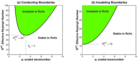
Figure 1: Critical Rayleigh number as a function of scaled horizontal wavelength $q$. (a) Conducting boundaries and (b)insulating (fixed-flux) boundaries.

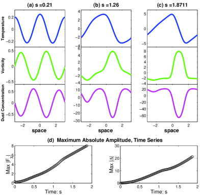
Figure 2: Representative profiles for Model A: $\tilde{\beta}=\tilde{b}_{1}=0$ and $r_{2}=5.30$ and $\tilde{\phi}=10$. Plotted are the lowest order temperature amplitude $F$, the lowest order vorticity amplitude $F_{\chi}$, followed by the dust concentration, $\Delta$. Panel (a), at time $s\sim 0.21$. Panel (b), time $s\sim 1.25$. Panel (c), blow up time $s\sim 1.87$. The scaled dust concentration always seems to trace the gas vorticity $F_{\chi}$ even throughout the blow up time. Panel (d) is the time series for the absolute values of vorticity scale and dust concentration, respectively.

3 An Asymptotic Nonlinear Model

In order to understand how to handle the curious situation involving the algebraic growth of the particle density perturbation even though the gas phase is neither growing nor decaying we asymptotically analyze the governing equations under certain extreme conditions. In particular, we will explore the nonlinear development of disturbances for fixed thermal flux boundary conditions. Furthermore we will assume that the Prandtl number is much larger than the scaled Coriolis parameter, $\tilde{f}$ which will also be much greater than one, viz.,

$$Pr\gg\tilde{f}\gg 1.$$

This extreme ordering says physically that the dust stopping time, $t_{s}$, is much longer than the local rotation time $\sim\Omega^{-1}$. This scaling however also says that the dust stopping time is much less than the geometric mean of the thermal and rotation times. In other words,

$$\frac{\tau}{\Omega}\gg t_{s}^{2},\qquad{\rm and}\qquad\Omega t_{s}\gg 1.$$

For the sake of this asymptotic calculation we take $Pr\rightarrow\infty$.

Furthermore we will suppose that the horizontal lengths scales are much larger than the scales in direction of gravity and we will introduce the small scaling parameter $\epsilon$ to represent this extreme state. Corresponding to this situation we introduce the scaled horizontal variable $X=\epsilon\xi$, where $X$ is an order one quantity. Additionally we introduce an order 1 scaled time variable $T$ such that $T=\epsilon^{4}t$. Thus, we replace all derivative operators with

$$\frac{\partial}{\partial\xi}\rightarrow\epsilon\partial_{X},\quad\frac{\partial}{\partial t}\rightarrow\epsilon^{4}\partial_{T}$$ (37)

From now on we will appeal to the shorthand notation for derivative operations for compactness of notation and clarity of derivation. Correspondingly, we find that a distinguished limit exists when the stream function is ${\cal O}\left({\epsilon}\right)$ the temperature fluctuation. Specifically, we say that

$$\tilde{\psi}=\epsilon\Psi,\qquad\tilde{\omega}=\epsilon\Omega,$$

where $\Psi$ and $\Omega$ are now order 1 quantities.

We introduce the external force, ${\cal F}_{k}$, into the analysis in which its nondimensionalization is expressed through the relationship,

$${\cal F}_{k}(y)=\frac{d}{\tau^{2}}\tilde{\cal F}_{k}(Y),$$

where $\tilde{\cal F}_{k}$ is nondimensional. We assume that the steady external force has the form

$$\tilde{\cal F}_{k}=\frac{1}{\epsilon^{4}}b\phi Y,$$ (38)

where $b$ and $\phi$ are order 1 constants.

In order to achieve proper asymptotic balance we exploit the freedom we have in choosing the “largeness” of the Coriolis parameter by scaling it (ad hoc) as

$$\tilde{f}=\frac{1}{\epsilon^{5}}\phi\left(1+\frac{\beta}{\phi}\epsilon^{6}Y\right)$$ (39)

where $\phi$ is, as before, order 1. The bizarre choice behind this asymptotic ordering is motivated by introducing the dust disturbance term $\tilde{\delta}$ into the subsequent analysis at the right stage. The $\beta Y$ term, which tacitly represents an assumption of a weak f-plane effect (see Pedlosky), is introduced a priori in order to ensure stability of the nonlinear model. Though it is an artificial device, it has the effect of causing a Rossby wave type of drift of a vortex pattern.

With respect to (15), the resulting steady x-direction flow is weakly Couette. Denoting the steady flow by $U$ and $U_{d}$ then we have

$$U=U_{d}=\epsilon bY+{\cal O}\left({\epsilon^{7}}\right).$$ (40)

From here on out, we consider disturbances of the dust and gas velocities on top and over this base state.

With these scalings in place we find that the dust quantities require the following scalings in order for there to be nontrivial balance: the fractional dust density scales as $\epsilon^{2}$ and from here on out it is written as

$$\frac{\rho^{\prime}_{d}}{\bar{\rho}_{d}}=\epsilon^{2}\delta.$$ (41)

We find that the dust dilatation is first nontrivial at order $\epsilon^{6}$ and it is written as,

$$\tilde{C}=\epsilon^{6}C_{6}+{\cal O}\left({\epsilon^{8}}\right)$$ (42)

whereas the dust vorticity scales even smaller such that it is nontrivial at order $\epsilon^{11}$! In other words,

$$\tilde{\omega}_{d}=\epsilon^{11}\Omega_{d}.$$ (43)

Because of this last observation we will, for all intents and purposes, treat the dust velocity as derived from a potential which similarly scales on order $\epsilon^{6}$. In other words, $u_{d}=\epsilon^{6}\nabla\Gamma$. As such, each component of the dust velocity scales as

$$\tilde{u}_{d}^{(y)}=\epsilon^{6}v_{6}=\epsilon^{6}\frac{\partial\Gamma}{\partial Y},\qquad\tilde{u}_{d}^{(x)}=\epsilon^{7}w_{7}=\epsilon^{7}\frac{\partial\Gamma}{\partial X}.$$ (44)

Together with the scaling relationship (42) and general definition (25) it is clear that at these initial orders the dust velocity satisfies a Poisson type of equation,

$$\nabla^{2}\Gamma=C_{6}.$$ (45)

With these scalings and assumptions in place we consider the temporal development of disturbances when the Rayleigh number deviates from its critical value by an order $\epsilon^{2}$ amount written as,

$$R\rightarrow R_{0}+\epsilon^{2}R_{2}.$$ (46)

For this analysis we will consider the development in terms of fixed-flux boundary conditions which means that the critical Rayleigh number about which we will be expanding around will be 12. However, the following calculation self-consistently selects the proper value of $R_{0}$. The governing equations (in the $Pr\rightarrow\infty$ limit) with these scalings inserted now reads for the gas phase,

$$R_{0}\left(1+\epsilon^{2}\frac{R_{2}}{R_{0}}\right)\partial_{X}\Theta-(1+\epsilon^{2}\delta_{2})\Omega = \epsilon^{2}\beta\partial_{X}\Psi$$ (47)

$$\epsilon^{4}\partial_{T}\Theta+\epsilon^{2}{\cal J}(\Theta,\Psi)+\epsilon^{2}b_{1}Y\partial_{X}\Theta = \epsilon^{2}\partial_{X}\Psi+\epsilon^{2}\partial_{X}^{2}\Theta+D^{2}\Theta$$ (48)

$$\Omega = \left(D^{2}+\epsilon^{2}\partial_{X}^{2}\right)\Psi,$$ (49)

and for the particle phase they are,

$$0 = \epsilon\Omega-\epsilon\phi C_{6}+{\cal O}\left({\epsilon^{7}}\right)$$ (50)

$$0 = -\epsilon^{6}C_{6}+\epsilon^{6}\phi\Omega_{d}+{\cal O}\left({\epsilon^{12}}\right)$$ (51)

$$\epsilon^{6}\partial_{T}\delta+\epsilon^{6}C_{6} = 0+{\cal O}\left({\epsilon^{8}}\right)$$ (52)

The new Jacobian symbol, ${\cal J}$ is defined on the variables $X$ and $Y$. In the next section we set out to solve, order by order, the set of equations (47-52) with fixed flux thermal boundary conditions.

3.1 Expansions

The set of equations (47-52) are solved as a perturbation series expansion in powers of $\epsilon^{2}$. Thus, the following expansions are presumed for this purpose,

$$\Theta=\Theta_{0}+\epsilon^{2}\Theta_{2}+\epsilon^{4}\Theta_{4}+\cdots$$ (53)

$$\Psi=\Psi_{0}+\epsilon^{2}\Psi_{2}+\cdots$$ (54)

$$\Omega=\Omega_{0}+\epsilon^{2}\Omega_{2}+\cdots$$ (55)

$$\delta=\delta_{2}+\epsilon^{2}\delta_{4}+\cdots$$ (56)

(48) to lowest order becomes simply,

$$D^{2}\Theta_{0}=0.$$ (57)

The solution of this equation subject to the condition that the flux remain fixed on the boundary is,

$$\Theta_{0}=f(X,T),$$ (58)

meaning to say that the lowest order temperature perturbation is independent of the vertical coordinate. The rest of the expansion procedure is standard and we relegate its full exposition to Appendix A. What results are two coupled evolution equations for the temperature disturbance $f$ and the lowest order particle density $\delta_{2}$ in (87) and (96). These are reproduced below,

$$f_{T} = -\kappa f_{XXXX}+\mu(f^{3}_{X})_{X}-\left[(r_{2}-\delta_{2})f_{X}\right]_{X}$$ (59)

$$-b_{1}S(f_{X}^{2})_{X}-\beta Bf_{XXX},$$

$$\delta_{2T} = -\phi R_{0}f_{X}.$$ (60)

The positive constants $\kappa,\mu,B,S$ are defined in Appendix A. $r_{2}$ is an effective departure from the critical Rayleigh number $R_{0}=12$ given by

$$r_{2}=\frac{R_{2}}{12}-\frac{b_{1}^{2}}{120}.$$

The parameter $r_{2}$ can be interpreted as representing an effective departure from criticality which includes the fact that a constant (linear) shear is a stabilizing influence against the onset of rolls in the linear regime.

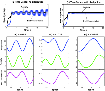
Figure 3: Representative profiles for Model B: $\tilde{b}_{1}=0$ and $r_{2}=5.30$, $\tilde{\phi}=10$, $\tilde{\beta}=-10$. (a), maximum amplitude of the dust concentration and the scaled vorticity when there is dissipation (${\cal B}=0$). The amplitudes oscillate with growing size on a long-time scale. (b), maximum amplitude of the dust concentration and the scaled vorticity with dissipation present, (${\cal B}=1$). The oscillations are quelled while the overall average maximum amplitude of the structures are preserved. Panels (c-e) representing profiles of $F,F_{\chi},\Delta$ at various stages in the ensuing evolution. It should be observed that the dust concentration, $\Delta$, eventually locks onto the temperature profile, $F$, at late times.

3.2 Canonization and Identification of Effects

It is more convenient to define a number of rescalings of (59) and (60) in order to transparently display the structure of the two coupled equations. One may define new space and time coordinates, $\xi$ and $s$ along with new amplitude scalings $F$ and $\Delta$ by,

$$T\rightarrow s\kappa,\qquad X\rightarrow\sqrt{\kappa}\chi,$$

$$f(X,T)\rightarrow\left(\frac{\kappa}{\mu}\right)^{1/2}F(\chi,s),\qquad\delta_{2}(X,T)\rightarrow\Delta(\chi,s).$$ (61)

Consequently, (59) and (60) rewritten in terms of the definitions (61) is

$$F_{s} = -F_{\chi\chi\chi\chi}+(F_{\chi}^{3})_{\chi}-\Bigl{(}(r_{2}-\Delta)F_{\chi}\Bigr{)}_{\chi}$$ (62)

$$\ \ \ \ -\tilde{b}_{1}(F_{\chi}^{2})_{\chi}-\tilde{\beta}F_{\chi\chi\chi},$$

$$\Delta_{s} = -\tilde{\phi}F_{\chi},,$$ (63)

where

$$\tilde{b}_{1}\equiv b_{1}\frac{S}{\mu},\qquad\tilde{\beta}\equiv\beta\frac{B}{\sqrt{\kappa}},\qquad\tilde{\phi}\equiv\phi R_{0}\frac{\kappa}{\sqrt{\mu}}.$$

The model set (62) and (63) are now in a more transparent form and allows us to discuss the effects they contain. The role of the first two terms on the RHS of (62) are well known (see Chapman & Proctor, 1980) respectively, (i) to damp the temperature profile due to horizontal thermal dissipation and (ii) to control amplitude due to nonlinear advection of temperature. The $r_{2}$ expression in the third term on the RHS of (62) constitutes the usual source of amplitude growth because of positive departures from the critical Rayleigh number. The $\Delta$ term expresses the fact that as the particle concentration grows the local Rayleigh number of the fluid goes down somewhat. This is best seen by observing the definition of the Rayleigh number (26): if the dust density $\rho_{d}$ goes up then $R$ goes down and vice versa. The other terms on the RHS of (62) represent, respectively, (iii) the nonlinear twisting of the temperature profile due to shear and (iv) an effective Rossby wave type of drift of an emerging profile. As discussed in the previous section, (63) represents the local enhancement of dust concentration due to the emerging convection roll’s vorticity, which is, to lowest order, proportional to $F_{\chi}$ as demonstrated in Appendix A.

Note that the nonlinear term $(F_{\chi}^{2})_{\chi}$ associated with the shear is known to promote subcritical transitions in Rayleigh-Benard convection (Gertsberg & Sivashinsky, 1981) and will do so here in this model as well but we will not explore this feature in this study. This term appears generically so long as there is some sort of symmetry-breaking effect in the system (e.g. see Depassier & Spiegel, 1982).

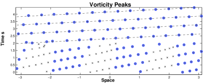
Figure 4: Position of the peaks of the vorticity profile for Model B. The maximum peak is labelled with a circle and all secondary peaks are denoted with x’s. After the transient readjustment phase is over (near $s\sim 2$) the system goes from multiple peaks to only one. After this time, the path of the peak is traced out with a dashed line and it is evident that it propagates from left to right on this spacetime diagram.

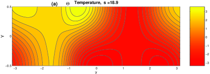
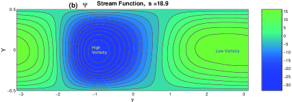
Figure 5: Representative contours for Model B when the growth has settled onto the steady state. For these contours $\epsilon=1$. (a) Temperature fluctuation contours, $\Theta$. (b) Stream function contours, $\Psi$.

3.3 Selected Solutions

The reduced asymptotic equations (62-63) are evolved according to the numerical spectral scheme outlined in Appendix B and is similar to the tactics used in Umurhan & Regev (2004). The robustness of the scheme was checked against the analytic solutions of a similar evolution equation derived by Chapman and Proctor (1980). The tests demonstrated agreement between the numerical scheme and the analytical results to one part in $10^{-7}$. The results reported here were generally computed on 256 Fourier modes and when convergence was doubted, the results were checked against simulations based on 512 and 1024 modes. Because there are fourth order derivatives in the linear terms of (62) we note that, (a) no artificial viscosity was needed and, (b) small time steps on the order of $dt=10^{-4}$ were typically taken. All simulations started out with random white noise for $F$ whose total amplitude did not exceed $10^{-2}$. The dust concentration always started out with zero initial amplitude.

We consider here four selected models to discuss;

• Model A. No background vorticity gradient and no shear, $\tilde{b}_{2}=\tilde{\beta}=0$, while $r_{2}=5.3$ and the dust coupling is set $\tilde{\phi}=10$,

• Model B. The background vorticity gradient is negative,$\tilde{\beta}=-10$, there is no shear $\tilde{b}_{2}=0$, along with $r_{2}=5.3$ and $\tilde{\phi}=10$ and,

• Model C Some amount of shear with a prograde sense, $\tilde{b}_{1}=-10.0$ along with the same values of $r_{2}$,$\tilde{\phi}$ and $\tilde{\beta}$ of Model B.

It should be noted that in all models the background vorticity is getting smaller with increasing $Y$. Additionally, the results reported here required there to be some dissipation added to the equation describing the dust concentration evolution or otherwise the solutions blow up. This is discussed in more detail for Model B.

3.3.1 Model A

This and other models like it, where $\tilde{\beta}=0$, are unstable. The amplitude and dust concentration steadily runaway once the dust concentration locks into the standing vorticity profile that emerges. To see this more readily refer to Figure 2. At early times in the simulation the local dust concentration grows fastest wherever $G=F_{\chi}$, which is proportional to the leading order vorticity, is greatest. This behavior is in line with the conclusions of the linear theory section. For $r_{2}=5.3$ and $\tilde{\phi}=0$ , the fastest growing wavenumber is $n=2$ and this readily shown in the linear theory analysis of (62). Despite the linear theory expectations however, the final roll profile will go from being double humped to being single humped as was shown by Chapman and Proctor (1980). This is because the nonlinear stability analysis shows that the system prefers to eventually settle onto a profile with a single roll.

With $\tilde{\phi}$ non-zero, the same sort of late time behavior is observed. The dust concentration also qualitatively resembles the vorticity distribution and it, similarly to the linear theory, appears to grow/deplete without bound. Those places where the vorticity amplitude is greatest are those places where the dust concentration is greatly depleted. Consequently, those locations in the gas correspond to greatly enhanced values of the local Rayleigh number thereby causing the roll profile there to continue growing, in what appears to be, without bound. Naturally, the validity of this predicted blowup should be questioned since unbounded growth means the asymptotic solution has ceased being valid.

3.3.2 Model B: Vorticity Gradient with No Shear

Introduction of $\tilde{\beta}$ stabilizes the runaway growth seen in Model A. The amplitude of the emerging convection roll settles onto the vicinity of a given value though on oscillation sets in. On a very long time scale this oscillation, which shows up in both the roll amplitude and dust concentration amplitude, exhibits a growth in amplitude and it eventually blows up as is evidenced in Figure 3a. This happens for all models in which $\tilde{\phi}$ is not zero and the secular growth time scale is shorter as $\tilde{\phi}$ becomes larger. In order to stabilize the long time behavior a dissipation term is introduced into the dust evolution equation so that, and from here on out, instead of (63) the following equation is evolved,

$$\Delta_{s}=-\tilde{\phi}F_{\chi}+{\cal B}\Delta_{\chi\chi},$$ (64)

${\cal B}$ is the scale of the dissipation and in the simulations it is taken to be unity. With the simulation run with ${\cal B}=1$, the resulting maximum absolute amplitude is shown in Figure 3b. The oscillations observed for ${\cal B}=0$ are removed and the overall average amplitude of the underlying structures are preserved.

The time evolution of these simulations begin with an initial growth phase. For $r_{2}=5.3$, the linear theory predicts that the fastest growing Fourier mode is $k=2$ and, as such, in the early stages the temperature profile is double humped as in Figure 3b. As Chapman and Proctor (1980) demonstrated, this type of profile is nonlinearly unstable and eventually the system undergoes a phase of transient readjustment (around $s=1.5$) in which the temperature and vorticity go from being a two-humped profile down to a one-humped profile. Figure 3c shows the state of this profile readjustment near the time $s\sim 1.7$.

Additionally, Figure 4 demonstrates how the profile drifts with increasing $\chi$ as a function of time. In this steady drifting state, the profiles are single humped and, as in Figure 3d, after the post readjustment phase the dust concentration profile locks onto the temperture profile tightly. The reason that the dust concentration does not grow without bound when the roll pattern drifts is simple. In Model A, because $\tilde{\beta}=0$, the temperature and vorticity profile that develops does so in place. Because the dust concentration responds to local variations of the vorticity, places in the growing roll profile where the vorticity is most reduced are also where the rate of dust collection is greatest. Without a suitable saturation mechanism the greatly enhanced dust concentration begins to modify the local Rayleigh number of the fluid. This, in turn, causes the roll amplitude to grow with ferocity. With a larger amplitude in the vorticity will come an ever increased concentration of dust. In this way the cycle feeds on itself and it runs away. On the other hand, when the roll profile drifts, local enhancements of dust do not grow without bound because the low vorticity patch of the fluid that causes the dust to concentrate will eventually drift past. The local dust will then encounter gas with a higher than normal degree of vorticity and this will cause the the dust concentration to begin to diminish.

Finally, Figures 5(a-b) show the temperature and stream function in the full 2D domain.

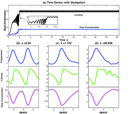
Figure 6: Representative profiles for Model C showing a prograde shear profile: $r_{2}=5.30$ and $\tilde{\phi}=10$, $\tilde{\beta}=-10$ along with $\tilde{b}_{1}=-10$. These results were generated with ${\cal B}=1$. (a) Time series of the absolute amplitude of $F_{\chi}$ and $\Delta$. The amplitudes reach a steady average value but each profile experiences a small amplitude oscillation that neither grows nor decays with time. Inset is shown a higher resolution profile of the transient phase for the vorticity near $s\sim 2$. The profile goes from nominally two large scale humps to one. Panels (b-d) show profiles of various quantities at three different times: (b), initial growth phase, time $s\sim 0.84$, (c), transient adjustment phase, time $s\sim 1.72$, (d), steady state phase, time $s\sim 20.0$. In (d) it is clear that the vorticity takes on significant and complicated structure and it is also apparent that those regions where the vorticity is negative are strongly concentrated.

3.3.3 Model C: Prograde Shear

Shear does not change the basic features of the results found for Model B. However, it does alter the appearence of the finally developed convection roll by giving it a much more complicated structure. As before, the evolution goes through an initial growth stage followed by a transient readjustment phase before settling onto a roughly steady profile (Figure 6a). The great difference between these results and that of Model B is that the negative vorticity of the roll is strongly concentrated into a small region in space whereas the positive vorticity, including all the substructures like in Figure 6d, are spread out over larger areas of space (Figure 7b).

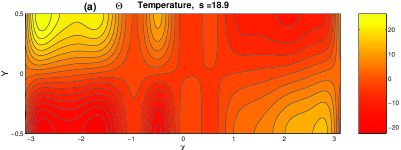
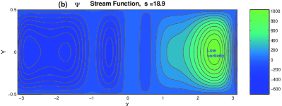
Figure 7: Representative contours for Model c in the quasi-steady state regime, $s\sim 18.9$. For these contour calculations, $\epsilon=1$. (a) Temperature fluctuation contours, $\Theta$. (b) Stream function contours, $\Psi$.

Appendix A Asymptotic Expansions

At infinite Prandtl numbers, the full governing equations (47-52) are reproduced here in slightly different form and with a little bit more detail,

$$R_{0}\left(1+\epsilon^{2}\frac{R_{2}}{R_{0}}\right)\partial_{X}\Theta-(1+\epsilon^{2}\delta)\Omega = \epsilon^{2}\beta\partial_{X}\Psi$$ (65)

$$\epsilon^{4}\partial_{T}\Theta+\epsilon^{2}{\cal J}(\Theta,\Psi)+\epsilon b_{1}z\partial_{X}\Theta = \epsilon^{2}\partial_{X}\Psi+\epsilon^{2}\partial_{X}^{2}\Theta+D^{2}\Theta$$ (66)

$$\Omega = \left(D^{2}+\epsilon^{2}\partial_{X}^{2}\right)\Psi$$ (67)

$$\epsilon^{6}C_{6} = \epsilon^{6}\phi\Omega+\cdots$$ (68)

$$\Omega_{d} = \epsilon^{11}\frac{1}{\phi}\Omega$$ (69)

$$\epsilon^{6}\partial_{T}\delta+\epsilon^{6}(1+\epsilon^{2}\delta)C_{6} = -\epsilon^{3}u^{(x)}_{d}\partial_{X}\delta-\epsilon^{2}u^{(y)}_{d}D\delta$$ (70)

The following expansions are presumed

$$\Theta=\Theta_{0}+\epsilon^{2}\Theta_{2}+\epsilon^{4}\Theta_{4}+\cdots$$ (71)

$$\Psi=\Psi_{0}+\epsilon^{2}\Psi_{2}+\cdots$$ (72)

$$\Omega=\Omega_{0}+\epsilon^{2}\Omega_{2}+\cdots$$ (73)

$$\delta=\delta_{2}+\cdots$$ (74)

and similarly for the other quantities. At the lowest order (66) is,

$$D^{2}\Theta_{0}=0$$ (75)

which admits the solution $\Theta_{0}=f(X,T)$. Next solve the next order momentum equation (65) and stream function relationship (67)

$$R_{0}\partial_{X}\Theta_{0}-\Omega_{0}=0,\qquad\Omega_{0}=D^{2}\Psi_{0},$$ (76)

together these equations yield the solution

$$\Psi_{0}=R_{0}P_{0}f_{X},\qquad P_{0}=\frac{y^{2}}{2}-\frac{1}{8},$$ (77)

where $P_{0}$ is designed so that there is no normal flow of fluid at the vertical boundaries, or in other words, $\Psi_{0}=0$ at $y=\pm 1/2$. We note that because of the relationships between the lowest order vorticity, stream function and the temperature in (76) and (77), the vorticity is proportional to the gradient of the temperature structure function, or in other words, $\Omega_{0}\sim F_{X}$.

In order for a solution to exist for the temperature at the next order, a solvability condition must be enforced upon the equations at this order. This means that starting with,

$$D^{2}\Theta_{2}=-\partial_{X}\Psi_{0}-\partial_{X}^{2}\Theta_{0}+b_{1}y\partial_{X}\Theta_{0}+\partial_{X}(\Psi_{0})D\Theta_{0}-D(\Psi_{0})\partial_{X}\Theta_{0},$$ (78)

the solvability condition, in which the thermal flux at the vertical boundaries is fixed, amounts to requiring,

$$\int_{-1/2}^{1/2}D^{2}\Theta_{2}dy=D\Theta_{2}|^{y=1/2}_{y=-1/2}=0.$$ (79)

Since $\Theta_{0}$ is constant with respect to $y$ and since $\Psi_{0}$ is an even function of $y$, we find that the condition (79) applied to (78) results in a choice for $R_{0}$,

$$1+R_{0}\int_{-1/2}^{1/2}P_{0}dy=0.$$ (80)

From (77), it follows that $R_{0}=12$. The solution of $\Theta_{2}$ becomes

$$\Theta_{2}=T_{2}f_{XX}+M_{2}(f_{X})^{2}+b_{1}N_{2}f_{X},$$ (81)

where the individual functions, $T_{2},M_{2},N_{2}$ are given by

$$D^{2}T_{2}=-1-R_{0}P_{0}, T_{2}=\frac{y^{2}}{4}-\frac{y^{4}}{2},$$ (82)

$$D^{2}M_{2}=-R_{0}DP_{0}, M_{2}=\frac{3y}{2}-2y^{3},$$ (83)

$$D^{2}N_{2}=z, N_{2}=-\frac{y}{8}+\frac{y^{3}}{6}.$$ (84)

these are also designed so their y-derivatives are zero at the boundaries $y=\pm 1/2$. Because $u^{(x)}_{d}$ and $u^{(y)}_{d}$ are order $\epsilon^{7}$ and $\epsilon^{6}$ respectively, and furthermore, because of the relationship between the particle divergence and the gas vorticity in (68), the lowest order expression of (70) is

$$\partial_{T}\delta_{2}+\phi\Omega_{0}=0.$$ (85)

But because of the solutions (76) and (77) we may write

$$\delta_{2}=\delta_{2}(X,T),$$ (86)

in other words, the structure function $\delta$ for the particle concentration is independent of $y$ at this order. The governing evolution equation for $\delta_{2}$ is rewritten to reflect the solution $\Omega_{0}$,

$$\partial_{T}\delta_{2}=-\phi R_{0}f_{X}.$$ (87)

We may now proceed to order $\epsilon^{2}$ and solve for the next order stream function $\Psi_{2}$. The governing equation becomes,

$$D^{2}\Psi_{2}=R_{0}\partial_{X}\Theta_{2}+R_{2}\partial_{X}\Theta_{0}-\partial_{X}^{2}\Psi_{0}-\delta_{2}\Omega_{0}-\beta\partial_{X}\Psi_{0}$$ (88)

Utilizing the solutions from the previous orders we find that the $\Psi_{2}$ may be written as

$$\Psi_{2} = S_{2}f_{XXX}+(R_{2}-\delta_{2}R_{0})P_{0}f_{X}+Q_{2}\partial_{X}(f_{X})^{2}$$ (89)

$$+\left(b_{1}L^{({\rm odd})}_{2}-\beta L^{({\rm even})}_{2}\right)f_{XX}$$

where the structure functions appearing above are given by

$$D^{2}S_{2}=R_{0}T_{2}-R_{0}P_{0}, S_{2}=-\frac{y^{6}}{5}-\frac{y^{4}}{4}+\frac{3y^{2}}{4}-\frac{27}{160},$$ (90)

$$D^{2}Q_{2}=R_{0}M_{2}, Q_{2}=-\frac{6y^{5}}{5}+3y^{3}-\frac{27y}{40},$$ (91)

$$D^{2}L^{({\rm odd})}_{2}=R_{0}N_{2}, L^{({\rm odd})}_{2}=\frac{y^{5}}{10}-\frac{y^{3}}{4}+\frac{9y}{160},$$ (92)

$$D^{2}L^{({\rm even})}_{2}=R_{0}P_{0}, L^{({\rm even})}_{2}=\frac{y^{4}}{2}-\frac{y^{2}}{4}+\frac{5}{32}.$$ (93)

The structure functions are designed so that they are zero at the boundaries $y=\pm 1/2$. Next we turn to the order $\epsilon^{4}$ heat equation which is,

$$\partial_{T}\Theta_{0}+{\cal J}(\Psi_{2},\Theta_{0})+{\cal J}(\Psi_{0},\Theta_{2})+b_{1}y\partial_{X}\Theta_{2}=$$

$$\ \ \ \ \partial_{X}\Psi_{2}+\partial_{X}^{2}\Theta_{2}+D^{2}\Theta_{4}.$$ (94)

Like at the previous order the solvability condition is,

$$\int_{-1/2}^{1/2}D^{2}\Theta_{4}dy=D\Theta_{4}|^{y=1/2}_{y=-1/2}=0.$$ (95)

The solvability condition produces an evolution equation for $f$, namely,

$$f_{T}+\kappa f_{XXXX}-\mu(f^{3}_{X})_{X}$$

$$+\left[(r_{2}-\delta_{2})f_{X}\right]_{X}+b_{1}S(f_{X}^{2})_{X}+\beta Bf_{XXX}=0,$$ (96)

where the constants and parameters are defined by,

$$\kappa = -\int^{1/2}_{-1/2}(S_{2}+T_{2})dy=\frac{2}{21},$$ (97)

$$\mu = -R_{0}\int^{1/2}_{-1/2}(P_{0}DM_{2})dy=\frac{6}{5},$$ (98)

$$r_{2} = -R_{2}\int^{1/2}_{-1/2}Pdy+b_{1}^{2}\int^{1/2}_{-1/2}zN_{2}dy=\frac{R_{2}}{R_{0}}-\frac{b_{1}^{2}}{120},$$ (99)

$$S = R_{0}\int^{1/2}_{-1/2}P_{0}DN_{2}dy=\frac{1}{10},$$ (100)

$$B = R_{0}\int^{1/2}_{-1/2}L^{({\rm even})}_{2}dy=\frac{1}{10}.$$ (101)

Appendix B Numerical Method

The general form of the equations we seek to solve are,

$$\frac{\partial F}{\partial s} = {\cal L}F+{\cal N}(F,\Delta)$$ (102)

$$\frac{\partial\Delta}{\partial s} = {\cal M}(F),$$ (103)

where ${\cal L}$ is some linear operator and where ${\cal N}$ is a nonlinear operator involving some combination of the arguments and ${\cal M}$ is linear in $F$.

These one dimensional equations will be solved in terms of Fourier expansions of $F$ and $\Delta$ as in,

$$F = \sum F_{k}(s)\exp{ik\chi}+{\rm c.c.}$$ (104)

$$\Delta = \sum\Delta_{k}(s)\exp{ik\chi}+{\rm c.c.},$$ (105)

such that each Fourier component evolves according to

$$\frac{\partial F_{k}}{\partial s} = {\cal L}_{k}F_{k}+{\cal N}_{k}(F,\Delta)$$ (106)

$$\frac{\partial\Delta_{k}}{\partial s} = {\cal M}_{k}(F).$$ (107)

The scalars ${\cal L}_{k}$ are the linear operator ${\cal L}$ acting on the appropriate Fourier wave $k$ and where ${\cal N}_{k}$ and ${\cal M}_{k}$ are the $k$th components of each respective operator ${\cal N}$ and ${\cal M}$.

The symbol $F^{n}$ represents the nth time iterate of $F$. This same convention carries over to $\Delta$, ${\cal M}$ and ${\cal N}$ . The evolution is carried out using a second order time centered difference scheme together with a Crank-Nicholson scheme for the spatial wavenumbers of the linear operator terms. All ${\cal N}_{k}$ and ${\cal M}_{k}$ expressions are evaluated at the centered time point. With $\delta s$ as the time increment between time step $n$ and $n+1$ the discretized equations are,

$$\frac{F^{n+1}_{k}-F^{n-1}_{k}}{2\delta s} = \frac{{\cal L}_{k}F^{n+1}_{k}+{\cal L}_{k}F^{n-1}_{k}}{2}+{\cal N}^{n}_{k},$$ (108)

$$\frac{\Delta^{n+1}_{k}-\Delta^{n-1}_{k}}{\delta s} = {\cal M}^{n}_{k}.$$ (109)

Rearranging the terms and isolating the $n+1$ time step reveals,

$$F^{n+1}_{k} = \frac{1+\delta s{\cal L}_{k}}{1-\delta s{\cal L}_{k}}F^{n-1}_{k}+\frac{2\delta s}{1-\delta s{\cal L}_{k}}{\cal N}^{n}_{k},$$ (110)

$$\Delta^{n+1}_{k} = \Delta^{n-1}_{k}+2\delta s{\cal M}^{n}_{k}.$$ (111)

In the first discretization above, the coefficient terms in front of $F^{n-1}_{k}$ and ${\cal N}^{n}_{k}$ look like Páde approximants to exponentials of ${\cal L}_{k}$. This is then assumed and the following replacements,

$$\frac{1+\delta s{\cal L}_{k}}{1-\delta s{\cal L}_{k}}\rightarrow\exp\left[2\delta s{\cal L}_{k}\right],\qquad\frac{1}{1-\delta s{\cal L}_{k}}\rightarrow\exp\left[\delta s{\cal L}_{k}\right],$$ (112)

are made in (110). The resulting discretized equations that are simultaneously solved at each time step are (111) along with,

$$F^{n+1}_{k}=\exp\left[2\delta s{\cal L}_{k}\right]F^{n-1}_{k}+2\delta s\exp\left[\delta s{\cal L}_{k}\right]{\cal N}^{n}_{k}.$$ (113)

Time centered differenced schemes like the simple one used here are known to sometimes incur a period $2\delta s$ long-time numerical instability. In order to wash this effect out, at every 50th timestep (113) and (111) are advanced through for one time step using an Euler type evolver as in the following,

$$F^{n+1}_{k} = \exp\left[\delta s{\cal L}_{k}\right]F^{n}_{k}+\delta s\exp\left[\delta s{\cal L}_{k}\right]{\cal N}^{n}_{k},$$ (114)

$$\Delta^{n+1}_{k} = \Delta^{n}_{k}+\delta s{\cal M}^{n}_{k}.$$ (115)

This Euler advancer is also used as the very first time step of all simulations.

References

- [1995] Barge P. & Sommeria, J., 1995, A&A, 295, L1.
- [2000] Barranco J.A. & Marcus, P.S., 2000, Summer Program Proceedings, Center For Turbulence Research, NASA Ames/Stanford Univ. 97.
- [2005] Barranco J.A. & Marcus, P.S., 2005, ApJ, 623, 1157.
- [2006] Bertin, G. & Cava, A., 2006, A&A, 459, 333.
- [1999] Bracco, A., Chavanis P.H., Provenzale, A. & Spiegel E.A., 1999, Phys. of Fluids,11, 2280.
- [1954] Chandresekhar, S., 1954, Proc. Roy. Soc. (London) A, 225, 173.
- [1980] Chapman, C. J. & Proctor, M. R. E., 1980, J. Fluid Mech., 101, 759.
- [1997] Chiang, E.I. & Goldreich, P., 1997, ApJ, 490,368.
- [1993] Cuzzi, J.N. Dobrovolskis, A.R. & Champney, J.M., 1993, 106, 102.
- [1982] Depassier, M.C. & Spiegel, E.A., 1982, Geophys. Astrophys. Fluid Dynamics, 21,167.
- [1981] Gertsberg, V. L. & Sivashinsky, G. I., 1981, Prog. Mod. Phys., 66, 1219.
- [1981] Hayashi, C., 1981, Prog. Theor. Phys. Suppl., 70, 35.
- [1945] Horton, C.W. & Rogers F.T., 1945, J. Appl. Phys., 16, 367.
- [2003] Klahr, H.H and Bodenheimer, P., 2003, ApJ, 582, 869.
- [1987] Pedlosky, J., 1987, Geophysical Fluid Dynamics: Second Edition, Springer-Verlag, New York.
- [1991] Squires, K.D. & Eaton J.K., 1991, Phys. Fluids A, 3, 1169.
- [1996] Tanga, P., Babiano, A, B. Dubrulle & Provenzale, A., 1996, Icarus, 121, 158.
- [2004] Umurhan, O.M. & Regev O., 2004, A&A, 427, 855.
- [2005] Youdin, A. & Goodman, J., 2005, ApJ, 620, 459.