The mass and luminosity functions and the formation rate of DA white dwarfs in the Sloan Digital Sky Survey

Abstract

Aims. The SDSS Data Release 1 includes 1833 DA white dwarfs (WDs) and forms the largest homogeneous sample of WDs. This sample provides the best opportunity to study the statistical properties of WDs.

Methods. We adopt a recently established theoretical model to calculate the mass and distance of each WD using the observational data. Then we adopt a bin-correction method to correct for selection effects and use the $1/V$ weight-factor method to calculate the luminosity function, the continuous mass function and the formation rate of these WDs.

Results. The SDSS DA WD sample is incomplete and suffers seriously from selection effects. After corrections for the selection effects, only 531 WDs remain. From this final sample we derive the most up-to-date luminosity function and mass function, in which we find a broad peak of WD masses centered around 0.58$M_{\odot}$. The DA WD space density is calculated as $8.81\times 10^{-5}pc^{-3}$ and the formation rate is $2.579\times 10^{-13}pc^{-3}yr^{-1}$.

Conclusions. The statistical properties of the SDSS DA WD sample are generally in good agreement with previous observational and theoretical studies, and provide us information on the formation and evolution of WDs. However, a larger and more complete all-sky WD sample is still needed to explain some subtle disagreements and unresolved issues.

1 Introduction

Studies of white dwarfs (WDs) have developed substantially in the last century. Chandrasekhar (1933, 1939) first developed a theoretical WD model by applying Fermi-Dirac statistics of electron and predicted a relationship between the mass and radius (M–R relation) of the WD. Hamada & Salpeter (1961) improved the model for the zero-temperature degenerate configuration by incorporating the assumption of various cores (H, He, C, O, Si, Mg, Fe) for different WDs. Wood (1990, 1995) considered more details such as the finite-temperature effect on the radius and the envelope of WDs, and derived theoretical models by calculating the stellar evolution. These models were widely employed in the following decade. Two of the latest model calculations are those of Panei et al (2000) and Fontaine et al. (2001). On the observational side, thousands of WDs have been detected in large sky surveys, such as those of the Extreme Ultraviolet Explorer (EUVE), the Palomar–Green Surveys (PG), ROSAT All-sky Survey, 2DF QSO Survey and the Sloan Digital Sky Survey (SDSS). Various spectral and photometric parameters of these WDs have been obtained. McCook & Sion (1999) published a catalog including 2245 spectroscopically identified WDs. The SDSS Data Release 1 (DR1) included 2551 identified WDs (Kleinman et al. 2004), of which only a few WDs were already in the catalog of McCook & Sion (1999). The Hipparcos data (Schmidt 1996; Provencal et al. 1998) provided a reliable source of the proper motions and parallaxes of a few WDs. The orbital parameters of WDs in visual binaries (e.g. radial velocities of WDs in common proper motion (CPM) systems) can also be obtained from observations (see e.g. Thorstensen et al. 1978, Vennes et al. 1999, Wegner & Reid 1987, Wegner et al. 1989).

The effective temperature $T_{eff}$ and surface gravity $log\ g$ can be derived from fitting the Balmer line profiles of WDs. Detailed discussions about the fitting techniques can be found in Bergeron, Saffer & Liebert (1992, hereafter BSL) and references therein. $T_{eff}$ can also be derived from the photometric colors by using an atmosphere model. To test the theoretical M–R relation, we need to estimate the mass and radius of WDs by directly measuring the flux, distance and the gravitational redshift of them. The distance of a nearby WD can be obtained directly from the measured parallax. The gravitational redshifts of some WDs in the CPM systems have been measured (see Wegner & Reid 1987; Wegner et al. 1989). However, these direct measurements can be done only for a few WDs.

Calculating the mass of WDs from the fundamental parameters mentioned above (such as $T_{eff}$ and $log\ g$) is the key to obtain the mass distribution of a large WD sample. Currently there are four kinds of methods to determinate the WD mass (see section 3 for details). There are a number of previous determination of WD masses (Koester, Schulz & Weidemann 1979, Weidemann & Koester 1984, McMahan 1989, Weidemann 1990, BSL, Finley et al. 1997, Marsh et al. 1997a, b, Vennes et al. 1997, Vennes 1999, Napiwotzki et al. 1999, Madej et al. 2004; Liebert et al. 2005). All of these obtained the mass distribution based on the spectroscopic WD masses, while BSL, Bergeron, Liebert & Fulbright (1995) and Reid (1996) obtained the mass distribution based on the gravitational redshifts. Although the gravitational redshift measurements are certainly important, these can be obtained only for a few WDs. For a large sample of WDs, estimating their masses from the spectroscopic data is probably the only possible way.

Generally, the mass distribution, the luminosity and mass functions (LF and MF) of the WDs can be constructed when the sample of WDs is large and complete enough. The luminosity function (LF) and the mass function (MF) derived from a sufficiently large sample of WDs in the solar neighborhood are very helpful for the study of the WD formation history. The LF reveals the current formation rate or death rate of stars in the local Galactic disk, and the MF can display the roles of close binary evolution in the WD formation process (Schmidt, 1959, 1963, 1968, 1975; Green 1980; Fleming et al. 1986; Liebert et al. 2005). In particular, Liebert et al. (2005) studied the mass distribution of a volume-limited sample, and obtained the luminosity and mass functions and the recent formation rate of DA WDs based on the 348 hot WDs from the PG survey.

The aim of the present paper is to derive the mass distribution and luminosity and mass functions of the large sample of DA WDs in the SDSS DR1, taking advantage of the larger volume of SDSS DR1 to obtain more reliable results. We have investigated the whole 1833 DA white dwarfs in the SDSS DR1, and calculated the mass, radius, bolometric magnitude, cooling age, and distance of these WDs using the recently published theoretical evolutionary models of Panei et al. (2000). These models cover a broader and denser parameter space than the models of Wood (1990, 1995), and are more able to be applied to obtain the spectroscopic masses for a large sample of WDs. Based on the derived parameters, we constructed the luminosity function, mass function and determined the formation rate of DA WDs. Due to the magnitude-limited selection effect of SDSS, the sample is far from the completeness needed to obtain statistically reliable results. Therefore, after introducing the sample and mass estimation method in section 2, we investigate the sample completeness and correct the selection effects in section 3. Then we study the luminosity function, mass function, formation rate and 3-dimensional distribution properties of DA WDs in sections 4 to 7. We briefly summarize and discuss our results in section 8.

2 The SDSS DA WD sample and the mass estimates with the evolutionary model

The SDSS is an ongoing imaging and spectroscopic survey of about ten thousand square degrees in the north Galactic cap to determine the brightness, positions, and obtain optical spectra of various objects (York et al. 2000). Although it mainly focuses on the extragalactic objects, there are many Galactic spin-off projects of which one is to acquire high-quality stellar spectra from stars of different spectral types. The spectroscopic survey in the SDSS DR1 covers a area of 1360 $deg^{2}$. Kleinman et al. (2004) published catalogs of the spectroscopic WD and hot subdwarf sample from the SDSS DR1 (Abazajian et al. 2003). They presented the spectral fitting results of 2551 certain WDs, 240 hot subdwarf stars and another 144 possible, but uncertain WDs and hot subdwarf stars. In this paper, we use the spectral data of 1833 DA WDs. Kleinman et al. (2004) derived the effective temperatures ranging from 7220K to 93855K, and the surface gravities $\log g$ from 6.25 to 9.00 (in $cgs$ units), using the pure hydrogen atmosphere model of Koester et al. (2001). The photometric parameters include the five magnitudes in $ugriz$ system (the magnitudes at g band being from 15.20 to 20.55), the proper motion velocity, the extinction index of g band and the value of signal to noise. The WD data of the SDSS DR1 are available at the SDSS website .

Previous studies (e.g. Clemens 1993; Barstow et al. 1993) provided evidence that a DA white dwarf most likely has a thick hydrogen layer of about $q(H)=-4$. In addition, the suggestion that most of high mass DA WDs have a C/O core and the low-mass DA WDs have a helium core has been widely accepted in former studies (e.g. Napiwotzki et al. 1999, Madej, Nalezyty & Althauset 2004, Liebert et al. 2005). Theoretical studies also show that when the mass of a WD is less than 0.45 $M_{\odot}$, the progenitors of these WDs could not reach high enough central temperatures for helium to be ignited at the center (Panei et al. 2000), providing further evidence for a helium core of low-mass DA WDs. BSL, Finley et al. (1997), Marsh et al. (1997a, 1997b), Vennes et al. (1997), Vennes (1999) and Liebert et al. (2005) all adopted Wood’s evolutionary model (Wood 1990, 1995) of a C/O-core with a thick hydrogen envelope in their studies. Madej et al. (2004) brought in the evolutionary models of Panei et al. (2000) assuming a C/O core with $M(H)/M=10^{-5}$ in the atmosphere of massive WDs and a helium core with $M(H)/M=3\times 10^{-4}$ for WDs with a mass less than 0.45 $M_{\odot}$. In this paper, we use the evolutionary helium-core model for WDs with mass less than 0.45 $M_{\odot}$ and bring in the C/O-core model for those with mass larger than 0.45 $M_{\odot}$. Both models are from Panei et al. (2000). In this paper we assume that all DA WDs (with either a C/O or helium core) have a thick hydrogen layer ($q(H)=-4$, $z=0.001$) for simplicity.

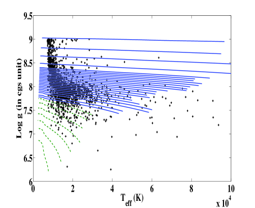
Figure 1: The $\log g$ - $T_{eff}$ diagram. The lines represent the theoretical results from the evolutionary model of Panei et al. (2000). The seven dashed lines at the bottom represent the results for the He-core WDs with a hydrogen layer. The solid lines represent the results for the C/O-core WDs with a hydrogen layer. These lines correspond to masses of (from bottom to top) 0.15, 0.2, 0.25, 0.3, 0.35, 0.4, 0.45 $M_{\odot}$ for He-core WDs, and 0.45, 0.47, 0.50, 0.52, 0.54, 0.56, 0.58, 0.60, 0.62, 0.64, 0.68, 0.70, 0.72, 0.74, 0.76, 0.78, 0.80, 0.82, 0.84, 0.90, 1.0, 1.10, 1.20 $M_{\odot}$ for C/O-core WDs respectively. The 1833 DA WDs of SDSS DR1 are plotted as crosses.

The predictions of the models of Panei et al. (2000) and the data ($\log g$, $T_{eff}$) of all DA non-magnetic WDs in the SDSS DR1 are plotted in Fig. 1. From it we can see that the models we chose are appropriate for our study. The predicted parameters of two models (He-core and C/O-core) cover a lager parameter range in the figure. The C/O models cover $T_{eff}$ from about 4000K to 100000K, and $log\ g$ from 7.43 to 9.03, while the He-core models cover $T_{eff}$ from 2500K to 27000K and $log\ g$ from 6.2 to 7.7. Most observed data of the DA WDs in the SDSS DR1 are within the range of these models. Some high temperature WDs at the right part of Fig. 1 are not covered by any models. The parameters of these extremely high-temperature WDs were discussed in BSL ( they limited the $T_{eff}$ of their WD sample to less than 40000K). There is a large discrepancy between the effective temperatures obtained from two different methods of fitting the Balmer lines when the $T_{eff}$ of a WD is above 50000K. We eliminate the WDs with extremely high $T_{eff}$ ($T_{eff}$ $>$ 48000K) from our samples. Because these WDs ( 39 objects) are only a very small fraction (about 2%) of the whole sample, their influence on the completeness of the sample is small.

To ensure that our calculation of WD parameters through the evolutionary model is reliable, we tested the model by comparing the WD masses derived from the evolutionary model and spectroscopic parameters ($T_{eff}$ and $\log g$) with the masses obtained from other independent methods. Currently there are three methods to determine the masses of WDs without involving the evolutionary models, namely:

(1) If a WD is in a binary system, we can precisely calculate the WD mass from its orbital parameters, but systems with complete spectroscopic parameters are relatively rare. Only a few WDs, including Sirius B (Gatewood & Gatewood 1978; BSL; Provencal et al. 1998; Barstow et al. 2005), 40 Eri B (Shipman et al. 1997; Wegner 1980; Finley et al. 1997), and Feige 24 (Vennes et al. 1991), have two independent estimates of their masses.

(2) If a WD does not have the orbital data, but has a parallax value from which the distance of it can be derived, we can obtain its absolute magnitude $M_{V}$ from $M_{V}=V+5+\log\pi$, where $V$ is the V band magnitude of the star and $\pi$ is the parallax in units of $arcsec$. Then we can obtain the bolometric magnitude from $M_{bol}=M_{V}+B.C._{V}$, where $B.C.$ is the bolometric correction in the $V$ band, which can be estimated by the interpolation of the grid of the atmosphere model (Bergeron et al. 1995b). Then from equations $M_{bol}=-2.5\log(L/L_{\odot})+M_{bol,\odot}$ and $L=4\pi R^{2}\sigma T_{eff}^{4}$ (here $\sigma$ is the Stephan-Boltzmann constant), the radius $R$ can be derived. By using Newton’s law of gravitation, we can obtain the mass of a WD.

(3) In some cases, the WD mass can be derived from the gravitational redshift $\Delta\lambda/\lambda$, which is usually described by the equivalent Doppler shift velocity: $v=c\frac{{\Delta\lambda}}{\lambda}=0.6362\frac{M}{{M_{\odot}}}\cdot\frac{{R_{\odot}}}{R}(km/s)$. So if we know the radius (or mass) from the second method mentioned above, we can easily derive the mass (or radius) accordingly.

In Table 1 we list the parameters and the references of the WDs which have both spectroscopic mass (derived from $T_{eff}$ and $\log g$ by using the evolutionary model of Panei et al. (2000)) and mass derived from one of the other three methods without using the evolutionary model. We note that BSL, Bergeron et al. (1995a), Provencal et al. (1998), and Boudreault & Bergeron (2005) have compared the masses of some WDs derived from different methods. Here we incorporate these WDs in Table 1 and re-estimate the spectroscopic masses of WDs using the new evolutionary model of Panei et al. (2000). We also add dozens of DA WDs that are not included in these previous studies.

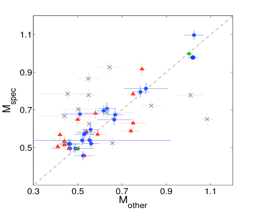
Figure 2: A comparison between the WD mass derived from the evolutionary model and those determined by other methods without using a theoretical M-R relation. Both axes are in unit of $M_{\odot}$. All points in the diagram are listed in Table 1. Triangles represent the WDs with mass determined by the triangle parallaxes and surface gravity. Circles represent WDs with mass determined by the gravitational redshifts. Squares represent WDs with mass derived from the orbital parameters. Crosses represents WDs cooler than 12000K. The dashed line represents $M_{spec}=M_{other}$.

Fig. 2 shows the comparisons of the WD masses obtained from different methods. WDs were divided into two groups, one with $T_{eff}$ less than 12000K (represented by crosses) and the other with $T_{eff}$ higher than 12000K. We can see that except for several WDs with $T_{eff}$ less than 12000K the masses estimated with different methods are in good agreement. For WDs with $T_{eff}$ less than 12000K, the differences in masses estimated by different methods are obviously larger. This is because these cooler WDs are likely to be convective. BSL have convincingly proved that the convection effect leads to significant amounts of helium (which is invisible in the spectra) entering the atmosphere, producing higher pressure which would substantially affect the spectral line profiles. The total effect on the spectral line is indistinguishable from the increased surface gravity. In other words, a low-temperature DA WD with large surface gravity might actually be a helium-rich star with lower surface gravity (and correspondingly with lower mass). So the scatter in the masses estimated with different methods for cooler WDs possibly has less to do with the evolutionary model that we adopted but is mainly due to the techniques of analyzing the spectral lines. For this reason, we remove these WDs from our statistical analyses.

There are still some high-temperature WDs for which the different mass estimates do not match very well. A few factors can contribute to this discrepancy, such as the techniques of fitting the spectral lines, the uncertainties of the observational parameters. etc. One of the most important factors is that there seems to be no appropriate evolutionary model for these high-temperature WDs. For example, G238-44, GD140, EG50, and EG21 have relatively higher spectroscopic mass compared with the mass derived from other methods. If we apply a thin hydrogen layer model ($q(H)=-1$, $q(He)=-4$) or a metal core (like $Fe$ core) for these four WDs, their spectroscopic mass will be lower by 0.04$\sim$0.06 $M_{\odot}$, and thus the mass comparison of these four WDs would be better. Moreover, the presence of helium in the atmosphere would also significantly influence the mass estimate. Boudreault & Bergeron (2005) gave a detailed discussion of this effect. They calculated the masses by using the models of Fontaine et al. (2001) and assuming a mixed composition in the atmosphere with $M(He)/M(H)=1$ rather than a pure hydrogen atmosphere, and obtained similar results that the mean $M_{spec}$ of WDs in their sample will be lower by 0.2 $M_{\odot}$. Thus, if we adjust the thickness of the envelope, the composition of the atmosphere and the atom in the core, more than half of the WDs in Fig. 2 will have their $M_{spec}$ equal to the mass derived by the other method. Therefore, we may find the most appropriate evolutionary model for each WD by matching two kinds of mass estimates, and then the discrepancy in Fig. 2 would be alleviated.

However, for most DA WDs from SDSS DR1 in our sample, we do not have parallax or gravitational redshift data to derive a second mass estimate and do not have further information about their internal structure and atmospheric composition. So we will just assume a theoretically appropriate model for our samples. From Fig. 2, we find that the comparison results are satisfactory in general, ignoring the low-temperature WDs. We then conclude that the assumptions of evolutionary models we adopted are generally reliable.

After testing the applicability of the model of Panei et al. (2000), we use it to calculate the masses of SDSS DA WDs in our sample. From the $T_{eff}$-$\log g$ diagram shown in Fig. 1, we can see that using the two parameters $T_{eff}$ and $\log g$ we can determine the mass of the WDs (the theoretical lines can be interpolated to cover the area that the lines do not cover in the figure). The other parameters of the WDs also can be calculated based on the mass estimation.

Using the methods described above, we can calculate the radius $R$, luminosity $L$ and bolometric magnitude $M_{bol}$ for WDs. Similar to the determination of mass, the cooling age of a WD can be derived by interpolating the grids of the evolutionary models, thus $\log Age=\log Age(T_{eff},\leavevmode\nobreak\ \log g)$. The bolometric correction ($B.C.$) in the g band can be obtained by using the model atmospheres of Bergeron et al. (1995b). $B.C.$ is derived through interpolating the $T_{eff}$ and $\log g$ into the grid of the model atmosphere in Bergeron et al. (1995b) for the $ugriz$ system, $B.C.=B.C._{Bergeron}(T_{eff},\log g)$. The distance $r$ (in $pc$) of the star can be derived from the $B.C.$ and the relationship between the absolute magnitude and visual magnitude in the g band: $M_{bol}=M_{g}+B.C._{g}$, $M_{g}=g-5-5\log{\rm{r}}-{\rm A}_{g}$, where $A_{g}$ is the extinction in the g band which is provided by the SDSS.

To compare our results with other previous work, we also derived the absolute magnitude of WDs in the V band which were commonly used in previous studies. Using the results of Bergeron et al. (1995b), we can easily convert the $M_{g}$ of the $ugriz$ system to the $M_{V}$ of the $UBV$ system. Bergeron et al. (1995b) provide the grids in both $ugriz$ and $UBV$ systems and the relationship between them, so we can obtain the bolometric correction in the $V$ band and $M_{V}$ of the $UBV$ system by interpolating the $T_{eff}$ and $\log g$ in the grid. Both $M_{V}$ and $B.C._{V}$ (bolometric correction at V band) are a function of $T_{eff}$ and $log\ g$, namely, $B.C._{V}=B.C._{V,Bergeron}(T_{eff},\log g)$, and $M_{V}=M_{V,Bergeron}(T_{eff},\log g)$. We also calculate the galactic coordinates $(l,b)$ of WDs through the equatorial coordinates ($\alpha$, $\delta$) provided by the SDSS.

The uncertainties in the values of parameters can be estimated in the following way. Assuming that a function is determined by several input parameters, $f=f(x_{1},x_{2},x_{3},\ldots)$, the error in this function $f$ can be expressed as:

$$\delta f=\sqrt{\sum\limits_{i}{(\frac{{\partial f}}{{\partial x_{i}}}}\cdot\delta x_{i})^{2}}.$$ (1)

Since all parameters calculated in our study are determined by $T_{eff}$ and $\log g$, the errors of these parameters are derived from the errors of $\delta T_{eff}$ and $\delta\log g$, which have been listed in the catalogue of DA WDs of SDSS DR1 (Kleinman et al. 2004).

In Table 2 we list our main results. As there are many WDs in the sample and every WD has many parameters, a subset of Table 2 only is shown here. A full table will be provided electronically upon request.

3 Sample completeness and selection effect correction

Madej et al. (2004) derived the SDSS WD mass distribution by counting the number of WDs in the sample. However, the SDSS detects WDs in the $g$ magnitude range from about 16 to 20 mag, much fainter than the previous Palomar-Green Survey (Fleming et al. 1986; Liebert et al. 2005) and EUVE Survey (e.g., Vennes et al. 1997; Finley et al. 1997; Napiwotzki et al. 1999). Many WDs are several hundreds or even thousands of $pc$ away from the Earth, thus the magnitude-limiting selection effect plays an essential role and the sample is often far from complete. One should first test the completeness of the sample and make necessary corrections to remove the selection effect; otherwise, the result will be seriously biased.

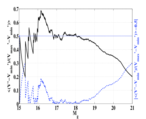
Figure 3: The value of $(V-V_{min})/(V_{max}-V_{min})$ varies along with $m_{max}$ (here denoted as $m_{g}$). In a range from 18 to 21 mag, the trend of the sample forge toward completeness (i.e. $(V-V_{min})/(V_{max}-V{min})=0.5$) as the $m_{max}$ decline is obvious. The sample is of completeness in the range between 17 and 18 mag, and the majority of WDs in the whole sample stand in this range. The large fluctuation between 15 and 17 mag is due to less WDs remaining in this range, which usually leads to large fluctuation in statistics.

We use the method of Schmidt (1968), Green (1980) and Fleming et al. (1986) to calculate the corrections and derive the WD Luminosity Function (LF). Generally, for an all-sky WD sample with upper visual magnitude limit $m_{lim}$, e.g. for $V$ band, given a specific WD with its absolute V magnitude $M_{V}$ and distance $r$, the $r$ defines a volume V, and and the $m_{lim}$ define a maximum distance $r_{max}$ and consequently the maximum volume $V_{max}$ with the following equation: $M_{V}=-5\log r_{max}+m_{lim}+5$ (we assume an average extinction which has been included in $m_{lim}$). The SDSS WD space distribution scale is about 1 $kpc$, whereas the galaxy disk radius is about 10 $kpc$, so it is natural to assume that the WD space radial distribution around the sun is uniform. To correct the non-uniform height distribution, we define $dV(z)=exp(-z/z_{0})dV$ and adopt $z_{0}=250pc$ as the scale height, as done by Fleming et al. (1986) and Liebert et al. (2005). Thus, if the sample is complete, the average value of $V/V_{max}$ will be equal to 0.5 (Green 1980). Otherwise, to make the sample uniform, one should lower the $m_{lim}$ and eliminate the WDs with $V>V_{max}$ until $\langle V/V_{max}\rangle=0.5$.

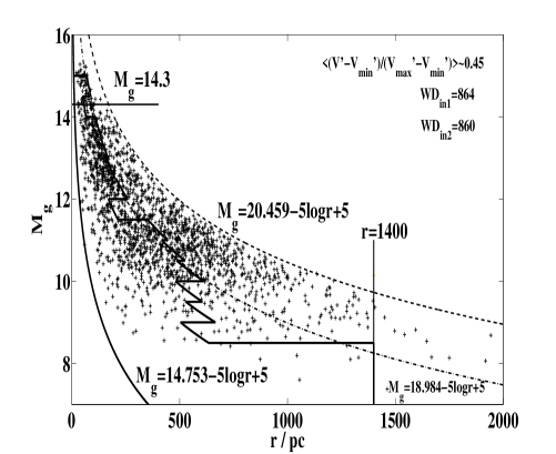
Figure 4: Selection effect correction according to $g$ band and the comparison of the two correction methods. The crosses denote the 1794 SDSS DA WDs with $T_{eff}<48000K$. The left solid line shows the lower $g$ band magnitude limit 14.753 mag and the right dashed line shows the upper magnitude limit 20.459 mag. The middle dot-dashed line is the uniform-correction result with the upper limit 18.984 mag. The sawtooth curve is the bin-correction result giving the upper correction boundary $M_{g}$($r_{max}$). Two straight lines $Mg=14.3$ and $r=14000pc$ also give boundaries out of which the selection effect is relatively severe. There are in total 864 WDs remaining in the sample after the uniform-correction and 860 after the bin-correction.

Moreover, we make two small changes to the method:

(1) In addition to the upper magnitude limit $m_{max}$, the SDSS also has a lower magnitude limit $m_{min}$, which defines a minimum distance $r_{min}$ and a volume $V_{min}$. The reason is that the SDSS’s main focus is extragalactic objects whose magnitudes are usually faint and the WDs are just its spin-off projects (Kleinman et al. 2004). Thus the actual space where WDs were detected is between $r_{min}$ and $r_{max}$, and its volume is $V_{max}-V_{min}$. So we should use $\langle(V-V_{min})/(V_{max}-V_{min})\rangle$ instead of $V_{max}$ to test the sample’s completeness.

(2) The SDSS DR1 spectroscopic data cover only 1360 $deg^{2}$ of the whole sky (Abazajian et al. 2003), so the volume is not a spherical or elliptical shape but a cone shape. We also assume that the $d\Omega(b)$ of the volume $dV$ is apart from its galactic latitude $b$. So the cubic angle $\Omega$ is simply 1360 $deg^{2}$. Then we derive the expression of volume $V$ as a function of $r$ and $b$.

$$V(r,\theta)=\\ \int_{\Omega}{d\Omega\int_{0}^{r}{e^{-z/z_{0}}r^{2}dr}}=\frac{{1360}}{{360^{2}/\pi}}\cdot 4\pi\cdot\leavevmode\nobreak\ \leavevmode\nobreak\ \leavevmode\nobreak\ \leavevmode\nobreak\ \leavevmode\nobreak\ \leavevmode\nobreak\ \leavevmode\nobreak\ \leavevmode\nobreak\ \leavevmode\nobreak\ \leavevmode\nobreak\ \leavevmode\nobreak\ \leavevmode\nobreak\ \leavevmode\nobreak\ \leavevmode\nobreak\ \leavevmode\nobreak\ \leavevmode\nobreak\ \leavevmode\nobreak\ \leavevmode\nobreak\ \leavevmode\nobreak\ \leavevmode\nobreak\ \leavevmode\nobreak\ \leavevmode\nobreak\ \leavevmode\nobreak\ \leavevmode\nobreak\ \\$$

$$\leavevmode\nobreak\ \leavevmode\nobreak\ \leavevmode\nobreak\ (\frac{{z_{0}}}{{\cos\theta}})^{3}\{2-[(\frac{{r\cos\theta}}{{z_{0}}})^{2}+2\frac{{r\cos\theta}}{{z_{0}}}+2]\cdot e^{-r\cos\theta/z_{0}}\},\\$$ (2)

where $\theta=(\pi/2)-b$.

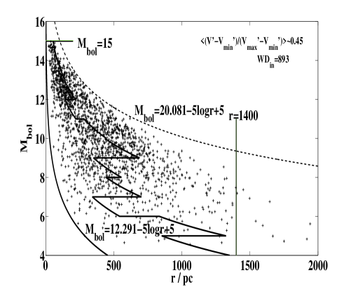
Figure 5: Selection effect bin-correction according to $M_{bol}$. The crosses denote the SDSS 1794 DA WDs with $T_{eff}<48000K$. The left solid line shows the lower bolometric magnitude limit 12.291 mag and the right dashed line shows the upper limit 20.081 mag. The middle sawtooth curve is the bin-correction result giving the upper correction boundary $M_{bol}$($r_{max}$). Two straight lines $M_{bol}=15$ and $r=14000$ pc also give boundaries out of which the selection effect is relatively severe. There are total 893 WDs remaining in the sample after bin-correction.

For $g$ band magnitude, the $(V-V_{min})/(V_{max}-V_{min})$ value of the 1794 non-magnetic SDSS DA WDs with $T_{eff}$ $<$48000K is around 0.3, which suggests that the sample is far from complete. If we lower the the upper magnitude limit $m_{max}$(see Fig. 3) to about 18.2 mag, the $\langle(V-V_{min})/(V_{max}-V_{min})\rangle$ approaches 0.5 and the remaining sample is more complete. However, too many WDs will be eliminated. We made a compromise: if $\mid\langle(V-V_{min})/(V_{max}-V_{min})\rangle-0.5\mid<0.05$, the sample will be regarded as complete. This means that we eliminate the most selection effect contaminated part of the sample. Setting the upper limit $m_{max}=18.984$ for $g$ band, the number of WDs in the remaining sample is 864 out of 1794, almost half (see Fig. 4, we also required $M_{g}<14.3$, for the fainter WDs are difficult to detect). Similarly, Green (1980) also set $V^{\prime}/V_{m}^{\prime}=0.46\pm 0.03$ in his study.

An improved method (hereafter named bin-correction, while the above method is named uniform-correction or ordinary-correction) is to consider the different magnitude upper limit for different absolute magnitudes of a specific WD. We divide the whole sample into 0.5-mag-width bins according to $M_{g}$ (or 1-mag-width bins according to $M_{bol}$), assuming that the WDs within the same bins have the same upper magnitude limit and the whole sample shares a lower magnitude limit. In each bin, $\mid(V-V_{min})/(V_{max}-V_{min})-0.5\mid<0.05$. Fig. 4 shows this bin-correction for $g$ band. The number of WDs in the remaining sample is 860. Although the number is more or less the same as the 864 of the uniform-correction, the difference is obvious: the upper magnitude limit at the brighter end is usually smaller than the 18.984 mag of the uniform-correction. Such WDs observed are relatively distant, whereas the fainter end’s upper magnitude limit is usually larger than the 18.984 mag, because only the faint WDs that are near us can be observed and the magnitude-limiting selection effect is relatively small for the nearby star sample. Thus we prefer to use the improved bin-correction method.

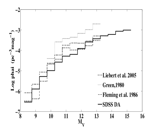
Figure 6: SDSS WD LF as a function of $M_{V}$, compared with previous LFs: dashed, dot-dashed and dotted lines denotes the PG LF of Liebert et al. (2005), LF of Fleming et al. (1986) and LF of Green (1980), respectively. Solid lines denote the SDSS DA WD LF.

We also made a 1-mag-width bin-correction according to $M_{bol}$ for the whole 1794 non-magnetic SDSS DA WD sample with $T_{eff}<48000$K. The number of WDs in the remaining sample is 893, as shown in Fig. 5. The reason why we choose $M_{bol}$ as a criterion is that the u, g, r, i, z or V bands have their own magnitude limits and selection effects. The extinction is also different from short wavelengths to long wavelengths. But above all, the $M_{bol}$ can represent all these factors. After this selection effect correction, our analysis of SDSS WD samples will be much less biased and more reliable.

4 Luminosity function of SDSS DA WDs

The SDSS WD LF is calculated using the method of Green (1980) and Fleming et al. (1986). Its distribution volume is $V_{max}-V_{min}$, and the weight factor is $1/(V_{max}-V_{min})$ which is similar to the $1/V^{\prime}_{m}$ used in some previous studies.

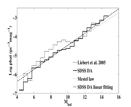
Figure 7: The LF of SDSS WDs as a function of $M_{bol}$, compared with PG LF (Liebert et al. 2005) and theoretical Mestel (1952) law. The dashed line denotes the PG LF by Liebert et al. (2005), while the solid line denotes the SDSS DA WD LF. The dotted-dashed line is the SDSS DA WD LF linear fitting line $\log\Phi=0.3195M_{bol}-7.660$ and the dotted line represents Mestel’s cooling law, $\log\Phi=0.2857M_{bol}-7.330$.

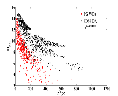
Figure 8: Selection effect comparison. Dots denote PG DA WDs from Liebert et al. (2005) and crosses the SDSS DA WDs after bin-correction. It is clear that in the case of $M_{bol}<8$ mag the PG sample is obviously more dense than the SDSS sample, especially when considering the very large value of $V_{max}-V_{min}$ of SDSS at the brighter magnitude end.

4.1 LF of non-magnetic DA WDs and comparisons with previous results

Fig. 6 shows the LF of SDSS non-magnetic DA WDs (solid line) with $T_{eff}<48000$K and $M_{V}<15.25$. We also show other LFs obtained previously: Liebert et al. (2005, dashed line, called the PG sample and we select WDs with $T_{eff}<48000$K in their sample for comparison); Green (1980, dotted line); Fleming et al. (1986, dot-dashed line). Briefly, the SDSS LF is in general agreement with Liebert et al (2005) and Fleming et al (1986), especially at the fainter end ($M_{V}>12$). An obvious advantage of the SDSS LF is that it extrapolates the fainter end of WD LF from 13.25 to 15.25 mag. Because the SDSS has a lower magnitude limit, WDs with larger $M_{V}$ are usually nearer to us. Their selection effects may not be very strong and the result should be less biased. At the brighter end, however, the SDSS LF is lower by about half an order of magnitude than the PG LF. Some possible reasons that account for such a difference: (1) The PG Survey is an all-sky survey, whereas the SDSS DR1 just covers 1360 $deg^{2}$ of the whole sky. (2) The SDSS sample may contain fewer WDs at the brighter end where $M_{bol}$ $<$7.5. Because SDSS has a low magnitude limit, very bright WDs (with smaller $M_{V}$) must be very distant from us, as shown in Fig. 8. These stars are extremely contaminated by the selection effects and even after the bin-correction the result still may be inaccurate. (3) Fleming et al. (1986) and Liebert et al. (2005) both pointed out that there may be problems of missing binaries or double degenerates in the PG WD sample. Zuckerman & Becklin (1992) and Marsh, Dhillon & Duck (1995) have shown that many low mass DA candidates (usually hot and with low absolute magnitudes) are binaries, with the companion being either a low mass main sequence star or another WD. Kleinman et al. (2004) also mentioned this problem. Bergeron, Leggett & Ruiz (2001) made a detailed analysis of this unresolved problem. Liebert et al. (2005) even pointed out that double degenerates are likely in the majority of cases. So we expect that the missing binaries in the SDSS sample may account for a considerable number of missing stars.

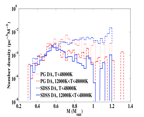
Figure 9: Mass function of SDSS DA WDs in different $T_{eff}$ intervals and the comparison with the PG sample (Liebert et al. 2005). The dot-dashed and dotted lines denote PG DA samples with $12000K<T_{eff}<48000K$ and $T_{eff}<48000K$ from Liebert et al. (2005). The solid and dashed lines denote SDSS DA samples with $12000K<T_{eff}<48000K$ and $T_{eff}<48000K$, respectively. Note that $y$ axis of this figure is a logarithmic scale.

4.2 Comparison with theoretical works

The SDSS DA WD LF is consistent with the theoretical predictions of Mestel (1952) and Lamb & van Horn (1975). The Mestel law is: $Log\phi\propto-(5/7)Log(L/L_{\odot}).$The evolutionary tracks obtained by Lamb & van Horn (1975) also agree with the Mestel law in the $M_{bol}$ range between 6.0 and 13.5. They explained that the deviation below this range is due to the neutrino energy losses and above this range due to the Debye cooling. Compared with these, the SDSS DA WD LF is approximately a straight line in the range of $M_{bol}$ between 6.0 and 13.5, with a linear fitting slope of 0.32, which is almost identical to the slope 2/7 of the Mestel law (Fig. 7). The SDSS DA WD LF also shows a trend of deviation when $M_{bol}$ is smaller than 6.0, which is identical with the model of Lamb & van Horn (1975). For the fainter end where $M_{bol}>13.5$, the LF data does not cover a sufficiently broad $M_{bol}$ range to test the model of Lamb & van Horn (1975).

5 Mass function and space density of SDSS DA WDs

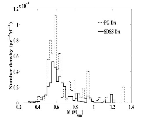
Figure 10: Mass function of SDSS DA WDs (solid line) with $12000K<T_{eff}<48000K$ and the comparison with the 270 DA WDs in PG sample (dashed line) (Liebert et al. 2005).

Fig. 9 shows the mass function (MF), i.e. the $1/(V_{max}-V_{min})$ weighted mass distribution of the SDSS DA WDs. Kleinman et al. (2004) pointed out that the $\log g$ value determination of cooler WDs with $T_{eff}<12000K$ has a systematic offset to higher $\log\ g$ and a possible interpretation is that a moderate amount of helium has been convectively mixed into the atmosphere (see section 6 of Kleinman et al. 2004, also Bergeron et al. 1990; BSL; Liebert et al. 2005). Thus, the parameters and mass functions of WDs with $T_{eff}<12000K$ may be inaccurate. However we include these cool WDs in our MF in Fig. 9 for reference. From both the PG and SDSS MFs in Fig. 9 we can see a qualitative property of MF that in the massive part, the cool WDs’ space density is much larger than that of the hotter WDs. A possible explanation is that the hot massive WDs usually evolve much faster than cool WDs, which leads to its faintness (larger $M_{bol}$) and thus difficulty for observations. So the WDs we observe are usually quite near to us, and consequently have a small $r_{max}$ and larger $1/(V_{max}-V_{min})$ (see Fig. 5 and Fig. 8), which will result in a higher space density. A rough estimate leads to an important implication that cool massive WDs may contribute a larger part to the galactic matter than previous estimates. However, the confirmation of this requires further investigation with more accurate $log\ g$ measurements.

5.1 Non-magnetic DA WD Mass Function

Fig. 10 shows the usually discussed mass function (MF) of WDs with $T_{eff}$ between 12000K and 48000K. It is more accurate because we have more reliable estimates of the masses of these WDs (see discussions in section 2). In many bins, the SDSS DA density is lower than the PG DA density, and the reason is similar to those explained in subsection 4.1. However, their relative distributions are similar. The SDSS MF is also similar to other previous studies, e.g. Wiedemann & Koester (1984), McMahan (1989), BSL, Marsh et al. (1997a), Vennes et al. (1997), Finley et al. (1997) and Napiwotzki et al. (1999), etc. The majority of WDs clump between 0.5 and 0.7 $M_{\odot}$. with some small clusters from 0.7 to 1.0 $M_{\odot}$. Another peak is perhaps seen at 1.2 $M_{\odot}$. Nevertheless, since Kleinman et al. (2004) have artificially assigned an upper $\log g$ limit of 9.0, we obtain no WDs with mass higher than about 1.2 $M_{\odot}$. In other words, the 1.2 $M_{\odot}$ cluster probably includes some WDs more massive than 1.2 $M_{\odot}$. For this reason, Madej et al. (2004) concluded that this peak is not a real feature. Since our sample has been corrected for selection effects and is more complete, we conclude that there really is a cluster and a peak around 1.2 $M_{\odot}$, while the peak may be slightly larger than 1.2 $M_{\odot}$.

5.2 Continuous Mass Function

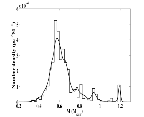
Figure 11: Comparison of the traditional discrete MF and our improved continuous MF of 531 SDSS DA WDs with $12000K<T_{eff}<48000K$

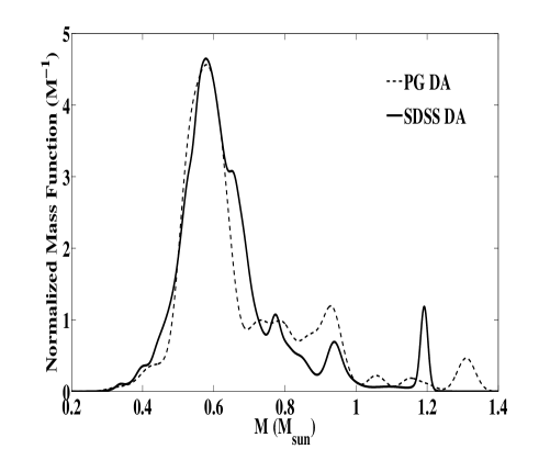
Figure 12: Normalized MF of 531 SDSS DA WDs (solid line) compared to 270 PG DA WDs (Liebert et al. 2005, dashed line), both with $12000K<T_{eff}<48000K$.

Vennes et al. (1997) described a method to derive a continuous MF by calculating $dN_{<M}/dM$, where $N_{<M}$ denotes the number of WDs with mass less than a value M. At each mass point of a WD in the sample, this $dN_{<M}/dM$ will result in a Dirac $\delta$ function. For this reason, they smoothed the function by assuming a Gaussian distribution with a uniform FWHM of 0.1 $M_{\odot}$. Here we try to improve their method. For a specific WD with its observation-derived mass $M_{i}$ and error $\sigma M_{i}$, the probability density function of this WD is a Gaussian distribution function. The probability that this WD’s mass equals M is equal to $\Psi_{i}(M)dM=\frac{1}{{\sqrt{2\pi}\sigma_{Mi}}}\exp\{-\frac{{(M-M_{i})^{2}}}{{2\sigma_{Mi}^{2}}}\}dM$ and $\int{\Psi_{i}(M)dM}=1$. So the mass function here can be defined as:

$$\rho(M)=\sum\limits_{i}{\frac{1}{{V_{\max i}-V_{\min i}}}\Psi_{i}(M)}\leavevmode\nobreak\ \leavevmode\nobreak\ \leavevmode\nobreak\ \leavevmode\nobreak\ \leavevmode\nobreak\ \leavevmode\nobreak\ \leavevmode\nobreak\ \leavevmode\nobreak\ \leavevmode\nobreak\ \leavevmode\nobreak\ \leavevmode\nobreak\ \leavevmode\nobreak\ \leavevmode\nobreak\ \leavevmode\nobreak\ \leavevmode\nobreak\ \leavevmode\nobreak\ \leavevmode\nobreak\ \leavevmode\nobreak\ \leavevmode\nobreak\ \leavevmode\nobreak\ \leavevmode\nobreak\ \leavevmode\nobreak\ \leavevmode\nobreak\ \leavevmode\nobreak\ \leavevmode\nobreak\ \leavevmode\nobreak\ \leavevmode\nobreak\$$

$$\leavevmode\nobreak\ \leavevmode\nobreak\ \leavevmode\nobreak\ =\sum\limits_{i}{\frac{1}{{V_{\max i}-V_{\min i}}}\frac{1}{{\sqrt{2\pi}\sigma_{Mi}}}\exp\{-\frac{{(M-M_{i})^{2}}}{{2\sigma_{Mi}^{2}}}\}}.$$ (3)

This is the detected or observed space density. The total space density is $\rho_{tot}=\sum\limits_{i}{\frac{1}{{V_{\max i}-V_{\min i}}}}$ and the normalized mass function will be: $\rho_{norm}(M)=\rho(M)/\rho_{tot}$

Usually, the error of a SDSS WD mass is small enough to retain its distribution properties and also large enough not to produce a Dirac $\delta$ function. Fig. 11 compares the traditional discrete MF and our continuous MF of SDSS DA WDs with $T_{eff}$ between 12000K and 48000K. They are in good agreement and thus demonstrate the reliability of our method. The continuous MF has many advantages over the discrete one. From it, we determine that the main peak of the SDSS DA mass distribution is at M=0.58 $M_{\odot}$ and two other obvious peaks at M=0.94 $M_{\odot}$ and M=1.19$M_{\odot}$. The 0.58$M_{\odot}$ peak is in perfect agreement with previous studies (see Table 1 of Madej et al. 2004). The 0.58$M_{\odot}$ peak, which is derived from $1/(V_{max}-V_{min})$ weighted MF of a complete sample after selection effect corrections, is close to the 0.562$M_{\odot}$ peak derived by Madej et al. (2004), found by simply counting the number of WDs in an incomplete sample. This implies that the main peak of the WD mass distribution around 0.57 $M_{\odot}$ is very insensitive to sample completeness, which puts in context the agreement of our results with previous studies.

5.3 Total space density and normalized mass function

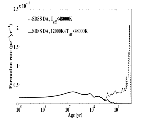
Figure 13: Detailed formation rates of SDSS WDs in linear and log Age scale. The dashed lines denote SDSS DA samples with $T_{eff}<48000K$. The solid lines denote SDSS DA samples with $12000K<T_{eff}<48000K$ .

The total space density of SDSS DA WDs is $8.81\times 10^{-5}pc^{-3}$ for WDs with $T_{eff}$ between 12000K and 48000K and $1.94\times 10^{-3}pc^{-3}$ for WDs with $T_{eff}<48000K$. If we include DB/DO WDs, the result will be $1.10\times 10^{-4}pc^{-3}$ and $2.51\times 10^{-3}$ pc-3, respectively. The normalized MF is shown in Fig. 12, assuming that the average error for the PG DA WD masses is 0.025 $M_{\odot}$, equal to the bin-width of the discrete MF to retain the distribution information. The two normalized MFs agree well and show similar properties of distribution when $M<1.0M_{\odot}$, e.g. the main peak around 0.57 $M_{\odot}$ and its width (FWHM), despite the SDSS DR1 just covering a small area of the whole sky. As we discussed in section 6.2, if the artificial $\log g=9.0$ limit is relaxed, the SDSS 1.2 $M_{\odot}$ high and thin peak would be lower and wider and move right-ward, more like the PG 1.3 $M_{\odot}$ peak. Our conclusion is that there is a small peak around or above 1.2 $M_{\odot}$.

6 The formation rate of SDSS WDs

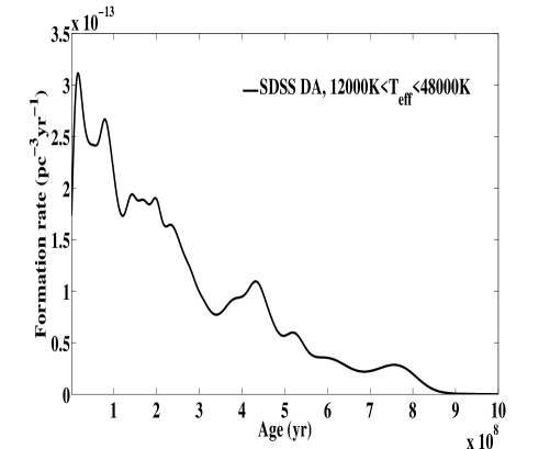
Figure 14: Detailed formation rates of SDSS WDs with $12000K<T_{eff}<48000K$.

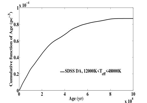
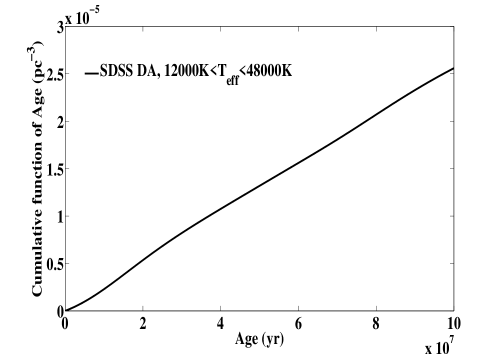
Figure 15: Cumulative Age Functions of SDSS WDs with $12000K<T_{eff}<48000K$ in the last 1 Gyrs (upper panel) and 0.1 Gyrs (lower panel). It clearly shows a declining slope with age, which implies a decline of the formation rate. Yet in the last 0.1 Gyrs, the curve is nearly a straight line.

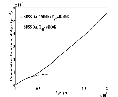
Figure 16: Cumulative Age Functions of SDSS WDs with $T_{eff}<48000K$. The dashed lines denote SDSS DA samples with $T_{eff}<48000K$. The solid lines denote SDSS DA samples with $12000K<T_{eff}<48000K$. Dashed curves in the upper figure show variable slope as age goes old, which implies the variation of the formation rate. Yet in the last 2 Gyrs, the curves are nearly two straight lines.

When we substitute WD age for the mass $M$ in the continuous MF, we will obtain the age Function, as shown in Fig. 13. In fact, this age function is just the WD formation rate as a function of Age (see Fig. 14). Although the subtle details will be contaminated by fluctuation, the general trend is much more reliable. Considering the complete sample with $T_{eff}<48000K$, including 893 WDs, we find a relatively constant formation rate of about $0.3\sim 0.4\times 10^{-12}pc^{-3}yr^{-1}$ during the last 2 Gyrs. There is a very high formation rate peak around $3\sim 3.5$ Gyr (see dashed line in Fig. 13). The real peak may not be as high as is shown because of the artificial upper limit of $\log g=9.0$ by Kleinman et al. (2004). The massive WDs, according to current SDSS data and models, are usually very old. If we consider only the 531 WDs with $12000K<T_{eff}<48000K$, another problem is seen: the formation rate declines rapidly when the WD’s age exceeds 0.1 Gyr (see Fig. 14). Liebert et al. (2005) noticed this fact as well (see section 5.1 and Fig. 16 of their paper). An interpretation can be found: when we just consider the hotter WDs, the sample will be incomplete due to the elimination of the cooler ones which were much hotter many years ago when they were born. So the formation rate of the hotter sample will decline rapidly accompanying the WDs’ cooling along time. The same thing happens in the EUVE Survey sample (see Fig. 9 in Vennes et al. (1997)). In their sample the formation rate declines even faster (at 10 Myr) than in our work and Liebert et al. (2005) because their sample is hotter than 20000K. The hotter the sample is, the more incomplete it is and the more rapidly the formation rate declines. We integrate the Age (birth rate) Function to get the Cumulative Age Function as shown in Fig. 15 and Fig. 16, which are similar to Fig. 9 in Vennes et al. (1997). In Fig. 15, the hotter sample shows a nearly excellent straight line below 0.1 Gyr. By assuming a constant formation rate in the last 2 Gyrs to eliminate the influence of the fluctuation in the continuous function, we can make a linear fit to obtain an average formation rate equal to the fitting line’s slope. The complete sample also exhibits a straight line below 2 Gyr, as is shown in Fig. 16. The result is $2.579\times 10^{-13}pc^{-3}yr^{-1}$ and $2.794\times 10^{-13}pc^{-3}yr^{-1}$, for WDs with $12000K<T_{eff}<48000K$ and $T_{eff}<48000K$, respectively. If the formation rate is corrected for nondegenerate companions and for those WDs that are likely to be in binaries, it will be increased by a significant factor. Compared with the recent calculated PNe formation rate of about $(2.1\sim 3)\times 10^{-12}pc^{-3}yr^{-1}$ (Pottasch 1996; Phillips 2002), there is a significant disagreement (see the detailed discussion in section 5.7 of Liebert et al. 2005). Previous calculated WD formation rates have also been listed in Table 3 for comparison with our result.

7 Three-dimension distribution function and the H-R diagram

Bergeron et al. (2001) have emphasized the importance of combining the MF and LS into one distribution function for the comparison of cooling time. The LF and other parameters of a sample of WDs vary in different mass groups. For this reason, Liebert et al. (2005) divided the whole PG sample into 3 groups with mass around 0.6 $M_{\odot}$, $M<0.46M_{\odot}$ and $M>0.8M_{\odot}$, respectively. Their discussions of the other parameters such as the formation rate are all based on this 3-group division. However, this method also has some problems. (1) Even within each group, the distribution and parameters are not uniform. (2) This 3-group division method is not universal, e.g. in the SDSS sample, as is shown in Fig. 10 and Fig. 12, this division is not appropriate because the 0.578 $M_{\odot}$ peak is too strong, overwhelming the other groups and the 1.19 $M_{\odot}$ peak is unreliable. Using the continuous distribution function we proposed above, a more universal solution can be found by assuming that every WD’s contribution to the space density can be described as a 2-Dimensional Gaussian distribution weighted by $1/(V_{max}-V_{min})$. We define the Mass-Luminosity Function (MLF) as:

$$\rho(M,M_{bol})=\\ \sum\limits_{i}{(\frac{1}{{V_{\max,i}-V_{\min,i}}}\cdot\frac{1}{{2\pi\sigma_{M_{i}}\cdot\sigma_{M_{bol,i}}}}\cdot}$$

$$\leavevmode\nobreak\ \leavevmode\nobreak\ \leavevmode\nobreak\ \leavevmode\nobreak\ \leavevmode\nobreak\ \leavevmode\nobreak\ \leavevmode\nobreak\ \leavevmode\nobreak\ \leavevmode\nobreak\ \leavevmode\nobreak\ \leavevmode\nobreak\ \leavevmode\nobreak\ \leavevmode\nobreak\ \leavevmode\nobreak\ \leavevmode\nobreak\ \exp\{-\frac{{(M-M_{i})^{2}}}{{2\sigma_{M,i}^{2}}}-\frac{{(M-M_{bol,i})^{2}}}{{2\sigma_{M_{bol,i}}^{2}}}\})\\$$ (4)

One can substitute the age, $T_{eff}$ or other parameters for $M$ or $M_{bol}$ in Eq. (4) to obtain other 3-D distribution functions.

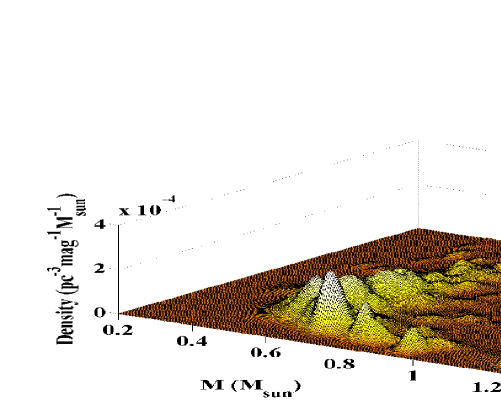
Figure 17: 3-Dimension Mass-Luminosity Function for SDSS DA WDs with $12000K<T_{eff}<48000K$.

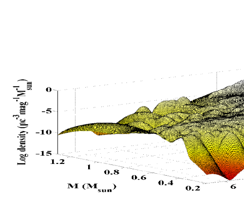
Figure 18: 3-Dimension Mass-Luminosity Function for SDSS DA WDs with $T_{eff}<48000K$. Note that the z axis is in log scale. The red part which has the highest value shows the trend that the mass peak moves toward the high mass end as $M_{bol}$ becomes higher.

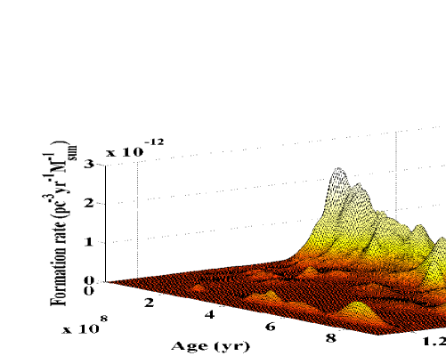
Figure 19: Mass-age distribution function for SDSS DA WDs with $12000K<T_{eff}<48000K$ (upper) and $T_{eff}<48000K$ (lower). The mass peak has a explicit trace toward the high mass end when the age increases.

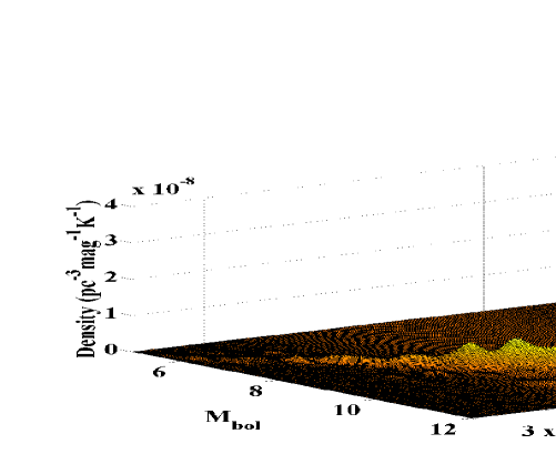
Figure 20: H-R diagram for SDSS DA WDs with $12000K<T_{eff}<48000K$. $T_{eff}$ axis is in $\log$ scale and the left end has a larger value.

Fig. 17 shows the mass-luminosity function for SDSS DA WDs with $12000K<T_{eff}<48000K$. The main cluster in Fig. 12 with many subtle peaks is now decomposed into a ’mountain’ along $M_{bol}$ with several independent peaks. In this figure, the maximum mass distribution peak is at about 0.65 $M_{\odot}$, which is just a quasi-peak in Fig. 12, and the overwhelming peak at 0.58 $M_{\odot}$ is the integration along $M_{bol}$ of the ’mountain ridge’ at about 0.55 $M_{\odot}$. We can also see a trend that the mass cluster moves to the massive end as the $M_{bol}$ goes to the fainter end. Thus, we can infer that if the $M_{bol}$ becomes fainter than 12 mag, the mass cluster will continue to move to the massive end, and in Fig. 18 we confirm this inference. This trend is partly interpreted by Fig. 19. If we assume that most of the progenitors of these WDs formed almost simultaneously at early stage of our galaxy, as massive stars usually evolve faster than lighter ones, they will soon die out to produce massive WDs and have a long cooling time to reach a present high $M_{bol}$. Meanwhile the less massive stars have much longer lives and die slowly and much later to give birth to recently born WDs, which have had little time to cool and only retain a low $M_{bol}$. This implies that the mass - age distribution of a complete WD sample contains important information on the early main sequence stars and our galaxy. Fig. 20 gives the 3-D H-R diagram which shows an obvious evolutionary track of WDs.

8 Discussion and summary

We have performed a study of a DA WD sample from SDSS DR1. To ensure that our adopted sample is accurate and complete, we have carried out many tests. We performed a mass determination comparison to test the accuracy of the model of Panei et al. (2000). By comparing the model-derived mass with that obtained from other methods, independent of the theoretical M-R relation, we find that the model of Panei et al. (2000) is reliable enough to be applied to the mass estimation of SDSS WDs, especially for the hotter WDs.

We tested the completeness of the SDSS WD sample and corrected for selection effects. We found that this sample is far from complete, mainly due to the magnitude-limiting selection effect. Thus we lower the upper magnitude limit by at least 1.5 mag to make the sample almost complete. We also proposed a more detailed bin-correction method to improve the accuracy. The remaining 531 DA WDs with $12000K<T_{eff}<48000K$ still form the largest homogeneous and complete DA WD sample to date.

We calculated the SDSS WD Luminosity Function based on the methods of Green (1980) and Fleming et al. (1986), except for some minor differences. The SDSS LF is generally in agreement with most previous studies. In addition, the SDSS LF itself shows excellent agreement with theoretical work, e.g. the Mestel law. We also proposed some possible interpretations to account for the disagreements between the SDSS and PG WD samples. We then introduced an improved continuous mass function and a method to obtain the 2-dimensional distribution functions. We derived a SDSS MF whose relative distribution and properties are in good agreement with that of the PG sample, although the absolute value is different. We thus obtained a 0.58 $M_{\odot}$ mass peak and found that in the 2-D Mass-Luminosity Function it is decomposed into a ’mountain ridge’ along $M_{bol}$ at about 0.55 $M_{\odot}$ and an actual peak at about 0.65 $M_{\odot}$ for fainter WDs. Evidence implies that there is a massive WD peak or cluster above 1.2 $M_{\odot}$, which mainly consists of cool and faint WDs. The derived space density is $8.81\times 10^{-5}pc^{-3}$ and the formation rate is about $2.579\times 10^{-13}pc^{-3}yr^{-1}$ and $2.794\times 10^{-13}pc^{-3}yr^{-1}$, for SDSS DA WDs with $12000K<T_{eff}<48000K$ and $T_{eff}<48000K$, respectively.

As predicted by Kleinman et al. (2004), we can expect an additional 10,000 WDs or so by the time the SDSS is finished; a much larger and more complete sample of WDs will be available. Eisentein et al. (2006) published a catalog of 9316 spectroscopically confirmed WDs from the SDSS DR4, which includes 8000 DA WDs. A further study of the statistical properties of WDs with this enlarged sample is under way and will be reported in a future work. The theortical model of WDs adopted in our study is still quite simple. Any future progress in the theoretical models of WDs would be very helpful for a more accurate understanding of the statistical properties of WDs.

Table 1: Comparison of white dwarf mass determinations from different methods

Name	$T_{eff}$	$log\ g$	$M_{spec}$	$M_{other}$	Notes	Ref.
	(K)		($M_{\sun}$)	($M_{\sun}$)
Sirius B	24700 $\pm$ 300	8.61 $\pm$ 0.04	0.998 $\pm$ 0.024	1.003 $\pm$ 0.016	1	1,3
40 Eri B	16700 $\pm$ 300	7.77 $\pm$ 0.01	0.493 $\pm$ 0.006	0.501 $\pm$ 0.011	1	1,4
Sirius B	25193 $\pm$ 37	8.566 $\pm$ 0.01	0.978 $\pm$ 0.005	1.02 $\pm$ 0.02	2	14
GD279	13500 $\pm$ 200	7.83 $\pm$ 0.03	0.514 $\pm$ 0.016	0.44 $\pm$ 0.02	2	1,12
Feige 22	19100 $\pm$ 400	7.78 $\pm$ 0.04	0.505 $\pm$ 0.020	0.41 $\pm$ 0.03	2	1,12
EG21	16200 $\pm$ 300	8.06 $\pm$ 0.05	0.649 $\pm$ 0.030	0.5 $\pm$ 0.02	2	1,12
EG50	21000 $\pm$ 300	8.10 $\pm$ 0.05	0.682 $\pm$ 0.030	0.58 $\pm$ 0.05	2	1,12
GD140	21700 $\pm$ 300	8.48 $\pm$ 0.05	0.917 $\pm$ 0.031	0.79 $\pm$ 0.02	2	1,12
G226-29	12000 $\pm$ 200	8.29 $\pm$ 0.03	0.784 $\pm$ 0.019	0.75 $\pm$ 0.03	2	1,12
WD2007-303	15200 $\pm$ 700	7.86 $\pm$ 0.05	0.534 $\pm$ 0.028	0.44 $\pm$ 0.05	2	1,12
Wolf1346	20000 $\pm$ 300	7.83 $\pm$ 0.05	0.532 $\pm$ 0.026	0.44 $\pm$ 0.01	2	1,12
G93-48	18300 $\pm$ 300	8.02 $\pm$ 0.05	0.630 $\pm$ 0.029	0.75 $\pm$ 0.06	2	1,12
L711-10	19900 $\pm$ 400	7.93 $\pm$ 0.05	0.584 $\pm$ 0.028	0.54 $\pm$ 0.04	2	1,12
CD-38 10980	24000 $\pm$ 200	7.92 $\pm$ 0.04	0.588 $\pm$ 0.021	0.74 $\pm$ 0.04	2	1,12
Wolf 485A	14100 $\pm$ 400	7.93 $\pm$ 0.05	0.570 $\pm$ 0.018	0.59 $\pm$ 0.04	2	1,12
G154-B5B	14000 $\pm$ 400	7.71 $\pm$ 0.05	0.457 $\pm$ 0.015	0.53 $\pm$ 0.05	2	1,12
G181-B5B	13600 $\pm$ 500	7.79 $\pm$ 0.05	0.495 $\pm$ 0.016	0.46 $\pm$ 0.08	2	1,12
G238-44	20200 $\pm$ 400	7.90 $\pm$ 0.05	0.568 $\pm$ 0.028	0.42 $\pm$ 0.01	2	1,12
LB 1497	31660 $\pm$ 350	8.78 $\pm$ 0.049	1.097 $\pm$ 0.025	1.025 $\pm$ 0.043	3,5	2,6,12
HZ 4	14770 $\pm$ 350	8.16 $\pm$ 0.049	0.707 $\pm$ 0.032	0.632 $\pm$ 0.042	3,5	2,7,12
GH 7-112	15190 $\pm$ 350	8.3 $\pm$ 0.049	0.795 $\pm$ 0.031	0.783 $\pm$ 0.039	3,5	2,7,12
40 Eri B	16570 $\pm$ 350	7.86 $\pm$ 0.049	0.538 $\pm$ 0.026	0.52 $\pm$ 0.4	3,5	2,8,12
GH 7-191	19570 $\pm$ 350	8.09 $\pm$ 0.049	0.674 $\pm$ 0.030	0.669 $\pm$ 0.036	3,5	2,7,12
GH 7-233	24420 $\pm$ 350	8.11 $\pm$ 0.049	0.695 $\pm$ 0.029	0.617 $\pm$ 0.028	3,5	2,7,12
HZ 7	21340 $\pm$ 350	8.04 $\pm$ 0.049	0.648 $\pm$ 0.029	0.665 $\pm$ 0.077	3,5	2,7,12
HZ 14	27390 $\pm$ 350	8.07 $\pm$ 0.049	0.678 $\pm$ 0.028	0.51 $\pm$ 0.086	3,5	2,7,12
G191-B2B	64100 $\pm$ 350	7.69 $\pm$ 0.049	0.580 $\pm$ 0.010	0.538 $\pm$ 0.043	3,5	2,10,12
G163-50	15070 $\pm$ 350	7.83 $\pm$ 0.049	0.519 $\pm$ 0.026	0.465 $\pm$ 0.046	3,5	2,5,12
G148-7	15480 $\pm$ 350	7.97 $\pm$ 0.049	0.595 $\pm$ 0.028	0.558 $\pm$ 0.038	3,5	2,8,12
Wolf 485A	14100 $\pm$ 350	7.93 $\pm$ 0.049	0.570 $\pm$ 0.028	0.529 $\pm$ 0.042	3,5	2,5,12
L762-21	18580 $\pm$ 350	8.32 $\pm$ 0.049	0.813 $\pm$ 0.032	0.808 $\pm$ 0.099	3,5	2,5,12
G154-B5B	13950 $\pm$ 350	7.71 $\pm$ 0.049	0.457 $\pm$ 0.024	0.524 $\pm$ 0.04	3,5	2,8,12
G142-B2A	14040 $\pm$ 350	7.84 $\pm$ 0.049	0.521 $\pm$ 0.026	0.561 $\pm$ 0.037	3,5	2,8,12
L587-77A	9330 $\pm$ 350	7.87 $\pm$ 0.049	0.524 $\pm$ 0.028	0.657 $\pm$ 0.035	3,4,5	2,5,12
G86-B1B	9140 $\pm$ 350	8.3 $\pm$ 0.049	0.785 $\pm$ 0.032	0.454 $\pm$ 0.118	3,4,5	2,11,12
G111-71	7710 $\pm$ 350	8.15 $\pm$ 0.049	0.685 $\pm$ 0.032	0.632 $\pm$ 0.125	3,4,5	2,11,12
G116-16	8750 $\pm$ 350	8.29 $\pm$ 0.049	0.778 $\pm$ 0.032	1.009 $\pm$ 0.06	3,4,5	2,11,12
G121-22	10260 $\pm$ 350	6.12 $\pm$ 0.049	0.651 $\pm$ 0.035	1.084 $\pm$ 0.023	3,4,5	2,11,12
G61-17	11000 $\pm$ 350	8.04 $\pm$ 0.049	0.626 $\pm$ 0.030	0.552 $\pm$ 0.038	3,4,5	2,11,12
L619-50	10080 $\pm$ 350	8.17 $\pm$ 0.049	0.703 $\pm$ 0.032	0.502 $\pm$ 0.069	3,4,5	2,5,12
LP696-4	10470 $\pm$ 350	8.11 $\pm$ 0.049	0.667 $\pm$ 0.031	0.44 $\pm$ 0.12	3,4,5	2,11,12
LP25-436	8440 $\pm$ 350	8.52 $\pm$ 0.049	0.926 $\pm$ 0.032	0.644 $\pm$ 0.056	3,4,5	2,11,12
G156-64	7160 $\pm$ 350	8.43 $\pm$ 0.049	0.866 $\pm$ 0.032	0.548 $\pm$ 0.052	3,4,5	2,11,12
G216-B24B	9860 $\pm$ 350	8.2 $\pm$ 0.049	0.722 $\pm$ 0.032	0.832 $\pm$ 0.047	3,4,5	2,11,12
L557-71	8780 $\pm$ 350	8.29 $\pm$ 0.049	0.778 $\pm$ 0.032	0.549 $\pm$ 0.038	3,4,5	2,11,12
G19-20	13620 $\pm$ 350	7.79 $\pm$ 0.049	0.495 $\pm$ 0.025	0.489 $\pm$ 0.084	3,5	2,5,12

Note: $M_{spec}$ refers to spectroscopic mass derived with the evolutionary model of Panei(2000) from the spectral parameters($T_{eff}$ and $log\ g$) and $M_{other}$ refers to the mass derived from 1: orbital parameters, 2: parallaxes and $log\ g$, and 3: gravitational redshift. Note 4 denotes low temperature WDs ($T_{eff}$ $<$12000K) and 5 denotes that the individual errors of $T_{eff}$ and $log\ g$ of each WD is not available, so we assumed the errors of $T_{eff}$ and $log\ g$ being the mean errors of the sample the WD belongs to.

References: (1) Provencal et al. (1998); (2) Bergeron et al. (1995a); (3) Gatewood & Gatewood (1978); (4) Shipman et al. (1997); (5) Koester (1987) (6) Wegner, Reid & McMahan (1991) (7) Wegner, Reid & McMahan (1989); (8) Wegner & Reid (1987); (9) Koester & Weidemann (1991); (10) Reid & Wegner (1988); (11) Wegner & Reid (1991); (12) BSL and Bragaglia et al. (1995); (13) McCook & Sion (1999); (14) Barstow et al. (2005).

Table 2: Fundamental parameters of the DA white dwarfs from the Sloan Digital Sky Survey

Object name	SDSS No.	$T_{eff}$	$log\ g$	Mass	Radius	Age	$M_{bol}$	$M_{g}$	Distance
		(K)		($M_{\sun}$)	($\frac{R_{\sun}}{100}$)	(yr)			(pc)
002509 - 104048	1189	16390 $\pm$ 480	7.74 $\pm$ 0.12	0.48 $\pm$ 0.06	1.54 $\pm$ 0.12	9.48E+07	9.27	10.63	555 $\pm$ 26
020747 + 121028	1210	16661 $\pm$ 2104	8.37 $\pm$ 0.23	0.84 $\pm$ 0.14	0.99 $\pm$ 0.18	3.19E+08	10.16	11.57	371 $\pm$ 55
023907 + 002917	1198	16449 $\pm$ 467	7.86 $\pm$ 0.11	0.54 $\pm$ 0.06	1.43 $\pm$ 0.11	1.14E+08	9.43	10.80	554 $\pm$ 24
024855 - 004139	1175	16180 $\pm$ 390	7.87 $\pm$ 0.08	0.54 $\pm$ 0.04	1.42 $\pm$ 0.08	1.24E+08	9.52	10.84	417 $\pm$ 14
025746 + 010106	1208	16628 $\pm$ 214	8.30 $\pm$ 0.04	0.80 $\pm$ 0.03	1.05 $\pm$ 0.03	2.78E+08	10.06	11.46	149 $\pm$ 3
030028 - 084126	1185	16364 $\pm$ 505	7.90 $\pm$ 0.11	0.56 $\pm$ 0.06	1.39 $\pm$ 0.10	1.25E+08	9.51	10.87	514 $\pm$ 23
031232 - 060907	1172	16164 $\pm$ 373	7.86 $\pm$ 0.08	0.54 $\pm$ 0.04	1.43 $\pm$ 0.08	1.22E+08	9.51	10.83	438 $\pm$ 15
032126 - 061442	1187	16374 $\pm$ 340	7.83 $\pm$ 0.07	0.52 $\pm$ 0.04	1.46 $\pm$ 0.07	1.11E+08	9.41	10.76	458 $\pm$ 14
032947 + 010050	1204	16590 $\pm$ 726	8.59 $\pm$ 0.12	0.98 $\pm$ 0.07	0.83 $\pm$ 0.08	4.52E+08	10.57	11.97	324 $\pm$ 20
032960 - 000733	1193	16406 $\pm$ 326	7.76 $\pm$ 0.07	0.49 $\pm$ 0.03	1.52 $\pm$ 0.07	9.83E+07	9.30	10.66	417 $\pm$ 12

Note: A subset of the table is shown here. The complete table is available electronically upon request.

Table 3: Comparisons of our calculated WD formation rate with previous results

Formation rate $(pc^{-3}yr^{-1})$	Sample	Reference
$2.58\times 10^{-13}$	531 DA WDs from SDSS	this work
$(0.1-2)\times 10^{-10}$	89 WDs	Green (1980)
$(3.9-6.1)\times 10^{-13}$	353 DA WDs from PG	Fleming et al. (1986)
$2.3\times 10^{-12}$		Weidemann (1991)
$(7-10)\times 10^{-13}$	90 hot WDs from EUVE	Vennes et al. (1997)
$6\times 10^{-13}$	348 DA WDs from PG	Liebert et al. (2005)