The XMM–Newton wide-field survey in the COSMOS field II: X-ray data and the logN-logS

Abstract

We present the data analysis and the X–ray source counts for the first season of XMM–Newton  observations in the COSMOS field. The survey covers $\sim$2 deg² within the region of sky bounded by $9^{h}57.5^{m}<R.A.<10^{h}03.5^{m}$; $1^{d}27.5^{m}<DEC<2^{d}57.5^{m}$ with a total net integration time of 504 ks. A maximum likelihood source detection was performed in the 0.5–2 keV, 2–4.5 keV and 4.5–10 keV energy bands and 1390 point-like sources were detected in at least one band. Detailed Monte Carlo simulations were performed to fully test the source detection method and to derive the sky coverage to be used in the computation of the logN-logS relations. These relations have been then derived in the 0.5–2 keV, 2–10 keV and 5–10 keV energy bands, down to flux limits of 7.2$\times$10^-16 erg cm^-2 s^-1, 4.0$\times$10^-15 erg cm^-2 s^-1 and 9.7$\times$10^-15 erg cm^-2 s^-1, respectively. Thanks to the large number of sources detected in the COSMOS survey, the logN-logS curves are tightly constrained over a range of fluxes which were poorly covered by previous surveys, especially in the 2–10 and 5–10 keV bands. The 0.5–2 keV and 2–10 keV differential logN-logS were fitted with a broken power-law model which revealed a Euclidean slope ($\alpha\sim$2.5) at the bright end and a flatter slope ($\alpha\sim$1.5) at faint fluxes. In the 5–10 keV energy band a single power-law provides an acceptable fit to the observed source counts with a slope $\alpha\sim$2.4. A comparison with the results of previous surveys shows good agreement in all the energy bands under investigation in the overlapping flux range. We also notice a remarkable agreement between our logN-logS relations and the most recent model of the XRB. The slightly different normalizations observed in the source counts of COSMOS and previous surveys can be largely explained as a combination of low counting statistics and cosmic variance introduced by the large scale structure.

1. Introduction

The source content of the X–ray sky has been investigated over a broad range of fluxes and solid angles thanks to a large number of deep and wide surveys performed in the last few years using ROSAT, Chandra and XMM–Newton  (see Brandt & Hasinger 2005 for a review). Follow–up observations unambiguously indicate that Active Galactic Nuclei (AGN), many of which are obscured, dominate the global energy output recorded in the cosmic X–ray background. The impressive amount of X–ray and multi-wavelength data obtained to date have opened up the quantitative study of the demography and evolution of accretion driven Supermassive Black Holes (SMBHs; Miyaji et al., 2000; Hasinger et al., 2005; Ueda et al., 2003; La Franca et al., 2005). At present the two deepest X–ray surveys, the Chandra Deep Field North (CDFN; Bauer et al., 2004) and Chandra Deep Field South (CDFS; Giacconi et al., 2001), have extended the sensitivity by about two orders of magnitude in all bands with respect to previous surveys (Hasinger et al., 1993; Ueda et al., 1999; Giommi et al., 2000), detecting a large number of faint X–ray sources. However, deep pencil beam surveys are limited by the area which can be covered to very faint fluxes (typically of the order of 0.1 deg²) and suffer from significant field to field variance. In order to cope with such limitations, shallower surveys over larger areas have been undertaken in the last few years with both Chandra (e.g. the 9 deg² Bootes survey (Murray et al., 2005), the Extended Groth strip EGS (Nandra et al., 2005), the Extended Chandra Deep Field South E-CDFS, (Lehmer et al., 2005; Virani et al., 2006) and the Champ (Green et al., 2004; Kim et al., 2004)) and XMM–Newton (e.g. the HELLAS2XMM survey (Fiore et al., 2003), the XMM–Newton  BSS (Della Ceca et al., 2004) and the ELAIS S1 survey (Puccetti et al., 2006) ).

In this context the XMM–Newton  wide field survey in the COSMOS field (Scoville et al., 2007), hereinafter XMM–COSMOS (Hasinger et al., 2007), has been conceived and designed to maximize the sensitivity and survey area product, and is expected to provide a major step forward toward a complete characterization of the physical properties of X–ray emitting SMBHs. A contiguous area of about 2 deg² will be covered by 25 individual pointings, repeated twice, for a total exposure time of about 60 ksec in each field. In the first observing run obtained in AO3 (phase A), the pointings were disposed on a 5x5 grid with the aimpoints shifted of 15’ each other, so as to produce a contiguous pattern of coverage. In the second run, to be observed in AO4 (phase B), the same pattern will be repeated with each pointing shifted by 1’ with respect to phase A. The above described approach ensures a uniform and relatively deep coverage of more than 1 deg² in the central part of the field. When completed, XMM–COSMOS will provide an unprecedentedly large sample of about 2000 X–ray sources with full multi-wavelength photometric coverage and a high level of spectroscopic completeness. As a consequence, the XMM–COSMOS survey is particularly well suited to address AGN evolution in the context of the Large Scale Structure in which they reside. More specifically, it will be possible to investigate if obscured AGN are biased tracers of the cosmic web and whether their space density rises in the proximity of galaxy clusters (Henry & Briel, 1991; Cappi et al., 2001; Gilli et al., 2003; Johnson et al., 2003; Yang et al., 2003; Cappelluti et al., 2005; Ruderman & Ebeling, 2005; Miyaji et al., 2007; Yang et al., 2006; Cappelluti et al., 2006).
The X–ray reduction of phase A data along with a detailed analysis of the source counts in different energy bands are presented in this paper which is organized as follows. In Section 2 the data reduction procedure and the relative astrometric corrections are described. In Section 3 the source detection algorithms and technique are discussed. Monte Carlo simulations are presented in Section 4. The logN–logS relations and the analysis of the contribution of the XMM-COSMOS sources to the X-ray background are discussed in Section 5. The study of sample variance is presented in Section 6 and a summary of the work is reported in Section 7. The strategy and the log of the observations of XMM–COSMOS are presented by Hasinger et al. (2007), the optical identifications of X-ray sources by Brusa et al. (2007), the analysis of groups and clusters by Finoguenov et al. (2007), the spectral analysis of a subsample of bright sources by Mainieri et al. (2007) and the clustering of X-ray extragalactic sources by Miyaji et al. (2007). Throughout the paper the concordance WMAP $\Lambda$CDM cosmology (Spergel et al., 2003) is adopted with H₀=70 km s^-1 Mpc^-1, $\Omega_{\Lambda}$=0.7 and $\Omega_{m}$=0.3

2. EPIC Data cleaning

The EPIC data were processed using the XMM–Newton  Standard Analysis System (hereinafter SAS) version 6.5.0. The Observational Data Files (ODF, ”raw data”) of each of the 25 observations, were calibrated using the SAS tools epchain and emchain with the most recent calibration data files. Events in bad columns, bad pixels and close to the chip gaps were excluded.
Both the EPIC PN and MOS event files were searched for high particle background intervals. The distribution of the background counts binned in 100 s intervals was obtained in the 12–14 keV band for the PN and in the 10–12 keV band for the MOS, which are dominated by particle background, and then fitted with a gaussian model. All time intervals with background count rate higher than 3$\sigma$ above the average best fit value were discarded.

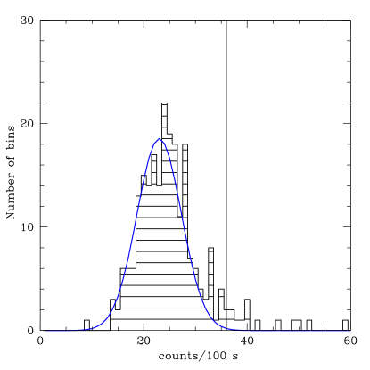
Figure 1.— The background counts distribution in the PN observation of Field 6. The solid line represents the best gaussian fit to the distribution. The continuous vertical line represents the adopted 3$\sigma$ cut above which the corresponding time intervals have been discarded.

In Fig. 1 an example of the application of this method to Field #6 is shown. Once the high energy flares were removed, the 0.3–10 keV background counts distribution was processed, with the same 3$\sigma$ clipping method, in order to remove times during which low energy particle flares were important. These flares are not easily detected in the 12–14 keV band. As a result of this selection process the average time lost due to particle flares was $<$20$\%$ and 2 observations were completely lost (see Hasinger et al., 2007).
An important feature observable in the background spectrum of both MOS and PN CCDs is the Al K$\alpha$ (1.48 keV) fluorescent emission. In the PN background two strong Cu lines are also present at $\sim$ 7.4 keV and $\sim$ 8.0 keV. Since these emission lines could affect the scientific results, the 7.2–7.6 keV and 7.8–8.2 keV energy bands in the PN and the 1.45–1.54 keV band (in PN and MOS) were excluded from the detectors events. Images were then created in the 0.5–2 keV, 2–4.5 keV and 4.5–10 keV energy bands with a pixel size of 4 arcsec. Single and double events were used to construct the PN images, while MOS images were created using all valid event patterns. Out-of-Time (OOT) events appear when a photon hits the CCD during the read-out process in the IMAGING mode. The result is that the x position of the event/photon is known, while the y position is unknown due to the readout and shifting of the charges at this time. For this reason artificial OOT event files were created. A new y coordinate is simulated by randomly shifting the event along the readout axis and performing the gain and CTI (charge transfer inefficiency) correction afterwards. For the PN, in full frame mode the OOT events constitute about 6.3$\%$ of the observing time. Those files were filtered in the same way as the event files and the produced images were subtracted from the event images. Images were then added in order to obtain PN+MOS mosaics. For each instrument and for each observation, spectrally weighted exposure maps were created using the SAS task eexpmap, assuming a power law model with photon index $\Gamma$=2.0 in the 0.5–2 keV band and $\Gamma$=1.7 in the 2–4.5 and 4.5–10 keV bands.

2.1. Astrometry correction

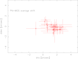
Figure 2.— Shift between the PN+MOS mosaic and the MEGACAM catalog for each pointing of the XMM-Newton COSMOS field.

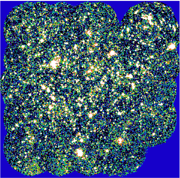
Figure 3.— Signal–to–noise ratio map in the 0.5–2 keV band of the XMM–Newton raster scan in the COSMOS field. The stretch of the color map corresponds to [-0.1$<$S/N$<$1 per pixel]. The scale has been chosen to enhance the SNR contrasts. If $S$ is the raw (sources + background) image and $B$ is the model background image, then the SNR map is obtained by $SNR=\frac{S-B}{\sqrt{S}}$. The image was smoothed with a gaussian filter with $\sigma$=2 pixels. Negative values are places where the measured background is smaller than the model background.

In order to correct the astrometry of our XMM–Newton  observations for each pointing and for each instrument, the produced X-ray source list (see next section) was compared with the MEGACAM catalog of the COSMOS field (Mc Cracken et al., 2007) including all the sources with I magnitudes in the range 18-23. In order to find the shift between the two catalogues, an optical-X-ray positional correlation was computed using the likelihood algorithm included in the SAS task eposcorr. This task uses in a purely statistical way all possible counterparts of an X-ray source in the field to determine the most likely coordinate displacement. This method is independent of actual spectroscopic identifications, but all post-facto checks using, for example, secure spectroscopic identifications, have demonstrated its reliability and accuracy. Using the magnitude range mentioned above, systematic effects introduced by bright stars and faint background objects are minimized. In the majority of the observations the shift between the three cameras turned out to be $<$ 1” (i.e. much smaller than the pixel size of the images used here ). Since the shift between the EPIC cameras is negligible, a correlation between the joint MOS+PN source list and the optical catalog was calculated to derive the astrometric correction. For the 23 pointings presented here, the shifts between the optical and X-ray catalog are never larger than 3$"$, with an average shift of the order of $\Delta\alpha\sim$1.4$"$ and $\Delta\delta\sim$-0.17$"$. The average displacement in the two coordinates between the PN+MOS mosaic X-ray positions and the MEGACAM catalog sources for each pointing of the XMM-COSMOS field is shown in Fig 2. The appropriate offset was applied to the event file of each pointing and images and exposure maps were then reproduced with the corrected astrometry.

3. EPIC source detection

Table 1Summary of source detection

Energy Band	$\Gamma$	ECF	Slim	N sources	Single detections
keV		cts s-1/10-11 erg cm-2 s-1	erg cm-2 s-1	All	Point-like
0.5–2	2.0	10.45	7.2$\times$10-16	1307	1281	661
2–4.5	1.7	1.52	4.0$\times$10-15	735	724	89
4.5–10	1.7	1.21	9.7$\times$10-15	187	186	3

3.1. Background modeling

In order to perform the source detection a sophisticated background modeling has been developed. In X-ray observations the background is mainly due to two components, one generated by undetected faint sources contributing to the cosmic X-ray background and one arising from soft protons trapped by the terrestrial magnetic field. For this reason two background templates were computed for each instrument and for each pointing, one for the sky (vignetted) background (Lumb et al., 2002) and one for instrumental and particles background (unvignetted). To calculate the normalizations of each template of every pointing, we first performed a wavelet source detection (see Finoguenov et al., 2007) without sophisticated background subtraction, then we excised the areas of the detector where a significant signal due to sources was detected. The residual area is split into two parts depending on the value of the effective exposure (i.e. higher and lower than the median value). Using the two templates, we calculate the coefficients of a system of two linear equations from which we obtain the normalizations of both:

$$AM^{1}_{v}+BM^{1}_{unv}=C^{1}$$ (1)

$$AM^{2}_{v}+BM^{2}_{unv}=C^{2}$$ (2)

where A and B are the normalization factors, M${}^{1,2}_{v}$ the vignetted templates in the region with effective exposure higher and lower than the median , M${}^{1,2}_{unv}$ the unvignetted templates and C^1,2 are the background counts in the two regions. The region with effective exposure lower than the median (i.e. high vignetting, $\gtrsim$7’ off-axis) is dominated by the instrumental background, while the region with higher effective exposure is dominated by the sky background. Therefore with this method we have the advantage of better fitting the two components of the background. The standard method for estimating the background, based on the spline functions used in the  XMM–Newton  pipelines, returned in our case significant residuals. The excellent result of this technique can be seen in the signal-to-noise (SNR) map in Fig 3: despite the significant variations in exposure time and average background level from pointing to pointing, a rather homogeneous signal–to–noise ratio is achieved across the whole mosaic. It is worth noting that also pixels with negative values are shown in the map; these are located where the background model is higher than the measured background.

3.2. Maximum likelihood detection

In each pointing the source detection was conducted on the combined images of the different instruments in the three energy bands mentioned above using the SAS tasks eboxdetect and emldetect. As a first step, the sliding cell detection algorithm eboxdetect was run on the images in the three energy bands. In this procedure source counts were collected in cells of 5$\times$5 pixels adopting a low threshold in the detection likelihood (i.e. likemin=4). The source list produced by eboxdetect was then used as input for emldetect. For all the sources detected with the sliding cell method this task performs a maximum likelihood PSF fit. In this way refined positions and fluxes for the sources were determined. Due to the particular pattern of our observations (see Hasinger et al., 2007), the same source could be detected in up to 4 different pointings. For this reason both eboxdetect and emldetect were run in raster mode. The source parameters (position and flux) were fitted simultaneously on all the observations where the source is observable, taking into account the PSF at the source position in each pointing. As likelihood threshold for the detection, we adopted the value det_ml=6. This parameter is related to the probability of a random Poissonian fluctuation having caused the observed source counts:

$$det\_ml=-lnP_{random}$$ (3)

In principle, the expected number of spurious sources could be estimated as the product of the probability for a random Poisson fluctuation exceeding the likelihood threshold times the number of statistically independent trials, N_trial. For a simple box detection algorithm N_trial would be approximately given by the number of independent source detection cells across the field of view. For the complex multi-stage source detection algorithm, like the one applied here, N_trial cannot be calculated analytically, but has to be estimated through Monte Carlo simulations. These simulations, which are discussed in Section 4, return a number of spurious sources of $\sim$2% at the likelihood level chosen. All the sources were fitted with a PSF template convolved with a beta model (Cavaliere & Fusco-Femiano, 1976). Sources which have a core radius significantly larger than the PSF are flagged as extended (ext parameter $>0$).

A total of 1307, 735 and 187 X-ray sources were detected in the three bands. Of these sources, twenty-six were classified as extended. The analysis of the X-ray extended sources in the COSMOS field is beyond the scope of this work; these sources are extensively discussed by Finoguenov et al. (2007). A total of 1281, 724 and 186 point-like sources were detected in the three bands down to limiting fluxes of 7.2$\times$10^-16 erg cm^-2 s^-1, 4.7$\times$10^-15 erg cm^-2 s^-1 and 9.7$\times$10^-15 erg cm^-2 s^-1 respectively. The minimum number of net counts for the detected sources is $\sim$21, 17 and 27 in the three bands, respectively. A total of 1390 independent point-like sources have been detected by summing the number of sources detected in each band but not in any softer energy band. The number of sources detected only in the 0.5–2 keV, 2–4.5 keV, 4.5–10 keV bands are 661, 89 and 3, respectively.

From the count rates in the 0.5–2 keV, 2–4.5 keV and 4.5–10 keV bands the fluxes were obtained in the 0.5–2 keV, 2–10 keV and 5–10 keV bands respectively using the energy conversion factors (ECF) listed in Table 1, together with a summary of the source detection. The ECF values have been computed using the most recent EPIC response matrices in the corresponding energy ranges. As a model, we assumed power-law spectra with N_H =2.6$\times$10²⁰ cm^-2, (corresponding to the average value of N_H over the whole COSMOS field (Dickey & Lockman, 1990)) and the same spectral indices used to compute the exposure maps without considering any intrinsic absorption (see Table 1). It is worth noting that the spectral indices and the absorptions of the individual sources can be significantly different from the average values assumed here. In particular Mainieri et al. (2007) found that the spectral indices $\Gamma$ of the XMM-COSMOS sources are in the range 1.5$\div$2.5, in the CDFS Tozzi et al. (2006) measured an average photon index $<\Gamma>\sim$1.75 and similar values were obtained by Kim et al. (2004) in the CHAMP survey. The mean spectrum assumed here is therefore consistent with the values measured up to now. By changing the spectral index of $\pm{0.3}$ the ECFs change of 2%, 12% and 4% in the 0.5–2 keV, 2–4.5 keV and 4.5–10 keV, respectively.

Figure 4.— The cumulative probability to detect a true source with det$\_$ml$>$6 in a circle of a given radius in the 0.5–2 ($continuous~{}line$), 2–4.5 ($dashed~{}line$) and 4.5–10 keV ($dashed-dotted~{}line$) energy bands. The 68%, 90% and 99% levels are plotted as horizontal lines.

4. Monte Carlo simulations

In order to properly estimate the source detection efficiency and biases, detailed Monte Carlo simulations were performed (see, e.g., Hasinger et al., 1993; Loaring et al., 2005). Twenty series of 23 XMM–Newton  images were created with the same pattern, exposure maps and background levels as the real data. The PSF of the simulated sources was constructed from the templates available in the XMM–Newton  calibration database. The sources were randomly placed in the field of view according to a standard 0.5-2 keV logN-logS distribution (Hasinger et al., 2005). This was then converted to a 2–4.5 keV and 4.5–10 keV logN-logS assuming that all the sources have the same intrinsic spectrum (a power-law with spectral index $\Gamma=1.7$). We then applied, to the simulated fields, the same source detection procedure used in the real data. Schmitt & Maccacaro (1986) showed that with the threshold adopted here for source detection, which corresponds roughly to the Gaussian 4.5-5$\sigma$, the distortion of the slope of the logN-logS due to Poissonian noise is $<$3$\%$ for a wide range of slopes. Therefore, the uncertainties introduced by using a single logN-logS as base for the simulations are negligible. A total of 30626, 13579 and 3172 simulated sources were detected in the 0.5–2 keV, 2–4.5 keV and 4.5–10 keV bands down to the same limiting fluxes of the observations. For every possible pair of input-output sources we computed the quantity

$$R^{2}=\left(\frac{x-x_{0}}{\sigma_{x}}\right)^{2}+\left(\frac{y-y_{0}}{\sigma_{y}}\right)^{2}+\left(\frac{S-S_{0}}{\sigma_{S}}\right)^{2},$$ (4)

where $x,y$ and $S$ are the position and flux of the detected source and $x_{0},y_{0}$ and $S_{0}$ are the corresponding values for all the simulated sources We then flag as the most likely associations those with the minimum value of $R^{2}$. The distribution of the positional offsets is plotted in Fig. 4 for each energy band analyzed.

Figure 5.— The ratio S_out/S_in as a function of the output detected flux in the 0.5–2 keV, 2–4.5 keV and 4.5–10 keV bands, respectively$Top~{}middle~{}and~{}bottom~{}panel$.

We find that 68% of the sources are detected within 2.1$"$, 1.3$"$ and 0.8$"$ in the 0.5–2 keV, 2–4.5 keV and 4.5–10 keV bands, respectively. Since the detection software fits the position of the source using the information available for the three bands together, we expect to be able to detect sources with an accuracy of the order of, or somewhat better than, that shown in Fig. 4. As in Loaring et al. (2005), we then define a cut-off radius $r_{cut}$ of 6$"$. Sources with a displacement larger than $r_{cut}$ from their input counterpart are classified as spurious. These account for 2.7%, 0.5%, 0.6% of the total number of sources in the 0.5–2 keV, 2–4.5 keV and 4.5–10 keV bands, respectively. Source confusion occurs when two or more sources fall in a single resolution element of the detector and result as a single detected source with an amplified flux. In order to determine the influence of the source confusion we adopted the method described in Hasinger et al. (1998). We define as $"confused"$ sources those for which $S_{out}/(S_{in}+3*\sigma_{out})>1.5$ (where $\sigma_{out}$ is the 1$\sigma$ error on the output flux). The fraction of $"confused"$ sources is 0.8$\%$, 0.15$\%$ and $<$0.1$\%$ in the 0.5–2 keV, 2–4.5 keV and 4.5–10 keV bands, respectively.
The photometry was also tested; the ratio of output to input fluxes in the simulation is plotted in Fig.5.

At bright fluxes this ratio is consistent with one, while at fainter fluxes the distribution of $S_{out}/S_{in}$ becomes wider, mainly because of increasing errors, and skewed toward values greater than one. This skewness of the distribution can be explained mainly by two effects: a) source confusion and b) Eddington Bias (Eddington, 1940). While source confusion, as defined above, affects only a small fraction of the sources, the Eddington bias results in a systematic upward offset of the detected flux. The magnitude of this effect depends on the shape of the logN-logS distribution and the statistical error on the measured flux. Since there are many more faint than bright sources, uncertainties in the measured flux will result in more sources being up-scattered than down-scattered. Together with this, the fact that in the 4.5–10 keV band we are sampling a flux region in which the logN-logS is steeper than in the other bands (see Section 5), explains why such an effect is more evident in the 4.5–10 keV band.

Besides assessing the reliability of our source detection procedure, one of the aims of these simulations is to provide a precise estimation of the completeness function of our survey, known also as sky coverage. We constructed our sky-coverage ($\Omega$) vs. flux relation by dividing the number of detected sources by the number of input sources as a function of the flux and rescaling it to the sky simulated area. Having analyzed the simulations with the same procedure adopted for the analysis of the data, this method ensures that when computing the source counts distribution (see next section) all the observational biases are taken into account and corrected. The $\Omega$ vs. flux relation relative to the 0.5–2 keV, 2–10 keV and 5–10 keV bands is plotted in fig. 6. The total sky area is 2.03 deg² and it is completely observable down to fluxes of $\sim$0.3, 1.3 and 2$\times$10^-14 erg cm^-2 s^-1 in the three bands, respectively. The sky coverage drops to 0 at limiting fluxes of $\sim$7$\times$10^-16 erg cm^-2 s^-1, $\sim$4$\times$10^-15 erg cm^-2 s^-1and $\sim$9$\times$10^-15 erg cm^-2 s^-1, in the 0.5–2 keV, 2–10 keV and 5–10 keV bands, respectively.

5. Source counts

Figure 6.— The sky coverage vs. flux relation in the 0.5-2, 2-10 and 5-10 keV energy bands (respectively continuous, dashed and dash-dotted line), resulting from the simulations described in the text.

Table 2Cumulative number counts

log(S)	$\Omega$	N($>$S)
erg cm-2 s-1	deg2	deg-2
0.5–2 keV
-13.0	2.03	4.5$\pm{1.5}$
-13.5	2.03	18.8$\pm{3.1}$
-14.0	2.03	105.2$\pm{7.0}$
-14.5	2.03	327.0$\pm{12.7}$
-15.0	0.58	790$\pm{23.3}$
-15.1	0.12	931$\pm{53.0}$
2–10 keV
-13.0	2.03	8.6$\pm{2.0}$
-13.5	2.03	57.0$\pm{5.3}$
-14.0	1.40	258.9$\pm{11.6}$
-14.3	0.13	600.1$\pm{34.2}$
5–10 keV
-13.5	2.03	21.3$\pm{3.2}$
-14.0	0.35	111$\pm{11.0}$

Once the sky coverage is known, the cumulative source number counts can be easily computed using the following equation:

$$N(>S)=\sum_{i=1}^{\it N_{S}}\frac{1}{\Omega_{i}}deg^{-2},$$ (5)

where $N_{S}$ is the total number of detected sources in the field with fluxes greater than $S$ and $\Omega_{i}$ is the sky coverage associated with the flux of the i^th source. The variance of the source number counts is therefore defined as:

$$\sigma_{i}^{2}=\sum_{i=1}^{\it N_{S}}\left(\frac{1}{\Omega_{i}}\right)^{2}.$$ (6)

Source number counts are reported in Table 2. The cumulative number counts, normalized to the Euclidean slope (multiplied by S^1.5), are shown in Figures 7, 8 and 9,

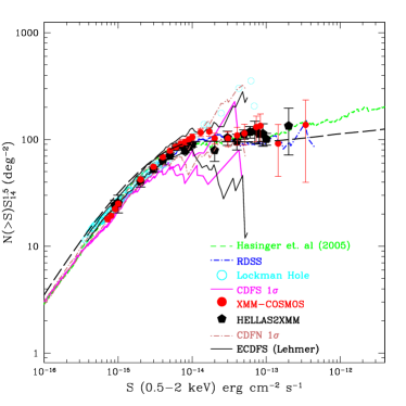
Figure 7.— The 0.5-2 keV logN-logS of the XMM-COSMOS ($red~{}dots$) sources compared with the ROSAT medium sensitivity survey (Hasinger et al., 1993) ($blue~{}dot~{}dashed~{}line$), combined ROSAT, XMM–Newton , Chandra (Hasinger et al., 2005) ($green~{}dashed~{}line$), the Chandra deep field south 1$\sigma$ error tie (Rosati et al., 2002) ($magenta~{}continuous~{}line$), the Chandra deep field north 1$\sigma$ error tie (Bauer et al., 2004) ($pink~{}dot-dashed~{}line$), the 100 ks of the XMM–Newton  Lockman hole  (Hasinger et al., 2001) ($cyan~{}circles$), the HELLAS2XMM (Baldi et al., 2002) ($black~{}pentagons$) and the extended CDFS (Lehmer et al., 2005) ($black~{}continuous~{}line$) surveys. The overlayed black-dashed line represents the logN-logS predicted by the model of Gilli, Comastri & Hasinger (2006). The source number counts are plotted scaled by S^1.5 in order to highlight the deviation from the Euclidean behavior.

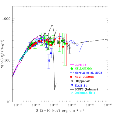
Figure 8.— The 2-10 keV logN-logS of the XMM-COSMOS ($red~{}dots$) sources compared with Chandra, XMM–Newton  and ASCA ($blue~{}dashed~{}line$) (Moretti et al., 2003), HELLAS BeppoSAX (Giommi et al., 2000) ($black~{}hexagons$) the Chandra deep field south 1$\sigma$ error tie (Rosati et al., 2002) ($magenta~{}continuous~{}line$), the HELLAS2XMM ($green~{}pentagons$) (Baldi et al., 2002), the ELAIS S1 ($blue~{}stars$) (Puccetti et al., 2006), the extended CDFS (Lehmer et al., 2005) 1$\sigma$ error tie ($black~{}continuous~{}line$) and the 100 ks of the Lockman hole ($cian~{}open~{}circles$) (Hasinger et al., 2001). The overlayed black-dashed line represents the logN-logS predicted by the model of Gilli, Comastri & Hasinger (2006). The source number counts are plotted scaled by S^1.5 in order to highlight the deviation from the Euclidean behavior.

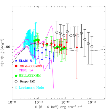
Figure 9.— The 5-10 keV logN-logS of the XMM-COSMOS ($red~{}dots$) sources compared with the HELLAS2XMM (Baldi et al., 2002) ($green~{}pentagons$), the Chandra deep field south 1$\sigma$ error tie (Rosati et al., 2002) ($magenta~{}continuous~{}line$) , the HELLAS-BeppoSAX data from Fiore et al. (2001) ($black~{}hexagons$), the ELAIS S1 ($blue~{}stars$) (Puccetti et al., 2006) and the 100 ks of the Lockman Hole ($cyan~{}open~{}circles$) (Hasinger et al., 2001). The overlayed black-dashed line represents the logN-logS predicted by the model of Gilli, Comastri & Hasinger (2006). The source number counts are plotted scaled by S^1.5 in order to highlight deviation from the Euclidean behavior.

for the 0.5–2 keV, 2–10 keV and 5–10 keV energy ranges, respectively. With such a representation, the deviations from the Euclidean slope are clearly evident as well as the flattening of the counts towards faint fluxes. Source counts are compared with the findings of other deep and shallow surveys collected from the literature. The plotted reference results were selected in order to sample a flux range as wide as possible and at the same time to keep the plots as clear as possible. As discussed in the previous section, the sky coverage $\Omega$ was derived from realistic Monte Carlo simulations and therefore no further correction for the Eddington Bias is required.

In order to parameterize our relations, we performed a maximum likelihood fit to the unbinned differential counts. We assumed a broken power-law model for the 0.5–2 keV and 2–10 keV bands:

$$n(S)=\frac{dN}{ds}=\left\{\begin{array}[]{ll}A\,S^{-\alpha_{1}}&S>S_{b}\\ B\,S^{-\alpha_{2}}&S\leq S_{b},\\ \end{array}\right.$$ (7)

where $A=B\,S_{b}^{\alpha_{1}-\alpha_{2}}$ is the normalization, $\alpha_{1}$ is the bright end slope, $\alpha_{2}$ the faint end slope, $S_{b}$ the break flux, and $S$ the flux in units of 10^-14 erg cm^-2 s^-1 . Notice that using the maximum likelihood method, the fit is not dependent on the data binning and therefore we can make full use of the whole dataset. Moreover, the normalization $A$ is not a parameter of the fit, but it is obtained by imposing the condition that the number of expected sources from the best fit model is equal to the total observed number. In the 0.5–2 keV energy band the best fit parameters are $\alpha_{1}$=2.60${}^{+0.15}_{-0.18}$, $\alpha_{2}$=1.65$\pm{0.05}$, $S_{b}$=1.55${}^{+0.28}_{-0.24}$ $\times$10^-14 erg cm^-2 s^-1  and $A$=123. Translating this value of the normalization to that for the cumulative distribution at 2$\times$10^-15 erg cm^-2 s^-1 , which is usually used in the literature for Chandra surveys, we obtain $A_{15}\sim$450 which is fully consistent with most of previous works where a fit result is presented (Hasinger et al., 1993; Mushotzky et al., 2000; Hasinger et al., 2001; Baldi et al., 2002; Rosati et al., 2002; Bauer et al., 2004; Kim et al., 2004; Hasinger et al., 2005; Kenter et al., 2005), but significantly lower than that found in the CLASXS survey (Yang et al., 2004). In the 2–10 keV band the best fit parameters are $\alpha_{1}$=2.43$\pm{0.10}$, $\alpha_{2}$=1.59$\pm{0.33}$, $S_{b}$=1.02${}^{+0.25}_{-0.19}$ $\times$10^-14 erg cm^-2 s^-1  and $A$=266. The latest value translates into $A_{15}\sim$1250. Also in this band, our results are in agreement with previous surveys within 1$\sigma$, with the exception of the CLASXS survey which is $\sim$30% higher in this band (Yang et al., 2004). In the 5–10 keV energy bands, where the differential counts do not show any evidence for a break in the sampled flux range, we assumed a single power-law model of the form:

$$n(S)=\frac{dN}{ds}=A\,S^{-\alpha_{1}},$$ (8)

for which the best fit parameters are found to be $A$=102 and $\alpha_{1}$=2.36$\pm{0.1}$.

In the soft 0.5-2 keV (Fig. 8) energy range a visual inspection of the various datasets suggests a remarkably good agreement between XMM-COSMOS and literature data.

In the 2–10 keV band the XMM-COSMOS counts bridge the gap between deep field observations (Rosati et al., 2002) and shallower large area BeppoSAX (Giommi et al., 2000) and XMM–Newton surveys (Baldi et al., 2002). At relatively bright fluxes ($>10^{-14}$ erg cm^-2 s^-1) the XMM-COSMOS logN–logS nicely matches previous measurements, though providing a much more robust estimate of the source counts thanks to the much smaller statistical errors.

A major step forward in the determination of X–ray source counts is achieved in the 5–10 keV band, where the previously existing data from different surveys show very significant differences. Thanks to XMM–COSMOS, a solid measure of the hard-X logN–logS in the flux interval 10^-14 – 10^-13 erg cm^-2 s^-1  is obtained for the first time. From Fig. 9 we notice that the normalization of the XMM–COSMOS logN–logS is slightly higher than ($\sim$10%), although consistent at 1$\sigma$ with, that measured by Chandra while, ELAIS S1 (Puccetti et al., 2006) source counts are 30% lower. However, in the overlapping flux range the latter is characterized by large errors due to the small number of relatively bright sources in the Chandra deep fields. Interestingly enough, the XMM–COSMOS counts match nicely, with smaller errors, those of the wide area HELLAS2XMM survey (Baldi et al. 2002), while the pioneering measurements of BeppoSAX (Fiore et al., 2001) are systematically higher than the counts from XMM-COSMOS.

5.1. Resolved fraction of the X-ray background

One of the main aims of XMM-COSMOS with its large and medium–deep coverage, is to provide a solid census of the X-ray source population to be compared with observations and models of AGN evolution. According to recent synthesis models (see e.g.; Comastri et al., 1995; Gilli, Comastri & Hasinger, 2006; Worsley et al., 2005) a high fraction of heavily obscured AGN is necessary to explain the spectral shape and the intensity of the X-ray background (XRB). We examine therefore which fraction of XRB is resolved into discrete sources in our survey.

As a first test, we computed the flux which XMM-COSMOS itself resolves into discrete sources by summing their fluxes weighted on the sky coverage in the 0.5–2 keV, 2–10 keV and 5-10 keV energy bands. As in Worsley et al. (2005) we used as reference value of the normalization at 1 keV of the XRB spectrum that of De Luca & Molendi (2004) which assumes that the spectral shape in the 1-10 keV band is a power-law with spectral index $\Gamma$=1.4 and a normalization at 1keV of 11.6 keV cm^-2 s^-1 keV^-1. The latter value corresponds to a flux of 0.80, 2.31 and 1.27$\times 10^{-11}$ erg cm^-2 s^-1 deg^-2  in the 0.5–2 keV, 2–10 keV and 5-10 keV energy bands, respectively. In the 0.5–2 keV band we measure a contribution of the sources to the XRB which corresponds to a normalization at 1 keV of 0.49$\pm{0.08}\times 10^{-11}$ erg cm^-2 s^-1 deg^-2. The corresponding values in the 2–10 keV and 5–10 keV bands are 0.92$\pm{0.22}\times 10^{-11}$ erg cm^-2 s^-1 deg^-2  and 0.28$\pm{0.15}\times 10^{-11}$ erg cm^-2 s^-1 deg^-2. Therefore XMM-COSMOS resolves by itself $\sim$65$\%$, $\sim$40$\%$ and $\sim$22$\%$ of the XRB into discrete sources in the 0.5–2 keV, 2–10 keV and 5–10 keV energy bands, respectively. It is worth noticing that the flux measured by De Luca & Molendi (2004) is the highest measured in literature in the 1–10 keV energy range (see e.g. Gilli, Comastri & Hasinger, 2006, for a complete collection). It is also worth noticing that we computed the fraction of resolved XRB by assuming that all the sources have the same spectrum. Therefore, in our estimate, effects due to the broad absorption and spectral index distributions of AGNs are not included.

In Figs. 7, 8 and 9 we compared our logN-logS to those predicted by the recent XRB model of Gilli, Comastri & Hasinger (2006). This model makes use of the most recent observational constraints on the AGN populations and includes a conspicuous fraction of Compton thick AGN which, however, are not expected to significantly contribute to the XMM-COSMOS counts. In the 0.5–2 keV band a direct comparison of our data with the model shows a 1$\sigma$ agreement at the bright end. At the faint end the model predicts a slightly higher normalization when compared to most of the plotted data, including ours. A similar behavior is observed in the 2–10 keV band. It is worth noticing that in the model the average unabsorbed power-law spectral index of the sources is $<\Gamma>\sim$1.8 in the flux interval sampled by XMM-COSMOS (see Fig. 19 in Gilli, Comastri & Hasinger (2006)). Since in our data analysis we assumed $<\Gamma>$=1.7 we expect in this band a slight ($\sim$10%) underestimation of the fluxes when compared to those of the model. This effect is almost negligible (i.e. $<$5%) in the other bands investigated here.

By integrating our best fit 2–10 keV logN-logS between infinite and zero, and assuming that the slope of the ”real” logN-logS remains constant down to low fluxes, we estimated the total contribution of AGNs to the XRB. We predict a total flux of AGNs in the XRB of 1.25$\times 10^{-11}$ erg cm^-2 s^-1 deg^-2. This value is $\sim$40% lower than that measured by De Luca & Molendi (2004), and $\sim$ 25% smaller than those obtained by integration the model logN-logS of Gilli, Comastri & Hasinger (2006) which predicts a flux of $\sim$1.66$\times 10^{-11}$ erg cm^-2 s^-1 deg^-2. This discrepancy between our predicted flux and that of Gilli, Comastri & Hasinger (2006), could arise by the fact that, in our measurement, we consider that all the sources have the same spectrum and from statistical uncertainty of the logN-logS parameters. By assuming an average spectral index $<\Gamma>$=1.4 for all our sources, we obtain a value for the total flux of the AGNs of $\sim$1.48$\times 10^{-11}$ erg cm^-2 s^-1 deg^-2  which is consistent, within the statistical uncertanties, with the prediction of the model. Considering the total flux of the XRB predicted by the model and our estimate from the logN-logS distributions, in the 2–10 keV band, XMM-COSMOS resolves the $\sim$55–65% of the total flux of the XRB into discrete sources.

It is interesting to observe how in the 5–10 keV band our data are in good agreement with the prediction of the model. This result is particularly important since in this band it is expected the major contribution of highly absorbed AGN, which are an important ingredient of the XRB models. A detailed analysis of the spectral properties of the brightest X-ray sources in XMM-COSMOS is presented by Mainieri et al. (2007).

6. Sample variance

The amplitude of source counts distributions varies significantly among different surveys (see e.g. Yang et al., 2003; Cappelluti et al., 2005, and references therein). This ”sample variance”, can be explained as a combination of Poissonian variations and effects due to the clustering of sources (Peebles, 1980; Yang et al., 2003). The variance of counts in cells for sources which are angularly correlated can be obtained with:

$$<(N-\mathcal{N}\Omega)^{2}>=\mathcal{N}\Omega+\mathcal{N}^{2}\,\int\,d\Omega_{1}\,d\Omega_{2}w(\theta_{1,2})$$ (9)

where $\mathcal{N}$ is the mean density of objects in the sky, $\Omega$ is the cell size, and $w(\theta_{1,2})$ is the angular two–point correlation function. The first term of Eq. 9 is the Poissonian variance and the second term is introduced by the large scale structure. In order to determine whether the differences observed in the source counts of different surveys could arise from the clustering of X-ray sources, we estimated the amplitude of the fluctuations from our data, by producing subsamples of our survey with areas comparable to those of. e.g., Chandra surveys.
The XMM-COSMOS field and the Monte Carlo sample fields of Section 4 were divided in 4,9,16 and 25 square boxes. Making use of the 0.5–2 keV energy band data, we computed for each subfield, the ratio of the number of real sources to the number of random sources. In order to prevent incompleteness artifacts, we conservatively cut the limiting flux of the random and data sample to 5$\times$10^-15 erg cm^-2 s^-1. At this flux our survey is complete over the entire area. In order to avoid artifacts introduced by the missing pointings in the external part of the field of view, we concentrated our analysis to the central 80${}^{\prime}\times$80^′.

Figure 10.— The counts in cell fluctuations within the XMM-COSMOS field. The data are normalized to a random distributed field in boxes of 40’,26’,20’ and 16’ of side, respectively. The dashed lines represent the 1$\sigma$ expected fluctuation.

In Fig.10 we plot the ratio of the data to the random sample as a function of the size of the cells under investigation. The measured fractional standard deviations of the sample is reported in Table 3. Using Eq. 9 we computed the expected amplitude of source counts fluctuations with $w(\theta_{1,2})$ taken from Miyaji et al. (2007). They computed the X-ray two–point correlation function in the XMM-COSMOS field and detected clustering signal with angular correlation length $\theta_{0}$ $\sim$1.9$"$ $\sim$0.8$"$ and $\sim$6$"$ in the 0.5–2 keV, 2–4.5 keV and 4.5–10 keV band, respectively. The observed slope is $\gamma$=1.8 in all the energy bands.

The predicted fractional standard deviations are therefore 0.13, 0.19, 0.23 and 0.28 on scales of 0.44 deg², 0.19 deg², 0.11 deg² and 0.07 deg², respectively. These values are in good agreement with those observed in the sub-samples of our dataset as shown by the value of the fitted $\chi^{2}$ to the counts in cell fluctuations (see Table 3). As shown in Table 3, at this limiting flux and on the areas considered here the main contribution to the source counts fluctuations is from the Poissonian noise. At the flux limit assumed here, the ratio $\sigma_{cl}$/$\sigma_{p}$ increases from $\sim$0.5 on the smallest scale (16 x 16 arcmin) to $\sim$0.85 on the largest scale (40 x 40 arcmin). This ratio scales as:

$$\sigma_{cl}/\sigma_{p}\propto\mathcal{N}^{0.5}\theta_{0}^{(\gamma-1)/2}a^{(3-\gamma)/2},$$ (10)

where $\mathcal{N}$ deg^-2 is the surface density of the sources, $\theta_{0}$ (deg) is the angular correlation length and $a$ (deg) is the size of the cell. In order to estimate at which flux limit fluctuations introduced by the large scale structure are predominant, we estimate that $\sigma_{cl}$/$\sigma_{p}$ would be $\sim$1 on the smallest scale, corresponding to a Chandra ACIS field of view (16 x 16 arcmin) at a surface density of the order of $\sim$900 deg^-2, corresponding to a 0.5-2 keV flux S$\sim$ 8$\times$10^-16 erg cm^-2 s^-1. At even fainter fluxes the dominant contribution to the total expected source counts fluctuations on this area ($\sigma_{exp}$ ) comes from the large scale structure, therefore the contribution of statistical fluctuations becomes less important. With the same procedure, we can estimate the total expected fluctuations ($\sigma_{exp}$) and the relative importance of $\sigma_{p}$ and $\sigma_{cl}$ also for the hard band (5-10 keV), even if in this band we do not have enough statistics to divide our field in sub-samples. Using the formal best fit for $\theta_{0}$ in this band found by Miyaji et al. (2007) ($\theta_{0}$=6$"$), we find that at the faintest 5-10 keV flux (S$\sim$10^-14 erg cm^-2 s^-1) sampled by the XMM-COSMOS survey ($\mathcal{N}\sim$ 110 deg^-2 ) the ratio $\sigma_{cl}$/$\sigma_{p}$ is smaller than one on all the four scales here analyzed, with a total expected standard deviation of the fluctuations ranging from $\sim$0.20 on the largest scale to $\sim$0.40 on the smallest scale. These values for $\sigma_{exp}$ are significantly larger than those shown in Table 3 for the soft band, because in the hard band the surface density of sources is lower and the angular correlation length is higher than in the soft band.

This analysis is at least qualitatively consistent with Figures 8 and 10, which show a significantly larger dispersion in the data from different surveys in the hard band than in the soft band. Moreover, the results here discussed are also consistent with the observed fluctuations in the deep Chandra fields (see, for example, Bauer et al. 2004). Large area, moderately deep surveys like XMM-COSMOS are needed to overcome the problem of low counting statistics, typical of deep pencil beam surveys, and, at the same time, to provide a robust estimate of the effect of large scale structure on observed source counts.

As a final consideration, we tried to compute the expected intrinsic variance of XMM-COSMOS. This estimate must be made with care since we have only one sample on this scale. Assuming that the angular correlation function of Miyaji et al. (2007) was universal, the residual uncertainties on the source counts are estimated to be $<$5-6% in the 0.5–2 keV and 2–10 keV bands, and of the order of the 10% in the 5–10 keV band.

Table 3 Summary of the 0.5–2 keV sample variance in the COSMOS field. Prediction and observation at a flux limit S_lim=5$\times$10^-15 erg cm^-2 s^-1

Area	$\sigma_{obs}$	$\sigma_{p}$	$\sigma_{cl}$	$\sigma_{exp}$	$\chi^{2}$/d.o.f.
arcmin2
40${}^{\prime}\times$40′	0.09$\pm{0.04}$	0.10	0.09	0.13	4.21/3
26${}^{\prime}\times$26′	0.20$\pm{0.05}$	0.15	0.10	0.19	8.93/8
20${}^{\prime}\times$20′	0.21$\pm{0.04}$	0.20	0.11	0.23	16.63/15
16 ${}^{\prime}\times$16′	0.24$\pm{0.02}$	0.25	0.12	0.28	25.15/24

.

7. Summary

The data analysis of the first run of observations of the XMM-Newton COSMOS wide field survey has been presented. A total of 1390 point-like sources are detected on a contiguous area of about 2 deg² down to fluxes of 7.2$\times$10^-16 erg cm^-2 s^-1, 4.0$\times$10^-15 erg cm^-2 s^-1and 9.7$\times$10^-15 erg cm^-2 s^-1in the 0.5–2 keV, 2–10 keV and 5–10 keV energy bands, respectively. The detection procedure was tested through Monte Carlo simulations which confirmed the high level of accuracy in the determination of the source properties (aperture photometry and positioning) and allowed us to keep statistical biases under control.

A robust estimate of X–ray source counts at both soft and hard energies, obtained thanks to the large number of sources detected in the XMM–COSMOS survey, is presented in this paper. The differential logN–logS was fitted with a broken power-law model in the 0.5–2 keV and 2–10 keV energy bands, and with a single power-law model in the 5–10 keV energy band. In the soft 0.5–2 keV band, already extensively covered by ROSAT, XMM–Newton and Chandra surveys over a range of fluxes encompassing those sampled by the COSMOS survey, our results are in excellent agreement with previous analysis (see Fig 7), providing an independent evidence of the validity of our data analysis procedure.

The large number of X–ray sources of the COSMOS survey allowed us to constrain with unprecedented accuracy the logN-logS parameters in the 2–10 and 5–10 keV energy ranges over a range of fluxes which were previously poorly constrained. Most importantly, in the hard 5–10 keV band, we were able to fill the gap between the deep Chandra surveys in the CDFS and CDFN and shallower large area surveys. The deviations from other surveys, which are, however, less than 30%, have been explained in terms of low counting statistics of pencil beam surveys, and partially by the effect of large scale structure. The major step forward in the determination of hard X–ray source counts achieved thanks to the XMM–COSMOS survey will provide an important reference point for the study of the AGN demography and evolution especially with applications to obscured AGN. More specifically, the evolutionary properties of the obscured AGN can be tightly constrained, since they are indeed very sensitive, according to the most recent model of the X–ray background (Gilli, Comastri & Hasinger 2006), to the shape of the hard X–ray source counts around the break flux, which is precisely where the COSMOS data play a key role. In this context, we compared our results to the most recent predictions of the model by Gilli, Comastri & Hasinger (2006), finding a remarkable agreement between data and model.

The second pass of the XMM–Newton  observations in the COSMOS field (600 ks) has already started, and is expected to significantly increase the total number of X–ray sources. The results of the full XMM–COSMOS survey including the complete (AO3+AO4) source catalogue will be the subject of a future paper. It is anticipated that, when completed, the XMM–COSMOS survey will provide a number of X–ray sources over a large enough contiguous area and down to moderately deep fluxes that it will make possible the study of AGN evolution and their connection with the large scale structure in which they reside with unprecedented detail. The COSMOS field has been granted 1.8 Msec observation with Chandra in its central square degree (C-COSMOS, P.I. Martin Elvis). The joint Chandra and XMM–Newton  observation will provide an unprecedented lab for AGN physics.

References

- Baldi et al. (2002) Baldi, A., Molendi, S., Comastri, A., Fiore, F., Matt, G., & Vignali, C. 2002, ApJ, 564, 190
- Bauer et al. (2004) Bauer, F. E., Alexander, D. M., Brandt, W. N., Schneider, D. P., Treister, E., Hornschemeier, A. E., & Garmire, G. P. 2004, AJ, 128, 2048
- Brandt & Hasinger (2005) Brandt, W. N., & Hasinger, G. 2005, ARA&A, 43, 827
- Brunner et al. (2006) Brunner, A. et al. 2006, A&A, submitted
- Brusa et al. (2007) Brusa, M. et al. 2007, ApJS, this volume
- Cappelluti et al. (2005) Cappelluti, N., Cappi, M., Dadina, M., Malaguti, G., Branchesi, M., D’Elia, V., & Palumbo, G. G. C. 2005, A&A, 430, 39
- Cappelluti et al. (2006) Cappelluti, N., Boehringer, H., Schuecker, P., Pierpaoli, E., Mullis, C. R., Gioia, I. M., & Henry, J. P. 2006, accepted by A&A, ArXiv Astrophysics e-prints, arXiv:astro-ph/0611553
- Cappi et al. (2001) Cappi, M., et al. 2001, ApJ, 548, 624
- Cavaliere & Fusco-Femiano (1976) Cavaliere, A., & Fusco-Femiano, R. 1976, A&A, 49, 137
- Comastri et al. (1995) Comastri, A., Setti, G., Zamorani, G., & Hasinger, G. 1995, A&A, 296, 1
- Dickey & Lockman (1990) Dickey, J. M., & Lockman, F. J. 1990, ARA&A, 28, 215
- Della Ceca et al. (2004) Della Ceca, R., et al. 2004, A&A, 428, 383
- De Luca & Molendi (2004) De Luca, A., & Molendi, S. 2004, A&A, 419, 837
- Eddington (1940) Eddington, A. S., Sir 1940, MNRAS, 100, 354
- Finoguenov et al. (2007) Finoguenov, A. et al. 2007, ApJS, this volume
- Fiore et al. (2001) Fiore, F., et al. 2001, MNRAS, 327, 771
- Fiore et al. (2003) Fiore, F., et al. 2003, A&A, 409, 79
- Giacconi & Zamorani (1987) Giacconi, R., & Zamorani, G. 1987, ApJ, 313, 20
- Giacconi et al. (2001) Giacconi, R., et al. 2001, ApJ, 551, 624
- Gilli et al. (2003) Gilli, R., et al. 2003, ApJ, 592, 721
- Gilli, Comastri & Hasinger (2006) Gilli, R., Comastri, A. & Hasinger, G. 2006, A&A, in press, astro-ph/0610939
- Giommi et al. (2000) Giommi, P., Perri, M., & Fiore, F. 2000, A&A, 362, 799
- Green et al. (2004) Green, P. J., et al. 2004, ApJS, 150, 43
- Hasinger et al. (1993) Hasinger, G., Burg, R., Giacconi, R., Hartner, G., Schmidt, M., Trumper, J., & Zamorani, G. 1993, A&A, 275, 1
- Hasinger et al. (1998) Hasinger, G., Burg, R., Giacconi, R., Schmidt, M., Trumper, J., & Zamorani, G. 1998, A&A, 329, 482
- Hasinger et al. (2001) Hasinger, G., et al. 2001, A&A, 365, L45
- Hasinger et al. (2005) Hasinger, G., Miyaji, T., & Schmidt, M. 2005, A&A, 441, 417
- Hasinger et al. (2007) Hasinger, G. et al. 2007, ApJS, this volume
- Henry & Briel (1991) Henry, J. P., & Briel, U. G. 1991, A&A, 246, L14
- Johnson et al. (2003) Johnson, O., Best, P. N., & Almaini, O. 2003, MNRAS, 343, 924
- Kenter et al. (2005) Kenter, A., et al. 2005, ApJS, 161, 9
- Kim et al. (2004) Kim, D.-W., et al. 2004, ApJ, 600, 59
- La Franca et al. (2005) La Franca, F., et al. 2005, ApJ, 635, 864
- Lehmer et al. (2005) Lehmer, B. D., et al. 2005, ApJS, 161, 21
- Loaring et al. (2005) Loaring, N. S., et al. 2005, MNRAS, 362, 1371
- Lumb et al. (2002) Lumb, D. H., Warwick, R. S., Page, M., & De Luca, A. 2002, A&A, 389, 93
- Maccacaro et al. (1988) Maccacaro, T., Gioia, I. M., Wolter, A., Zamorani, G., & Stocke, J. T. 1988, ApJ, 326, 680
- Mainieri et al. (2007) Mainieri, V., et al. 2007, ApJS, this volume
- Mc Cracken et al. (2007) Mc Cracken, et al. 2007, ApJS, this volume
- Miyaji et al. (2000) Miyaji, T., Hasinger, G., & Schmidt, M. 2000, A&A, 353, 25
- Miyaji et al. (2007) Miyaji, T., et al. 2007, ApJS, this volume
- Moretti et al. (2003) Moretti, A., Campana, S., Lazzati, D., & Tagliaferri, G. 2003, ApJ, 588, 696
- Murray et al. (2005) Murray, S. S., et al. 2005, ApJS, 161, 1
- Mushotzky et al. (2000) Mushotzky, R. F., Cowie, L. L., Barger, A. J., & Arnaud, K. A. 2000, Nature, 404, 459
- Nandra et al. (2005) Nandra, K., et al. 2005, MNRAS, 356, 568
- Peebles (1980) Peebles, P. J. E. 1980, The large-scale structure of the universe (Princeton, N.J., Princeton University Press)
- Puccetti et al. (2006) Puccetti et al. 2006, A&A, 457, 501
- Rosati et al. (2002) Rosati, P., et al. 2002, ApJ, 566, 667
- Ruderman & Ebeling (2005) Ruderman, J. T., & Ebeling, H. 2005, ApJ, 623, L81
- Schmitt & Maccacaro (1986) Schmitt, J. H. M. M., & Maccacaro, T. 1986, ApJ, 310, 334
- Scoville et al. (2007) Scoville, N.Z. et al., 2007, ApJS this volume
- Spergel et al. (2003) Spergel, D. N., et al. 2003, ApJS, 148, 175
- Tozzi et al. (2006) Tozzi, P., et al. 2006, A&A, 451, 457
- Ueda et al. (1999) Ueda, Y., et al. 1999, ApJ, 518, 656
- Ueda et al. (2003) Ueda, Y., Akiyama, M., Ohta, K., & Miyaji, T. 2003, ApJ, 598, 886
- Virani et al. (2006) Virani, S. N., Treister, E., Urry, C. M., & Gawiser, E. 2006, AJ, 131, 2373
- Yang et al. (2003) Yang, Y., Mushotzky, R. F., Barger, A. J., Cowie, L. L., Sanders, D. B., & Steffen, A. T. 2003, ApJ, 585, L85
- Yang et al. (2004) Yang, Y., Mushotzky, R. F., Steffen, A. T., Barger, A. J., & Cowie, L. L. 2004, AJ, 128, 1501
- Yang et al. (2006) Yang, Y., Mushotzky, R. F., Barger, A. J., & Cowie, L. L. 2006, ApJ, 645, 68
- Worsley et al. (2005) Worsley, M. A., et al. 2005, MNRAS, 357, 1281