Properties of Ellipticity Correlation with Atmospheric Structure from Gemini South

Abstract

Cosmic shear holds great promise for a precision independent measurement of $\Omega\rm_{m}$, the mass density of the universe relative to the critical density. The signal is expected to be weak, so a thorough understanding of systematic effects is crucial. An important systematic effect is the atmosphere: shear power introduced by the atmosphere is larger than the expected signal. Algorithms exist to extract the cosmic shear from the atmospheric component, though a measure of their success applied to a range of seeing conditions is lacking.

To gain insight into atmospheric shear, Gemini South imaging in conjunction with ground condition and satellite wind data were obtained. We find that under good seeing conditions Point-Spread-Function (PSF) correlations persist well beyond the separation typical of high-latitude stars. Under these conditions, ellipticity residuals based on a simple PSF interpolation can be reduced to within a factor of a few of the shot-noise induced ellipticity floor. We also find that the ellipticity residuals are highly correlated with wind direction. Finally, we correct stellar shapes using a more sophisticated procedure and generate shear statistics from stars. Under all seeing conditions in our data set the residual correlations lie everywhere below the target signal level. For good seeing we find that the systematic error attributable to atmospheric turbulence is comparable in magnitude to the statistical error (shape noise) over angular scales relevant to present lensing surveys.

1 Introduction

Weak gravitational lensing is a powerful and relatively unbiased technique for measuring the unseen dark matter and dark energy in the universe (Bartelmann & Schneider, 2001). Light from distant objects undergoes deflection as it passes through intervening over-dense regions, inducing tangential alignment of the objects’ image. Numerous cosmological parameters can be inferred from correlations in these alignments. One important lensing statistic is the correlation in ellipticity between objects as a function of their separation. For over a decade this technique has been used to infer individual galaxy (Fischer et al., 2000) and cluster masses (Tyson et al., 1990). More recently, the lensing technique has been extended to inferring large-scale structure, where it is often referred to as cosmic shear (Mellier & van Waerbeke, 2001). Here the signal is weak and many galaxies must be surveyed to overcome lack of knowledge of the intrinsic ellipticities (shape noise). Nonetheless, this technique has been yielding estimates of $\sigma_{8}\Omega\rm_{m}^{0.3}$ (the bias factor times the amount of matter in the universe relative to the critical density) consistent with other techniques (Jarvis et al., 2006). The next generation of weak lensing instruments will extend these results to individual redshift intervals. From this, stringent constraints will be placed on $w$ and $w^{\prime}$, the cosmological equation of state and its first derivative, respectively.

The optics, camera and atmospheric turbulence all contribute to lensing systematic errors, with the latter effect being perhaps the most serious. For a large aperture telescope, a thousand or more turbulent cells are in view at the aperture at any given time, giving rise to appreciable instantaneous ellipticity. For an intermediate length exposure of $\sim$ 15 s this raw ellipticity is reduced by the number of independent atmospheric realizations, which in turn depends on the wind speed. Objects which happen to lie close to one another have approximately sampled the same portion of the atmosphere and should have similar ellipticity vectors; those further apart will be less similar. In this way the atmosphere induces correlations that mimic a lensing signal. Numerous techniques have been developed to remove spurious atmospheric power, however, these techniques are dependent on the spatial distribution of fiducial objects whose point spread functions (PSFs) are known. Furthermore, these same techniques may require a degree of coherence between these objects, otherwise little can be said about the behavior of the PSF between them. In short, atmospheric turbulence affects weak lensing measurements in two ways: by introducing both spurious ellipticity and causing spatial decoherence. It is desirable to characterize the magnitude of this effect in data and simulations.

The remainder of this paper is devoted to assessing the impact of atmospheric turbulence on weak lensing measurements. Recently it was shown that under good seeing conditions atmospheric residuals lie comfortably below the level expected of a weak lensing signal (Wittman, 2005). The need for controlling a dominant systematic effect like atmospheric turbulence, especially in the context of future ground based lensing measurements cannot be understated. Here we systematically study image ellipticities and build on that result by exploring image ellipticities over a range of seeing conditions with known atmospheric turbulence and wind conditions. In Section 2 we describe the image and atmospheric data set. In Section 3 we show that the wind direction can be inferred by correlations in the ellipticity residuals. We then turn to ellipticity correlations as a function of seeing and investigate how seeing affects PSF interpolation. Photon shot noise introduces an irreducible ellipticity floor which is modeled and compared to observational data. Finally, we construct lensing statistics from the corrected ellipticities of PSF stars and compare them with a putative signal. These results may have bearing on site selection for the next generation of proposed telescopes and also implications for their science requirements.

2 Observations

To study atmospheric impacts on weak lensing science, discretionary time was awarded on the Gemini Multi-Object Spectrograph (GMOS) Gemini South (Hook et al., 2006). GMOS is a three chip camera spanning 5.6$\arcmin$ on a side. Forty three R-Band images were obtained over the course of four nights spanning May 10-13, 2005. On three of the four nights (excepting 05/11) observations were divided into two intervals, for a total of seven viewing windows. Observations were done on two different fields having bright reference stars. The first (second) field is denoted with a black (grey) date label in Fig 1. The intrinsic stellar density of the first field is approximately three times that of the second. The images were processed using the Gemini IRAF reduction routines to remove bias and gain variation. No flat fielding was performed. The upper plot shows the median seeing and source object count, computed with the Gemini IRAF script gemseeing and SExtractor, respectively. Good seeing prevailed during the first and third viewing windows; poor seeing prevailed during the final viewing window. Cloud cover, as inferred by the source counts, was the dominant effect in the remaining four viewing windows. Rapid excursions in the source counts throughout are attributed to variable cloud cover. The image seeing extracted from images acquired during the five remaining viewing windows will be used to sort the results into good, median and poor seeing bins.

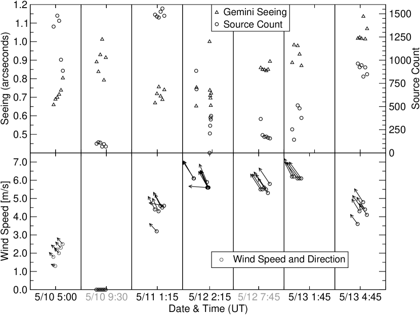
Figure 1: Forty-three images were acquired in two fields over four consecutive nights. The grey labels along the abscissa of the second and fifth viewing windows denote the second field. Image seeing and source counts are shown in the upper panel; wind speed and direction in the lower panel.

Frame	WDIR	WS	DATE	UT	AZ	SO	FWHM
36	317.0	1.8	050510	050106	-147.91	1436	0.718
37	293.0	1.3	050510	050210	-147.72	1652	0.748
38	308.0	2.2	050510	050313	-147.53	1543	0.753
39	318.0	2.0	050510	050416	-147.34	1493	0.788
40	318.0	2.3	050510	050519	-147.16	1112	0.818
41	319.0	2.5	050510	050622	-146.98	1004	0.886
43	333.0	4.4	050511	011041	146.25	1553	0.726
44	317.0	3.2	050511	011145	146.42	1535	0.788
45	335.0	4.3	050511	011247	146.60	1525	0.825
46	333.0	4.6	050511	011350	146.77	1582	0.766
47	331.0	4.5	050511	011452	146.95	1613	0.748
48	281.0	4.6	050511	011555	147.13	1542	0.809
52	330.0	6.1	050512	011507	147.70	1003	0.710
53	327.0	6.1	050512	011610	147.89	823	0.840
54	337.0	5.9	050512	020037	158.22	200	1.101
55	274.0	5.6	050512	020140	158.52	390	0.830
56	336.0	5.6	050512	020242	158.82	466	0.784
57	330.0	5.6	050512	020345	159.12	546	0.772
58	336.0	5.6	050512	020448	159.43	527	0.726
59	336.0	5.6	050512	020550	159.73	562	0.802
74b	333.0	6.2	050513	013053	151.69	430	0.993
75	332.0	6.2	050513	013155	151.92	329	1.088
77	323.0	6.1	050513	013401	152.41	665	1.080
78	323.0	6.1	050513	013505	152.65	636	1.029
79	324.0	6.1	050513	013607	152.90	542	0.965
87b	323.0	3.6	050513	044632	211.57	1074	1.136
88b	328.0	4.3	050513	044735	211.77	1039	1.165
89	324.0	4.5	050513	044837	211.96	1058	1.140
90	327.0	4.8	050513	044940	212.16	947	1.324
91	326.0	4.4	050513	045043	212.35	1037	1.145
92	326.0	4.1	050513	045146	212.54	970	1.242

Table 1: Header data from 31 Gemini GMOS images on field 1 (13^h40^m40^s $-$53°41′20″). The first 6 columns are extracted directly from the image headers; the last two columns are computed values. The headings from left to right refer to: (Abbreviated) frame number, wind direction (degrees), wind speed (m/s), date (yrmodd), universal time, telescope azimuth (degrees), source count and full width at half maximum (arcsec) defined as the median FWHM of the source objects in the preceding column. All angles are in degrees, North through East.

The lower plot in Figure 1 depicts the ground-wind speed and direction extracted from the image headers. Ground-wind speeds and direction were roughly constant, consistent with typical site conditions. The combined effects of low intrinsic source count, limited number of exposures and extensive cloud cover make the images from the second and fifth viewing windows difficult to analyze, hence they are excluded from subsequent discussion. A summary of header information from the remaining frames is contained in Table 1.

3 Analysis

Galactic stars are unresolved and the photons they emit are relatively unaffected by intervening dark matter, hence are excellent zero-ellipticity calibration objects. However, the atmosphere, instrument and shot noise all introduce spurious ellipticity which must be removed to recover the lensing signal. The success of a procedure in removing spurious ellipticity is directly tested by applying it to stars, whose PSF one knows a priori to be round: we therefore limit our study to stellar objects.

Considerable variation in ellipticity definition is found in the literature. Here we adopt the definition

$$\epsilon=\frac{1-\beta^{2}}{1+\beta^{2}},$$ (1)

in which $\beta$ is the ratio of the minor to major axes of the fitted ellipse. From this quantity one can construct the two independent ellipticity components $\epsilon_{1}$ and $\epsilon_{2}$

$$\epsilon_{1}= \epsilon\cos(2\phi)$$ (2)

$$\epsilon_{2}= \epsilon\sin(2\phi),$$ (3)

where $\phi$ is the angle between major axis of the ellipse and the x-axis of the detector. Systematic effects appear as correlations in ellipticity vectors across the image. To assess quanitatively the efficacy of correction procedures for removing PSF effects we define

$$\epsilon_{RMS} = \frac{1}{N}\displaystyle\sum_{i}^{N}(\epsilon_{{1},i}^{2}+\epsilon_{{2},i}^{2})^{1/2}$$ (4)

$$\bar{\epsilon} = \frac{1}{N}\left[\left(\displaystyle\sum^{N}_{i}\epsilon_{{1},i}\right)^{2}+\left(\displaystyle\sum^{N}_{i}\epsilon_{{2},i}\right)^{2}\right]^{1/2}$$ (5)

$$= (\bar{\epsilon}_{1}^{2}+\bar{\epsilon}_{2}^{2})^{1/2}.$$

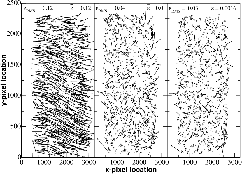
Figure 2: Raw ellipticities of 811 stars from frame 36 (left) and after vector subtraction of the average $\epsilon_{1}$ and $\epsilon_{2}$ ellipticities (middle). From its initial value of 0.12, $\epsilon_{RMS}$ is reduced to 0.03 after processing through the lensing pipeline (right). More significantly, $\bar{\epsilon}$ is reduced from 0.12 (left) to 0.0016 (right). Note that though (by construction) $\bar{\epsilon}$ in the middle plot is zero, correlations nonetheless persist among the objects, especially near the edges.

The first quantity $\epsilon_{RMS}$ is the root-mean-square ellipticity magnitude, while $\bar{\epsilon}$ is the average ellipticity. The sums in these equations are over all 811 stars. Both quantities vanish in the round star limit; the latter likewise vanishes if the ellipticity vectors are randomly oriented.

The three panels in Figure 2 show the ellipticities of 811 stars in frame 36 derived using steps 1-3 of the measurement procedure described in Section 3.3. (For reference, SExtractor identified a total of 1536 objects in the same frame.) The close agreement between $\epsilon_{RMS}$ and $\bar{\epsilon}$ in the leftmost panel reflects the high degree of correlation (presumably telescope tracking errors). A necessary next step is the removal of spurious ellipticity correlation, which otherwise mimics the weak lensing signal. A first order correction is to remove the common mode seen in that panel. The middle panel in Figure 2 is constructed in this manner, with $\epsilon^{{}^{\prime}}_{RMS}$ defined as

$$\epsilon^{{}^{\prime}}_{RMS}=\frac{1}{N}\displaystyle\sum_{i}^{N}((\epsilon_{{1},i}-\bar{\epsilon}_{1})^{2}+(\epsilon_{{2},i}-\bar{\epsilon}_{2})^{2})^{1/2}$$ (6)

replacing $\epsilon_{RMS}$ of Eqn. 4 and $\bar{\epsilon}_{1,2}$ defined as in Eqn. 5. The middle panel shows the effect of subtracting off the lowest order common mode. Though $\epsilon^{{}^{\prime}}_{RMS}$ has been reduced to 0.04, there remain persistent correlations, especially near the image corners. With this redefinition, $\bar{\epsilon}$ is identically zero. The rightmost panel in that same figure shows the ellipticities after processing the image through the entire pipeline. Here $\epsilon_{RMS}$ and $\bar{\epsilon}$ are reduced to 0.03 and 0.0016, respectively. More important, no obvious correlations persist. For this reason we make extensive use of the pipeline when discussing atmospheric residuals in Section 3.3.

Having emphasized the preeminent role that stars play in subsequent analyses and with some idea of the ellipticity magnitudes we now consider how their correlations depend on wind and seeing conditions.

3.1 Ellipticity Correlations with Wind

The next generation of weak lensing measurements will likely include high-fidelity simulations to disentangle systematic effects from the signal. A crucial component of these will be atmospheric simulations, which require, among other things, wind speed and direction as a function of height as their input. These data may or may not be readily available at many observing sites. Even if it does, it is still non-trivial to infer an effective wind direction and speed across the aperture. It therefore would be useful to extract wind information from the image itself as one is accustomed to do for seeing.

We see no wind information in the distribution of first moments of object intensities (seeing). However, it can be extracted by considering the second moments (ellipticities). The dominant ellipticity trend observed in the leftmost panel in Fig. 2 could well be attributed to the effects of wind transport across the aperture, but may also contain non-atmospheric components such as wind-shake of the telescope or guiding / tracking errors. We therefore cannot assume a priori that the dominant ellipticity trend is solely due to the wind.

To eliminate competing phenomena as the origin of the dominant ellipticity we perform pairwise vector subtraction of the raw ellipticity components of stars across the image, with the ellipticity components $e_{a}$ and $e_{b}$ derived from the shape parameter $\epsilon$ and position angle $\theta$ in the following manner

$$\epsilon= 1-{{e_{a}}\over{e_{b}}}$$ (7)

$$\tan{\theta}= {{e_{b}}\over{e_{a}}}.$$ (8)

As defined above, $e_{a}$ and $e_{b}$ are the lengths of the major- and minor axes of the ellipse, respectively. It follows that $\epsilon_{x}=\cos\theta$ and $\epsilon_{y}=\sin\theta$ are the ellipticity projections onto the x- and y-axes of the detector, respectively. The ellipticity residual is then defined as

$$\epsilon_{res}=((\epsilon_{{x},i}-\epsilon_{{x},j})^{2}+(\epsilon_{{y},i}-\epsilon_{{y},j})^{2})^{1/2}.$$ (9)

In constructing this latter quantity we arrive at a distribution of ellipticity residuals from which the common-mode ellipticity has been removed. The ellipticity residuals can be projected onto the rows and columns of the detector (as in Eq. 9), along the RA and DEC coordinate system, or along any other set of axes. (For an alt-az mount telescope like Gemini South a camera rotator is used to hold the instrument at a fixed position angle. For these data the position angle was such that the axes were aligned with RA and DEC.) In Fig. 3, we plot the magnitude of one of these components as a function of position angle. A position angle of 0° corresponds to a basis in which the x-axis corresponds to the RA direction, and the y-axis with the DEC direction. Any positive rotation is then counter-clockwise through the East. While the total magnitude of the ellipticity is a rotational invariant, the magnitude of the projected values are not. Fig. 3 plots the projection along the vertical axis; by construction the x-axis values are offset in phase by 90 degrees.

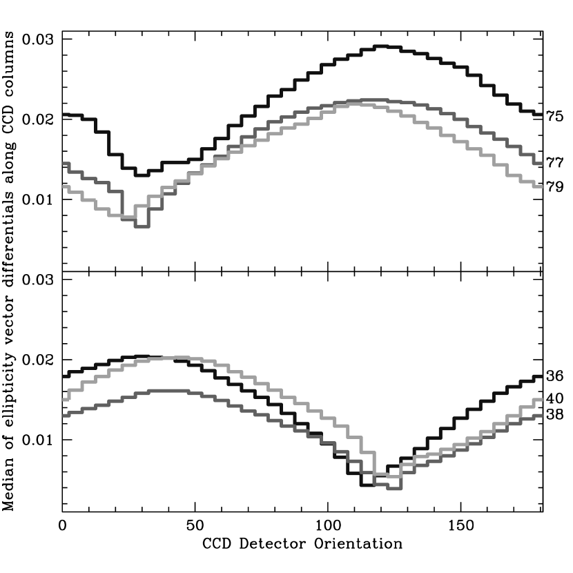
Figure 3: Median value of the $\epsilon_{y}$ ellipticity residuals (see Eq. 9) of the pair-wise combination of N = 150 stellar objects per frame (for a total of N(N-1) permutations), as a function of orientation angle of the CCD detector. (The x-axis curve (not shown) would appear identical, but shifted by 90 degrees.) The frame numbers are indicated on the right. The telescope was pointed approximately perpendicular to the ground wind direction in the bottom set of three curves, and along the wind direction in the top three. For each of the frames a preferred position angle exists for which the projected residuals are smallest along the y-axis (and consequently largest along the x-axis). This position angle can be interpreted as the direction for which the wind induces the longest correlation length, and therefore smallest residuals. The median stellar separation is 163$\arcsec$, with 25% of the pairs having separations less than 105$\arcsec$.

The curve for each frame (as indicated on the right side of the plot) has a distinctive minimum. Even though only a selected few frames are shown, all image data exhibit this behavior, albeit with lower significance for poorer seeing. Because the ellipticity residuals are at a minimum at a particular rotation, we can interpret this position angle as the direction in which the residuals are most correlated: a longer correlation length lowers the median ellipticity value as the PSFs are more similar along that direction. This stretching of the correlation length in a particular direction we believe is due to the more or less constant wind directions of the dominant wind layers (ground-layer and 200 mb jet-stream layer) across the telescope aperture. In essence, this transport of the air across the telescope ensures that otherwise uncorrelated regions of the detector see the same atmosphere, resulting in more similar PSFs along this effective wind direction.

During the observations the ground layer wind direction varied from 300 to 330 degrees (Fig. 1), with wind speeds of up to 6 m/s. The jet-stream layer was blowing due East with wind-speeds of about 30 m/s. If we assume that the wind directions are constant, then the only orientation variable left is the relative positioning of the telescope with respect to these winds.

Figure 4 summarizes the minima for all our image frames. It is clear that the data fall in two groups: one for which the telescope was pointed along the ground-wind direction (azimuth $\sim$150°, down triangles), and one pointed almost perpendicular to the ground-wind (azimuth $\sim 215\arcdeg$, up triangles). We find that that these minima are consistent over multiple days, ultimately reflecting similar observation and wind directions. The grey triangles all reflect observations of the same field taken about 2 hours before the meridian, and the black triangles 2 hours after the meridian. However, given the scatter in the data, we cannot uniquely identify these minima with a particular wind layer.

We furthermore note that for each frame the minima, even after taking out the bulk ellipticities through the pairwise subtractions, correlate with the direction of the bulk ellipticity (as given by the median ellipticity vector). The minima are found to be almost perfectly at right angles with the direction of largest ellipticity, and therefore closely align with the ellipticity minor axis. So, for these particular Gemini observations it is clear that most (if not all) of the bulk ellipticity observed in the frames is induced by the wind.

Given the predominant wind direction at Cerro Pachon and other sites, ellipticity residuals induced by the dominant wind layers are likely to persist over time. If an observing strategy involved viewing a part of the sky at similar hour-angles and telescope orientations, the result will be a persistent residual that will not diminish by averaging more images.

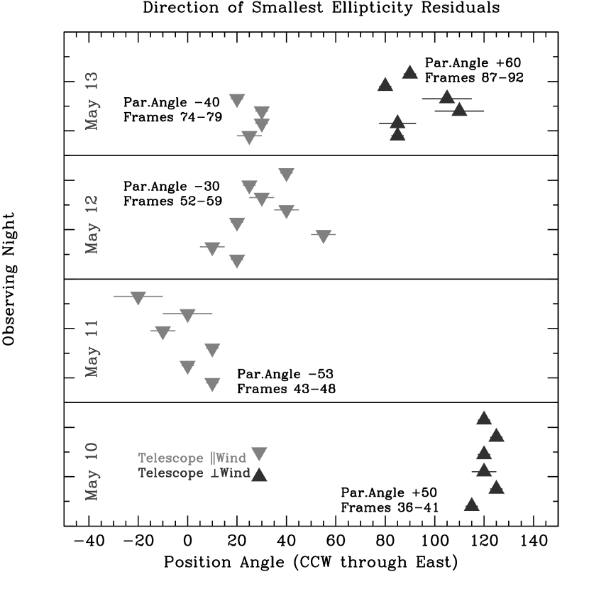
Figure 4: Direction of smallest ellipticity residuals. The up (black) triangles represent frames with the telescope pointing roughly perpendicular to the ground-wind; the down (grey) triangles where the telescope is pointing along the ground-wind. The telescope elevation is about 60 degrees above the horizon in all cases. The position angle has been plotted from -40 to 140 degrees for display purposes. The horizontal lines are indicative of measurement uncertainty.

3.2 Ellipticity Correlations with seeing

In this section we describe how the atmosphere affects the ability to characterize a PSF at a particular location on the detector, where intrinsically round stellar objects can acquire an ellipticity for reasons set forth in Section 1. Obviously, the better we can measure this unwanted ellipticity component the better we can correct for it.

The ability to interpolate over the image depends, in part, on the stellar density and atmospheric coherence. Under perfect seeing (and telescope) conditions a stellar wavefront is coherent and the PSF is known everywhere. Under finite seeing conditions the coherence distance is also finite. Coherence distances less than 1$\arcmin$ - the approximate separation of high-altitude galactic stars - would imply that there are locations in the image where the PSF is substantially unknown. This could impact weak lensing analyses, which relies on stellar objects to predict the PSF of galaxies. For this reason one would like to first establish the coherence distance as a function of seeing.

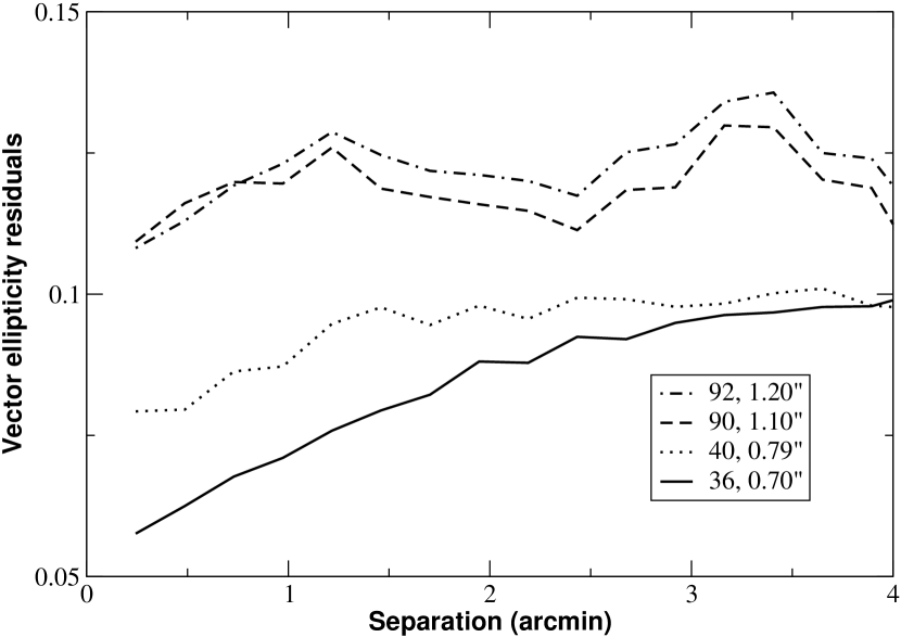
Figure 5: (left) Vector ellipticity residuals constructed from the 400 brightest stars of four images spanning a range of seeing conditions. The residuals were placed into 27 bins separated by $\sim$ 0.25$\arcmin$ out to a maximum separation of $\sim$ 6.5$\arcmin$, though statistics limit the useful range to below 4$\arcmin$. From each bin the median residual was extracted.

Figure 5 shows the vector ellipticity residuals of the 400 brightest stars as a function of separation for four frames spanning the range of seeing conditions in Table 1. Residuals are again constructed for each frame and placed into bins separated by $\sim$ 0.25$\arcmin$. The median residual was extracted and plotted. For good seeing the residuals are small for small separations. These residuals grow with increasing separation, reflecting atmospheric decoherence on these scales. This trend becomes less pronounced as the seeing gets worse. By the time the seeing is $\geq 1\arcsec$ the atmospheric is largely decoherent at all separations.

This analysis addresses the PSF behavior at stellar locations and demonstrates that under good seeing conditions the atmosphere exhibits some degree of coherence for small separations. To explore more quantitatively the useful limit of seeing we turn to the issue of the PSF behavior at an arbitrary location within the image. We choose two sets of stellar objects: fiducial and fixed. In what follows the PSFs of fiducial objects are measured and corrections are applied at the location of the fixed set. The density of the fiducial set is varied by selecting progressively fewer stars. It should be noted that this selection is not completely random: we always include the brightest objects (i.e., the density is lowered by removing the faintest stars first). This ensures that we are using the brightest and easiest to measure stars, mimicking the lensing pipeline methodology. This method also minimizes the impact of photon shot noise limitations to the ellipticity (see § 3.2.1). Using these fiducial stars we predict the PSFs of the other fixed set of stellar objects by calculating the (distance) weighted mean PSF derived from the fiducial set.

We use a fixed set of 150 stellar PSF positions randomly distributed across the chip. For each of these we calculate the vector ellipticity difference between the distance weighted mean PSF, calculated using a varying set of fiducial stars, and the actual PSF at these 150 positions. The y-axis of Fig. 6 is the median value ellipticity residual for the fixed set of 150 stars. The number of fiducial stars comprising the interpolation grid are varied from about 400 down to about 5, corresponding to a spatial density range of $\sim 14$ down to 0.2 stars per square arc minute (given our detector surface area of 29.2 square arcminutes).

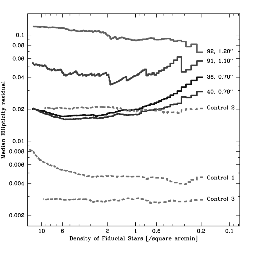
Figure 6: PSF interpolation as function of decreasing fiducial star spatial densityfor four selected images of the same field. The frame number and corresponding median seeing are shown. The control curves (marked 1 through 3) are based on artificial images containing round stars (0.7 $\arcsec$ seeing) selected from a brightness distribution of frame 36 (1), 20^th magnitude stars only (2), and 15^th magnitude stars only (3). Instances of good seeing ($<0.8\arcsec$) allow for excellent interpolation of the PSF down to densities of a few per square arc minute. The interpolation is limited by photon shot noise induced ellipticity, as illustrated by the dashed control 2 histogram. The upturn toward high spatial densities as seen in frames 36, 40, and control 1 is due to the progressive inclusion of fainter PSF objects in order to attain the required spatial density.

In Fig. 6 we plot the results for frames 36, 40, 91, and 92, whose variables span the range of observing conditions (cf. Table 1). The curve based on frame 36 represents the best observing conditions ($\sim 0.7\arcsec$ seeing), and will be discussed first. This curve is flat across spatial densities between 10 down to 2 stars / $\square\arcmin$, only to turn upward at higher and lower spatial densities. The upturn with decreasing spatial density is due to the gradual onset of spatial decorrelation between the PSFs due to the atmosphere. With separations of more than a few arc minutes the simple weighted interpolation invoked here poorly estimates PSF shapes. The upturn in the left part of the curve, on the other hand, is due to probable contamination by non-stellar objects (and their large intrinsic ellipticities) of the interpolation grid, as well as ellipticity measurement limitations of faint stars due to shot noise. We come back to this issue shortly.

Ignoring this high spatial density upturn, it is clear that with an interpolation grid of at least 1 star / $\square\arcmin$ residuals are minimized within this type of interpolation scheme. As the observation conditions worsen (as they do through frames 40, 91, and 92) ellipticity residuals rise regardless of PSF surface density, reproducing the trend seen in Fig. 5. For the (seemingly) pathological cases of frames 91 and 92, for which the PSF correlation length is essentially zero, we do not see an increase in the residuals with decreasing PSF surface density. Instead, we see a decrease due to the fact that in the lowest spatial density bins we only consider the brightest stars in the frame, which happen to be the ones with the smallest measurement errors. The spatial PSF decorrelation in these frames is such that it does not matter what PSF we use for our model.

3.2.1 Shot Noise contributions

To address how well this interpolation scheme performs, artificial sky images were created using a realistic observing and instrumentation setup. We use SkyMaker software to create three sets of images. The first (labeled “control 1” in Fig. 6) uses the brightness distribution found in frame 36. The other two images contained only stars of 20^th and 15^th magnitude (control 2 and 3 respectively). All stars are generated with a FWHM of 0.7 $\arcsec$ but no optical distortions are applied, hence the PSFs are perfectly round. Consequently, the sole source of ellipticity is photon number statistics, i.e., shot noise. Furthermore, as we have perfect PSF correlation across the chip, there should not be any trend with decreasing spatial PSF density. This is indeed what is seen in both controls 2 and 3 and the offset between these histograms is exactly what is expected from shot noise calculations. The fact that control 1 slopes upwards is due to the inclusion of progressively fainter stars as one goes up in spatial density (the faintest stars in control 1 are 19^th magnitude), which increases the shot-noise contribution.

Based on these control curves we can conclude the following. With ellipticity residuals on order of 0.02 (frame 36), we are within a factor of a few of the shot noise limit for $\sim$ 19^th magnitude stars, with the difference attributed to atmospheric turbulence. Second, for stellar surface densities of less than about $1/\square\arcmin$ this interpolation scheme is less successful. However, the roll-off is gradual, both in terms of PSF surface density and seeing conditions.

3.3 Full lensing analysis

Ellipticity correlations as formulated above are a powerful measure of coherence and PSF behavior, but are not expressed a form that is readily compared with a cosmological lensing signal. Further, more precise correction procedures are available than that applied above. We have chosen the Bernstein and Jarvis weak lensing analysis software (Bernstein & Jarvis, 2002) to correct stellar shapes for systematic effects. Much of the shape correction procedure is similar to that described in (Jarvis et al., 2003). However, not all elements of a pipeline expressly designed to measure galaxy shapes apply here, where we restrict our attention to stellar objects. Those that do apply are described briefly below.

1. Object Identification. All our analyses adopt SExtractor as their starting points. Aperture magnitudes and the zero-point magnitude suggested for GMOS are adequate for our purposes. Only well isolated stars having no associated error flags are selected.

2. Shape measurement. Ellipticities measured by SExtractor serve as initial estimates for more precise shape measurements based on second moments weighted by elliptical Gaussians.

3. Star Identification. Stars are discriminated from galaxies on the basis of size-magnitude considerations. To minimize the shot-noise contribution and further reduce contamination we selected the $N$ brightest candidates.

4. Convolution. A fiducial subset of these stars is chosen for rounding. The kernel required to round this subset is then interpolated to all other image locations. No correction is made for PSF dilution as described in (Jarvis et al., 2003).

5. Shape Remeasurement. With all stellar objects either directly or indirectly rounded via interpolation the shapes are remeasured. We do not correct for centroid bias, nor do we combine shape measurements.

A similar but distinct analysis has been carried out with data from the Subaru telescope on a single atmospheric realization (Wittman, 2005). There it was found that atmosphere-induced residuals are a factor of $\sim$ 20 or so below the the target signal level. Here we extend that study to a range of atmospheric conditions. The upper panel in Figure 7 shows the two-point correlation $\psi$, defined as

$$\psi=(\epsilon_{1}\epsilon_{1}+\epsilon_{2}\epsilon_{2})/4$$ (10)

for various object lists processed through the pipeline. The solid line is the correlation function constructed from 512 uncorrected stars from Frame 36, resulting in a constant $\psi\sim 0.002$ line. The lack of features in this curve reflects the dominant ellipticity trend evident in the leftmost panel in Fig. 2. The dotted curve is constructed from a fiducial subset of 122 rounded stars from that same frame. The dashed curve is again the correlation function of the same 512 stars, but with the fiducial subset of 122 stars now used for rounding and interpolation. The dashed-dotted curve is the correlation function constructed from 339 simulated stars that comprise the “Control 1” group of Fig. 6. Recall that “Control 1” can be considered the same as frame 36 but without atmospheric distortions. The correlation functions generated in this manner are bounded from above by the raw ellipticities (black curve) and from below by photon shot noise (dash-dotted curve), as expected.

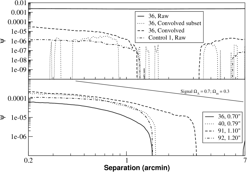
Figure 7: [Upper panel] The two point correlation function $\psi$ for various object lists processed through the pipeline. The solid, constant, line is the correlation function for 512 raw stellar objects from frame 36. That the curve is featureless and the amplitude large is a reflection of the sizable ellipticity correlation displayed in the leftmost panel in Fig. 2. The dotted curve is constructed from a subset of 122 rounded stellar objects ($\sim$ 25% of the total of 512). The erratic behavior observed in this curve arises from minimal statistics in numerous separation bins. The dashed curve is again the correlation function for the 512 stars, but now the 122 stellar objects have been used for rounding and interpolation. The dashed-dotted curve is the correlation function of 339 simulated stars that comprise the “Control 1” group from Fig. 6. [Lower panel] The two-point correlation functions for frames 36, 40, 91 and 92 constructed in manner similar to the dashed curve in the upper plot, but instead using 30 of the brightest stars as the fiducial subset. Only positive values of $\psi$ are shown. The solid line is the level of the expected signal for a cosmology with $\Omega_{\Lambda}$ = 0.7, $\Omega_{m}$ = 0.3 and z = 1 (Jain & Seljak, 1997).

The lower panel in Figure 7 was generated in an analogous manner to that used to produce the dashed curve in the upper plot, but is carried out for frames 36, 40, 91 and 92 using just 30 of the brightest stars in each frame as fiducial stars. The convolution was then applied to the remaining stars. The roll off exhibited by each of the curves for separations above a few arcseconds is understood in terms of the density of fiducial stars ($\sim$ 1/$\square\arcmin$ to match the typical density of high-latitude stars). For separations below a few arcseconds the correlations rise monotonically, reflecting the imperfect interpolation process between fiducial stars. However, even for the smallest separations this procedure results in an improvement on systematics shape 3-10 times over that in the raw images. Under all seeing conditions and for all separations the uncorrectable power $\psi$ is at worst a factor of five or so below that of the expected lensing signal (Jain & Seljak, 1997). For separations relevant to present surveys ($\sim$ 1$\arcmin$ or more) the systematic error arising from uncorrectable atmospheric power (for good seeing) is of comparable magnitude to the statistical error ($\sim$ 0.003) (Jarvis et al., 2006, Fig.1). The lack of an exact one-to-one correspondence between seeing and amplitude of the two-point correlation functions is attributed to fluctuations, as well as variations in the number of test stars in the four frames.

4 Conclusions

Many systematic effects will affect data from the next generation of weak lensing instruments. To understand the impact of the varying atmosphere we have acquired simultaneous image and atmospheric data from the Gemini South telescope. The exposure time of 15 s, site location and mirror diameter are matched to that of the proposed Large Synoptic Survey Telescope (Tyson et al., 2005).

We have studied the effects of atmospheric turbulence using three methods of increasing sophistication and demonstrate that with seeing conditions up to $\sim$ 0.7$\arcsec$ the PSF is coherent over appreciable angular scales. When seeing exceeds 1$\arcsec$, the atmosphere is largely decoherent over all angular scales. We find that these correlations are not isotropic. Rather, there is a preferred direction, which we find to be induced by persistent wind layers. Unless somehow corrected for, this correlation will persist even after image stacking. Using a simple interpolation technique and under good seeing conditions the PSF can be predicted to within a factor of a few of the theoretical (shot noise) limit. A complete weak lensing analysis demonstrates that for data taken under less than ideal circumstances atmospheric residuals can be reduced below that of the target cosmic shear signal. The presence of fiducial stars at a nominal density of $\sim$ 1/$\square\arcmin$ provides for sufficient sampling of the image plane to compensate for atmospheric decoherence. Under the best seeing conditions we confirm an earlier result (Wittman, 2005) and further note that the uncorrectable systematic errors are of the order of statistical errors associated with present lensing surveys. However, future surveys will measure many more shapes and the statistical errors will be correspondingly reduced. Thus, the present level of systematic error must also be lowered, especially in the non-linear regime. A priori, it is not obvious how one would commensurately lower the systematic error attributed to the atmosphere using the procedure outlined in this paper (since the errors are proportional to the fixed density of stellar objects used to make shape corrections). Fortunately, future surveys will revisit the same patch of sky multiple times and one can resort to shear-shear correlations computed from shear measured across frames (first discussed in Jarvis & Jain, 2004). If these frames are well separated temporally (e.g. $>$ 20 s) then the atmospheric noise is purely stochastic and will not add systematic power to shape measurements (see Jain et al., 2006, for a methodology that minimizes the information lost from not computing shear correlations within an image).

References

- Bartelmann & Schneider (2001) Bartelmann, M. & Schneider, P. 2001, Physics Reports, 340, 291
- Bernstein & Jarvis (2002) Bernstein, G. & Jarvis, M. 2002, AJ, 123, 583
- Fischer et al. (2000) Fischer, D. et al. 2000, AJ, 120, 1198
- Hook et al. (2006) Hook, I. et al. 2006, PASP, 116, 425
- Jain & Seljak (1997) Jain, B. & Seljak, U. 1997, AJ, 560
- Jain et al. (2006) Jain, B. et al. 2006, Journal of Cosmology and Astroparticle Physics, 1
- Jarvis & Jain (2004) Jarvis, M. & Jain, B. 2004, astro-ph/0412234
- Jarvis et al. (2003) Jarvis, M. et al. 2003, AJ, 125, 1014
- Jarvis et al. (2006) —. 2006, ApJ, 644, 71
- Mellier & van Waerbeke (2001) Mellier, Y. & van Waerbeke, L. 2001, in Where’s the Matter?, ed. M. Treyer & L. Tresse (Frontier Group)
- Tyson et al. (1990) Tyson, J. et al. 1990, ApJL, 349, 1
- Tyson et al. (2005) —. 2005, Bulletin of the AAS, 207
- Wittman (2005) Wittman, D. 2005, ApJL, 632, 5