Dynamical Evidence for Environmental Evolution of Intermediate Redshift Spiral Galaxies

Abstract

Combining resolved optical spectroscopy with panoramic HST imaging, we study the dynamical properties of spiral galaxies as a function of position across two intermediate redshift clusters, and we compare the cluster population to field galaxies in the same redshift range. By modelling the observed rotation curves, we derive maximal rotation velocities for 40 cluster spirals and 37 field spirals, yielding one of the largest matched samples of cluster and field spirals at intermediate redshift. We construct the Tully-Fisher relation in both $V$ and $K_{S}$ bands, and find that the cluster Tully-Fisher relation exhibits significantly higher scatter than the field relation, in both $V$ and $K_{S}$ bands. Under the assumption that this increased scatter is due to an interaction with the cluster environment, we examine several dynamical quantities (dynamical mass, mass-to-light ratio, and central mass density) as a function of cluster environment. We find that the central mass densities of star-forming spirals exhibit a sharp break near the cluster Virial radius, with spirals in the cluster outskirts exhibiting significantly lower densities. We argue that the lower-density spirals in the cluster outskirts, combined with the high scatter in both $K_{S}$- and $V$-band TF relations, demonstrate that cluster spirals are kinematically disturbed by their environment, even as far as $2R_{VIR}$ from the cluster center. We propose that such disturbances may be due to a combination of galaxy merging and harassment.

1. INTRODUCTION

The observed tight correlation between the rotation velocities of spiral galaxies and their total luminosities, first noted by Tully & Fisher (1977), has proven invaluable in helping to pin down the extragalactic distance scale in the local universe (e.g. Tully & Pierce, 2000). Since then, many authors have attempted to leverage the so-called Tully Fisher relation to study the evolution of spiral galaxies as a function of redshift, generally interpreting any deviation from the local Tully Fisher (TF) relation as an evolution in luminosity.

These studies have yielded mixed results, however, with conflicting estimates of the rate of B-band evolution as a function of redshift (Bamford et al., 2006; Böhm et al., 2004; Milvang-Jensen et al., 2003; Vogt et al., 1996). Recently, several authors have documented many of the systematic errors that make comparisons between studies very difficult (Metevier et al., 2006; Nakamura et al., 2006). Indeed, Nakamura et al. (2006) argue that the most certain method of using the TF as a measure of evolution is to construct a large matched sample of galaxies, consisting of nearly equal numbers of cluster and field galaxies all measured in the same way.

In a similar manner, large matched samples such as those presented by Nakamura et al. (2006) and Bamford et al. (2005) can also be effectively used to measure a different sort of spiral galaxy evolution: that caused by infall into a galaxy cluster. By carefully selecting galaxies across a wide range of environments, in and out of clusters, we can gain a better understanding of the changes in star formation and kinematics that a spiral may undergo as it falls into a cluster potential.

In this paper, we attempt to construct such a sample out of a large survey we are performing of two massive galaxy clusters at intermediate redshift: Cl 0024+17 (hereafter Cl 0024) at $z=0.39$ and MS 0451-03 (hereafter MS 0451) at $z=0.54$, which were selected to be complementary in their global properties, as part of a larger project to understand the role of the cluster environment in galaxy evolution. We make use of high quality spiral rotation curves determined from Keck spectroscopy to measure the Tully Fisher relation. The sample is large enough to allow a first investigation of the scatter of the relation as a function of cluster-centric radius. We also study a control sample of field galaxies in a range of redshifts centered about the cluster redshifts, in order to asses differences between field and cluster spirals. Our sample of 40 cluster galaxies is the largest yet reported with an associated field sample (37 galaxies), and provides a powerful means to examine the effect of the cluster environment on infalling star-forming spirals.

In order to disentangle environmental processes affecting the dynamics of infalling spirals and those affecting their stellar populations, we contrast the trends in the TF relation with those observed for integrated $V-K_{S}$ colors and disk mass density. The latter quantity is constructed from rotation curves and HST scale lengths, and is predicted to be sensitive to the strength of the ‘harassment’ process (Moore et al., 1999).

A plan of the paper follows. In § 2, we describe our cluster survey and sample selection, and then detail our procedure for deriving maximal rotation velocities in § 3. In § 4, we present our results on the cluster and field Tully Fisher relation, with an examination of other dynamical quantities in § 5. The Tully Fisher relation in Cl 0024 has also been studied by Metevier et al. (2006), and in § 4 we also directly compare rotation measurements for several galaxies in common between studies. In § 6 we discuss these results in light of proposed physical mechanisms acting in the cluster environment. In this paper, we adopt a cosmology with $\Omega_{m}=0.3$, $\Omega_{\Lambda}=0.7$, and $H_{0}=70\textrm{km s}^{-1}\textrm{Mpc}^{-1}$.

2. OBSERVATIONS

In this study, we leverage a large imaging and spectroscopic survey of two massive intermediate redshift clusters: Cl 0024 at $z=0.39$ and MS 0451 at $z=0.54$, yielding high quality spectra of both field and cluster spirals, suitable for extracting rotation curves. In the following, we describe our photometric and spectroscopic observations, data reduction, and sample selection.

2.1. Imaging

We make use of HST imaging of Cl 0024 and MS 0451 from the comprehensive wide-field survey described in Treu et al. (2003) and Smith et al. (2006, in preparation). In Cl 0024, HST coverage consists of a sparsely-sampled mosaic of 39 WFPC2 images taken in the F814W filter ($\sim I$ band), providing coverage to a projected radius $>5$ Mpc. MS 0451 observations were taken with the ACS, also in F814W, and provide contiguous coverage within a 10Mpc$\times$10Mpc box centered on the cluster. Both sets of observations are complete to $F814W>25$.

For Cl 0024, Treu et al. (2003) reported reliable morphological classifications to $I=21.1$. The MS 0451 observations are proportionately deeper, and so reliable morphological classification is possible to the same rest frame absolute magnitude ($M_{V}=-19.5$). All galaxies brighter than this limit are classified visually following Treu et al. (2003).

We also use panoramic ground-based $K_{s}$-band imaging of both clusters, and J-band imaging of Cl 0024, with the WIRC camera (Wilson et al., 2003) on the Hale 200” Telescope. These data comprise a $3\times 3$ mosaic of pointings, spanning a contiguous area of $26^{\prime}\times 26^{\prime}$ centered on each cluster. Observations were made in 2004 November for MS 0451 and 2002 October for Cl 0024. The details of the observations and data reduction are described by Smith et al. (2005) and Smith et al. (2006, in prep.) for Cl 0024 and MS 0451, respectively. Point sources in the final reduced mosaics have a full width half maximum of 0.9” and 1.0” in Cl 0024 and MS 0451 respectively, and the $3-\sigma$ point source detection thresholds are $J=21.6$ and $K_{s}=19.7$ for Cl 0024 and $K_{s}=20.2$ for MS 0451.

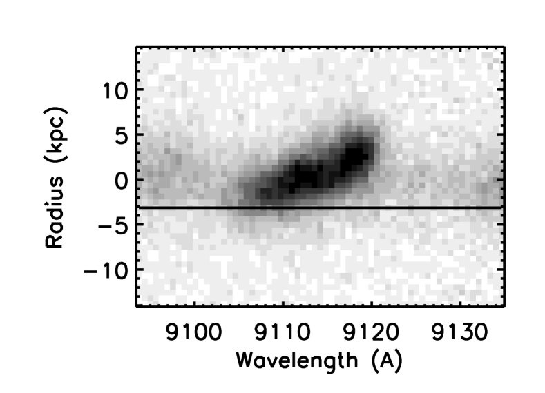
Figure 1.— Top: Postage stamp image of a 2D spectrum, centered on the observed wavelength of H$\alpha$ for the galaxy N57426, in the field of MS 0451. The solid line across the image indicates the spectral row that is plotted in the lower panel. Bottom: One spectral row from the 2D spectrum. The solid curve indicates the Gaussian fit to this row. The stellar continuum emission has been subtracted according to the method described in the text.

These near-infrared data are supplemented with wide-field ground-based optical imaging. We make use of BVRI-band imaging of Cl 0024 with the 3.6-m Canada-France-Hawaii Telescope using the CFH12k camera (Cuillandre et al., 2000), full details of which are available in Czoske et al. (2002) and Treu et al. (2003). MS 0451 was observed by Kodama et al. (2005) for the PISCES survey through the BRI-band filters using Suprime-Cam on the Subaru 8-m Telescope. Full details of these data are published by Kodama et al. (2005). The CFH12k data reach $3-\sigma$ depths of $B=27.8$, $V=26.9$, $R=26.6$ and $I=25.9$ in $\sim 0\farcs 9$ seeing, and the Suprime-Cam data reach $3-\sigma$ depths of $B=28.1$, $R=27.3$, $I=25.8$ in seeing ranging from $0\farcs 6$ to $1\arcsec$. The field of view of all of these optical data is well matched to the area surveyed by the near-infrared mosaics discussed above.

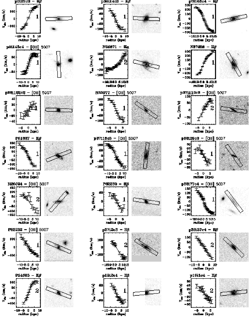
Figure 2.— Postage stamp images and rotation curves for cluster spirals, arranged in order of ascending projected radius, $R$, normalized by each cluster’s Virial radius $R_{VIR}$. HST images are $9\arcsec\arcsec$, in F814W. Observed rotation curves are plotted as error-barred points, solid lines represent the best-fit rotation curve model, and the quality code is displayed on the plot. Radii in kpc are measured along the semimajor axis. In case where more than one emission line yielded a rotation curve, we plot the best one. On the postage stamp images, the position of the $1\arcsec\times 8\arcsec$ slit is indicated by the solid black box. Some slits are not aligned with the galaxy major axis. At the redshift of the clusters, the spectroscopic seeing of $0\farcs 8$ is equivalent to $\sim 4.5kpc$.

Fig. 2. — (Cont.)

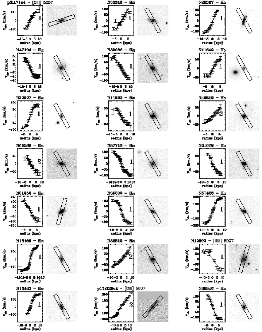
Figure 3.— Postage stamp images and rotation curves for all field spirals, arranged in ascending redshift order.

Fig. 3. — Continued.

2.2. Spectroscopy

Observations with the DEIMOS spectrograph on Keck II from October 2001 to October 2005 secured spectra for over $500$ members of both Cl 0024 ($0.373<z<0.402$) and MS 0451 ($0.520<z<0.560$). Details are provided in Treu et al. (2003), Moran et al. (2005), and Moran et al. (2007, in prep). Briefly, we observe with $1\arcsec\times 8\arcsec$ slits, with a typical velocity resolution of 50 km s^-1. For each cluster, spectral setups were chosen to span rest frame wavelengths from $\sim 3500\mbox{\AA}$ to $\sim 6700\mbox{\AA}$, covering optical emission lines [OII],[OIII], H$\beta$, and, more rarely, H$\alpha$. Exposure times totaled 2.5hrs in Cl 0024 and 4hrs in MS 0451. In this spectroscopic survey, we have also obtained spectra for over 2500 field objects, with 700 having redshifts similar to the clusters ($0.3<z<0.65$).

DEIMOS data were reduced using the DEEP2 DEIMOS data reduction pipeline (Davis et al., 2003), which produce sky-subtracted, wavelength-calibrated two-dimensional spectra, suitable for identifying and extracting extended optical emission lines. Redshifts for all galaxies were verified by eye.

2.3. Sample Selection

Our current sample is drawn from the set of surveyed galaxies with both HST imaging and available spectra. From the HST imaging, we select candidate galaxies that are morphologically classified as spirals (T-types 3, 4, or 5). For ease of comparing cluster spirals to field, we construct a matched sample of field spirals, all with HST imaging from the Cl 0024 or MS 0451 mosaics, and selected to lie in a redshift range that brackets the two clusters, $0.3\leq z<0.65$.

In our spectroscopic survey, targets were selected randomly from an F814W-limited sample, to $F814W=22.5$ in the field of Cl 0024, and to $F814W=23.0$ in MS 0451. Here, we focus on a subset of these galaxies that have been observed with slits aligned along the galaxy major axis, in order to secure resolved spectra of spirals with extended emission lines. The Cl 0024 campaign primarily targeted known cluster spirals for spectroscopy along the major axis, but serendipitous alignments with the major axes of field galaxies allowed us to include some of these in our sample. In MS 0451, we observed most galaxies with aligned slits, and, as a result, our field sample of spirals is weighted toward galaxies in the field around MS 0451.

As our field sample is composed of objects in the same redshift range as the clusters, biases introduced by the magnitude-limited survey should affect both samples equally, except at the faint end of the luminosity function. This effect will be discussed further in § 4.

2.4. Source Extraction and Photometry

Photometry was measured using SExtractor version 2.2.2 (Bertin & Arnouts, 1996). For ground-based imaging, we use SExtractor in two-image mode with source detection performed on the ground-based I-band images. Source detection on the HST images was performed independently, and then matched to the ground-based catalog. For all imaging, we adopt magnitudes from the MAG_AUTO measurement of SExtractor. Cl 0024 $K_{S}$ images are not deep enough to detect all cluster spirals of interest; we therefore report $K_{S}$ magnitudes only for objects detected with $>3\sigma$ significance.

The kcorrect software v.4_1_2 (Blanton et al., 2003) was used to convert observed $K_{S}$ and F814W fluxes to absolute magnitudes, $M_{K_{S}}$ (hereafter $M_{K}$) and $M_{V}$, respectively. At the redshifts of the clusters, observed $I$-band corresponds closely to rest-frame $V$, and so the k–corrections are small ($<0.5mag$). In determining the k-corrections, we make use of all available ground-based photometry for each cluster field. This yields a better k–correction due to better sampling of the galaxy spectral energy distributions. For field objects at the low end of our redshift range, observed $R$-band is a closer match to rest-frame $V$ than observed $I$, and so for these objects we apply a k–correction to the $R$ magnitudes to determine $M_{V}$. Before determining the k–corrections, we correct for a Galactic extinction of E(B–V)=0.056 or E(B–V)=0.033, for Cl 0024 and MS 0451, respectively (Schlegel et al., 1998). All absolute magnitudes are expressed on the AB magnitude system.

3. Rotation Curve Analysis

In order to construct the Tully Fisher relations, and to study other kinematic properties of spirals (such as mass, density, or M/L), we seek to determine the maximum velocity of the rotation curve for each disk. Our process involves extracting the observed rotation curve from the spectrum and then creating artificial rotation curves for each galaxy, determining the best-fit maximum velocity by $\chi^{2}$ fitting against the extracted rotation curve. In order to do this is important to determine various parameters about the galaxy from photometric data including: the position angle of the slit with respect to the position angle of the major axis of the galaxy, the scale length of the galaxy and the seeing when the galaxy was observed. Along each step, we filter out the galaxies with weak spectral lines or those which, for reasons of inclination, etc. would not be possible to fit using our model. We further divide the remaining fits into two subsamples, those with secure rotation velocities ($Q=1$), and those where the velocity is less certain but probably correct ($Q=2$). We largely follow the procedure of Böhm et al. (2004), though several other authors have followed similar procedures (e.g. Metevier et al., 2006; Nakamura et al., 2006; Bamford et al., 2005; Vogt et al., 1996). We have made several modifications to the procedure, detailed below.

3.1. Extraction of Rotation Curves

From each complete 2D spectrum, we extract postage stamps about the position of every emission line present, using the known redshift of each object to identify lines. In the top panel of Figure 1, we display an example postage stamp centered on H$\alpha$ for the galaxy N57426, a $z=0.39$ field galaxy in the vicinity of MS 0451. As the observed center of H$\alpha$ emission clearly varies across the spatial dimension of the spectrum, the rotation in this galaxy is already apparent. In order to determine the observed rotation curve, we fit a Gaussian function or double Gaussian (in the case of [OII]) to each row along the spectral direction, as demonstrated in the lower panel of Figure 1. For the double Gaussian, we assumed a fixed separation and that the FWHM of each Gaussian component was the same, but allowed the amplitudes to differ independently.

We bin spectral rows together in the spatial dimension, as necessary, to meet a signal to noise (S/N) requirement of $\sim 5(\mbox{\AA}^{-1})$ per bin. This re-binning allows us to sum up regions of the emission line that are too faint to fit individually, essentially trading spatial resolution, which is less important near the outer flat regions of a rotation curve, for a more reliable velocity measurement. When rows are binned, the x position (i.e. radius) of the resulting velocity point is calculated by taking a S/N weighted mean of the x positions of all the constituent spectral rows.

Each of these binned fits were checked by hand to ensure that they were meaningful. All extracted rotation curves for our complete sample are displayed in Figures 2 and 3.

We found that the fit worked best when we subtracted off the continuum to all the rows before fitting. We measured the continuum on the spectrum for each spectral line separately by summing together about 50 spectral columns on either side of the emission line’s center. By extracting and continuum subtracting over small postage stamps, we avoid any issues that might be caused by spatial distortion in the spectrum.

3.2. Surface Photometry

From our HST imaging, we extract a $9\arcsec\times 9\arcsec$ postage stamp image of each galaxy in our sample, with the galaxy centered (See Figures 2 and 3.). We then use the GALFIT software (Peng et al., 2002) to fit the galaxy photometry to a Sersic profile. This fit yields estimates of the galaxy position angle on the sky, axis ratio, and scale length. These parameters are necessary to determine the maximum velocity of the galaxy in the following step. While we experimented with fitting to an exponential disk plus bulge component, we find that the scale length as derived from the Sersic profile fit yields the best estimate of the rotation curve turn-over scale length, as described below.

In local Tully-Fisher studies, internal extinction of spiral galaxies has been found to depend on the galaxy’s inclination to the line of sight (Tully & Fouque, 1985; Tully et al., 1998; Verheijen, 2001). Galaxies viewed close to edge-on have a larger fraction of their luminosity extinguished by dust than the same galaxy would have if viewed face on. We correct for this effect by adopting the particularly simple form of the correction introduced by Tully et al. (1998):

$$A_{\lambda}=-\gamma_{\lambda}\log\left(\frac{a}{b}\right)$$ (1)

where $a/b$ is the axis ratio of the galaxy. This formula corrects toward the face-on case, but does not correct for additional extinction in a face on galaxy. We choose not to apply any additional correction for the internal extinction of a face-on galaxy.

Following Tully et al. (1998), we determine $\gamma$ in each band by minimizing the scatter in the rest-frame color magnitude relations $B-K_{S}$ vs. $M_{K}$ and $V-K_{S}$ vs. $M_{K}$, using the entire cluster plus field sample together. Since the luminosity function of cluster spirals may not be uniform across all studied environments, we ignore any luminosity dependence of the $\gamma$ correction, in order to avoid ‘fitting away’ real deviations that may be due to the cluster environment. We find $\gamma_{B}=1.37$, $\gamma_{V}=1.12$, and $\gamma_{K}=0.15\times\gamma_{B}=0.206$. These values are consistent with the range specified in, e.g., Tully et al. (1998) and Verheijen (2001).

3.3. Model Fitting

In order to determine the peak rotation velocity of a galaxy, we used the parameters obtained from GALFIT to construct an estimated velocity field for some maximum velocity. We adopt a standard rotation curve function of the form

$$V(r)=\frac{V_{MAX}r}{(r^{a}+r_{s}^{a})^{1/a}}$$ (2)

where $r_{s}$ is the Sersic profile scale length as determined by GALFIT and $a=5$, following Böhm et al. (2004). For two galaxies in our sample, p1i97c4 and N46608, $r_{S}$ from GALFIT appeared to be an overestimate of the rotation curve scale length, and so we manually adjusted it to achieve a better fit. From the intrinsic rotation curve specified above, we construct a 2D velocity field by populating a grid of line-of-sight velocities, under the following formula:

$$V_{\textrm{obs}}=V(r)\cdot cos(\phi)\cdot sin(i)$$ (3)

where $\phi$ is the azimuth in the plane of the disk and $i$ is the inclination, with $i=90^{\circ}$ defined to be edge-on to the line of sight.

Table 1Summary of sample selection.

	Cl 0024	MS 0451	Field	Total
	$0.37<z<0.41$	$0.52<z<0.56$	$0.3<z<0.65$
a. Spirals in the specified redshift range with HST imaging and DEIMOS spectra	103	130	194	427
b. Those with extended emission lines and aligned slits	92	103	62	257
c. Significant spatial extent, with a measured velocity gradient	42	26	47	115
d. After removing very face-on galaxies and other mis-aligned slits	28	16	38	82
e. Velocity uncertainty small enough	24	16	37	77
f. Q=1 rotation curve	17	11	30	58

We then convolve this velocity field with a point spread function (PSF) with FWHM equal to the seeing. For our data, we used a fixed seeing of $0.8\arcsec$, equal to the median seeing of our observations. We adopt this fixed seeing correction because of the relative insensitivity of the results to small variations in seeing; we find that our uncertainty in the seeing correction affects the final $V_{MAX}$ by $<1\%$, which is insignificant compared to errors due to inclination or position angle.

Then, comparing the slit PA of our observation to the GALFIT estimate of the galaxy major axis angle, we place a mock $1\arcsec$-wide slit across the model velocity field, at an angle reflecting the alignment between the real slit and the galaxy major axis. Finally, at each position along the length of the slit, we averaged the pixels across the slit width to determine an observed velocity. We use a $\chi^{2}$ minimization technique to vary the maximum velocity in the model to match our observed rotation curves.

For each observed spectrum, we estimate the position of the galaxy’s spatial center by fitting a Gaussian function to the spatial profile of the 2D absorption spectrum, integrated along the spectral dimension in two bands bracketing the emission line of interest. An initial estimate of the velocity center is calculated from the previously-determined redshift of each galaxy. Both the spatial center and velocity center are left to be free parameters in the $\chi^{2}$ minimization. However, in no case does the best-fit spatial center of a $Q=1$ rotation curve differ by more than two pixels ($\sim 1.5$ kpc physical) from the calculated position, with typical offsets of much less than one pixel.

We first fit the rotation curve using fixed values for the PA and inclination, $i$. In order to determine the error values on our fits, we factor in the error from the fit as well as computing a PA error and inclination error for the model by running it at $\pm 10^{\circ}$ for each parameter. Especially for galaxies that present a somewhat face-on profile, it is important to account for this uncertainty due to PA and inclination errors, as it can be large in some cases, and in fact causes us to discard several emission line galaxies from our sample. We choose to vary over $\pm 10^{\circ}$ because the formal errors in the photometric fit are small in comparison to the systematic uncertainty in measuring the PA and inclination from the inherently asymmetric light profile of a spiral galaxy.

3.4. Quality Control

We began with a sample of 257 candidate spiral galaxies, each with visible, spatially resolved emission lines. Out of this sample, we removed 142 galaxies because the rotation curve lacked enough spatial extent to detect a reliable turn-over, or else no significant velocity gradient was measured, in most cases because the galaxy is oriented nearly face-on. Additionally, we removed 33 galaxies because the spectroscopic slit was too misaligned, or because the galaxy appeared too face-on to estimate the direction of its major axis.

After fitting models to the rotation curves of our candidate spirals, and culling bad fits from our sample as described above, we remove five additional objects with highly uncertain velocities, $\Delta Log(2V_{MAX})>0.2$. Our final sample then consists of 37 field spirals and 40 cluster spirals (24 from Cl 0024). The observed rotation curves, model fits, and images of these galaxies are presented in postage stamp form in Figures 2 (cluster galaxies) and  3 (field galaxies).

We further divide this sample into two quality classes: $Q=1$ rotation curves have turnovers detected on both sides of the curve, with a model fit that accurately matches the turnover at each end. $Q=2$ curves, about 25$\%$ of the total, only show a turnover at one end, or show other signs of an uncertain fit to the model. We do not simply throw out all galaxies with signs of disturbed kinematics, but rather keep them in the $Q=2$ sample, as they are of considerable interest for our study of possible interactions with the cluster environment. However, the requirement that we identify a reasonably secure value of $V_{MAX}$ must necessarily exclude some number of spirals with highly disturbed rotation curves.

We summarize the sample selection process for both clusters and the field in Table 1. We note that we remove roughly equal fractions of galaxies from the cluster and field samples, at each step of the process. The two notable exceptions have ready explanations: In step b.), a larger fraction of field galaxies than cluster galaxies are removed due to misaligned slits, because we did not consistently observe field galaxies with aligned slits. Similarly, in step c), a low fraction of MS 0451 cluster galaxies exhibited large enough spatial extent in their rotation curves, due to an observed suppression or lack of star formation across this massive cluster (Moran et al. 2007, in prep). Basic data, as well as extinction-corrected magnitudes and velocities for all 77 objects of our main sample are listed in Table 3.

4. The Tully Fisher Relation

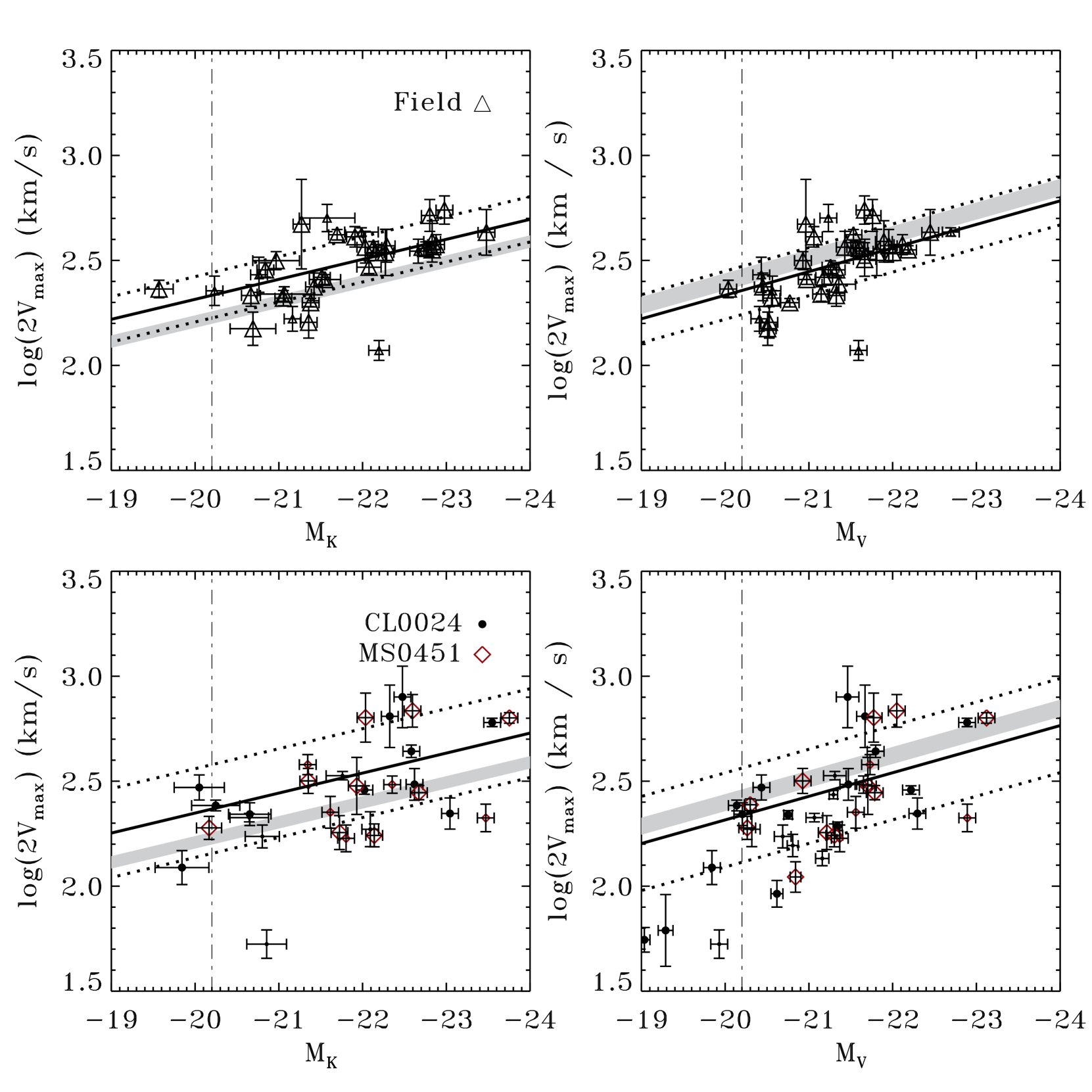
Figure 4.— V–band (right) and K–band (left) Tully-Fisher relations for cluster and field spirals. The field relation is plotted in the top two panels, and cluster galaxies are plotted on the bottom. Cl 0024 members are marked as black circles, while MS 0451 members are indicated by red diamonds. Shaded regions indicate the $1-\sigma$ scatter of the local Tully-Fisher relation, from Verheijen (2001). We adopt their R-band relation to compare to our V-band relation, neglecting any small correction to account for the different filters. In each panel, the thick solid line represents the inverse–fitted TF relation for those points (but fixing the slope to the local value), and the dotted lines represent the $1\sigma$ scatter about the mean. Dash-dotted line indicates where we apply a cut in magnitude for this calculation. Symbols are as indicated by the legend; small symbols indicate $Q=2$ rotation curves, and large symbols are $Q=1$.

In Figure 4, we plot the Tully Fisher relation for both cluster and field galaxies, in both rest frame $K_{S}$ and $V$ bands (expressed as absolute magnitudes $M_{K}$ and $M_{V}$, respectively). Shaded regions indicate the $\pm 1-\sigma$ scatter of the local TF from Verheijen (2001). Solid lines indicate the best fit TF zero point for each of our subsamples, with the slope fixed to the local values from Verheijen (2001), adopting their RC/FD sample, which includes only galaxies where a turnover in the rotation curve is seen. Dotted lines indicate the $1-\sigma$ RMS scatter of the relation about the mean. Zero points are calculated by finding the bi-weight mean of the residuals about the local TF. To minimize bias, zero point and scatter are calculated only from $Q=1$ rotation curves. We further impose an absolute magnitude cut of $M_{V}\leq-20.2$ and $M_{K}\leq-20.2$, to eliminate bias due to the differing magnitude distributions between the cluster and field samples.

For purposes of determining the intrinsic scatter in the TF relation for each of our samples, we also perform a least-squares fit to find the best-fit parameters of the TF relation, weighting each point by the measurement uncertainties in both $Log(2V_{MAX})$ and absolute magnitude. We follow other authors (e.g. Bamford et al., 2006; Metevier et al., 2006; Nakamura et al., 2006) and adopt $Log(2V_{MAX})$ as the dependent variable in the fit, such that

$$Log(2V_{MAX})=a+b*M_{V,K}$$ (4)

where we fit for intercept a and slope b. This is the so-called ‘inverse TF’, which is less sensitive to bias due to luminosity incompleteness (Willick, 1994; Schechter, 1980). For each TF relation, cluster and field, $V$ and $K_{S}$ bands, the intrinsic scatter is that portion of the measured scatter that cannot be explained by measurement error. We estimate the intrinsic scatter by considering the reduced $\chi^{2}$ statistic. Following Bamford et al. (2006), we iteratively determine the scatter that we need to add to our measurement errors in order to achieve $\chi^{2}_{r}=1$. The best inverse fit parameters for all four subsamples are listed in Table 2. We note that the zero points and slopes are indistinguishable between cluster and field; as we will discuss below, only the scatter in the relation differs between cluster and field.

Field galaxies show a tight TF relation in both bands, with slope consistent with the local relation (Verheijen, 2001). We find an intrinsic scatter of 0.35 mag in $V$ and 0.5 mag in $K_{S}$, again restricting ourselves to $Q=1$ rotation curves brighter than our magnitude cut. The seemingly higher intrinsic scatter in $K_{S}$ is at odds with the expectation that lower dust extinction in the $K_{S}$-band should make the TF tighter than in bluer bands, and our result seems to indicate that we underestimate the measurement uncertainties. However, the shallower slope of the $K_{S}$-band TF causes its scatter, when expressed in magnitudes, to be more sensitive to small errors in the measured $V_{MAX}$. In fact, expressed in terms of $\Delta Log(V_{MAX})$, the field sample scatter in $V$ and $K_{S}$ are indistinguishable, yielding $0.08\pm 0.01$ and $0.07\pm 0.01$, respectively. As measurement uncertainties are generally largest in the $V_{MAX}$ direction, this simply indicates that absolute magnitude is more properly the independent variable in our TF relation. In the following we will preferentially express the TF scatter in terms of $\Delta Log(2V_{MAX})$, except when comparing to other authors.

The 0.35 mag scatter we find in $V$ is comparable to the 0.38 mag R-band scatter reported by Verheijen (2001) for nearby galaxies. Our $K_{S}$-band scatter of 0.5 mag is about 50$\%$ larger than their reported 0.31 mag. However, Kannappan et al. (2002) have suggested that, because local studies tend to weed out kinematically irregular galaxies, the true scatter, if a more representative sample of spirals is selected, could actually be much higher. At intermediate redshift, small irregularities in rotation curves are harder to detect, due to limited spatial resolution, and so a higher measured scatter might reasonably be expected.

Table 2Inverse fits to Tully-Fisher relation.

Sample	a	b
	RMS	RMS	($\Delta Log(2V_{MAX})$)	($\Delta M_{K,V}$)
Field $K_{S}$	$-0.7\pm 0.3$	$-0.14\pm 0.01$	$0.07\pm 0.01$	$0.5\pm 0.05$
Cluster $K_{S}$	$-0.5\pm 0.2$	$-0.14\pm 0.01$	$0.17\pm 0.01$	$1.18\pm 0.05$
Field $V$	$-2.1\pm 0.4$	$-0.22\pm 0.02$	$0.08\pm 0.01$	$0.35\pm 0.05$
Cluster $V$	$-1.9\pm 0.2$	$-0.20\pm 0.01$	$0.19\pm 0.01$	$0.93\pm 0.05$

Even so, the scatter we measure for the field TF is significantly lower than has been found by other authors at intermediate redshift (e.g. Nakamura et al., 2006; Böhm et al., 2004; Bamford et al., 2006). In a recent large study of 89 field galaxies, Bamford et al. (2006) measure an intrinsic scatter in the B-band TF of 0.9 mag, significantly larger than our measured V-band scatter, though they include galaxies across a larger redshift range. In the redder bands that we measure, we can see that a tight TF relation still exists in the field at lookback times of over 5 Gyr.

In stark contrast to the field TF, the relation that we measure for cluster spirals (lower panels of Figure 4) shows a remarkably high scatter, $\Delta Log(V_{MAX})=0.19\pm 0.01$ (0.93 mag) and $0.17\pm 0.01$ (1.18 mag) in $V$ and $K_{S}$, respectively. These values are each more than twice as large as the scatter in our field sample. This cannot be understood in terms of higher measurement error in the cluster sample, as the two samples were selected in the same way from the same parent data set, and we have restricted the analysis to only the highest quality rotation curves. When we include all 77 rotation curves, we observe the same difference between cluster and field, but with overall higher measurements of scatter.

4.1. A Comparison to Independent Measurements

Recently, Metevier et al. (2006) have also published a Tully-Fisher relation for the cluster Cl 0024, examining rotation curves of 15 spirals. Four of the galaxies in their sample are in common with our own, allowing us for the first time to evaluate the agreement between repeat observations and independent analysis of intermediate redshift spiral rotation curves. In our sample, galaxies p0i27c3, p0i145c4, p0i163c4, and p19i2c4 correspond to their TFR05, TFR07, TFR10, and TFR12, respectively.

Visual comparison of their observed rotation curves to our own (Figure 2) indicates that they are of comparable quality, but with some differences in rotation curve extent. Comparing our estimates of $V_{MAX}$ to their $V_{ARC}$, we find an RMS difference of $\Delta V/V=34\%\pm 17\%$, with individual measurements differing by as much as $100kms^{-1}$. Three out of four measurements differ by more than $2\sigma$.

In Metevier et al. (2006), $V_{ARC}$ is conceptually identical to our $V_{MAX}$: both attempt to measure the broad flat part of each spiral’s rotation curve. Furthermore, our procedure for modeling the rotation curve follows steps very similar to their GAUSS2D code. However, we each adopt slightly different rotation curve functions; they use an arctan function to approximate $V(R)$, while we use the function given in Equation 2, adopted from Böhm et al. (2004).

To test the effect of adopting a different rotation curve function, we re-run our model fits for the four galaxies in common with Metevier et al. (2006), this time fitting the observed rotation curves to an arctan function, and adopting the best-fit scale lengths from their paper. We find that adopting their rotation curve function brings two of our four velocity measurements into agreement. For the two other objects, variations in the observed rotation curves may explain the discrepancy. In p0i163c4/TF10, Metevier et al. (2006) uncover a downturn in the rotation curve at high radius, which is not reached by our own data. Conversely, for object p0i145c4/TF12, our rotation curve extends to larger radius and reveals that the velocity continues to increase beyond the end of the curve measured by Metevier et al. (2006).

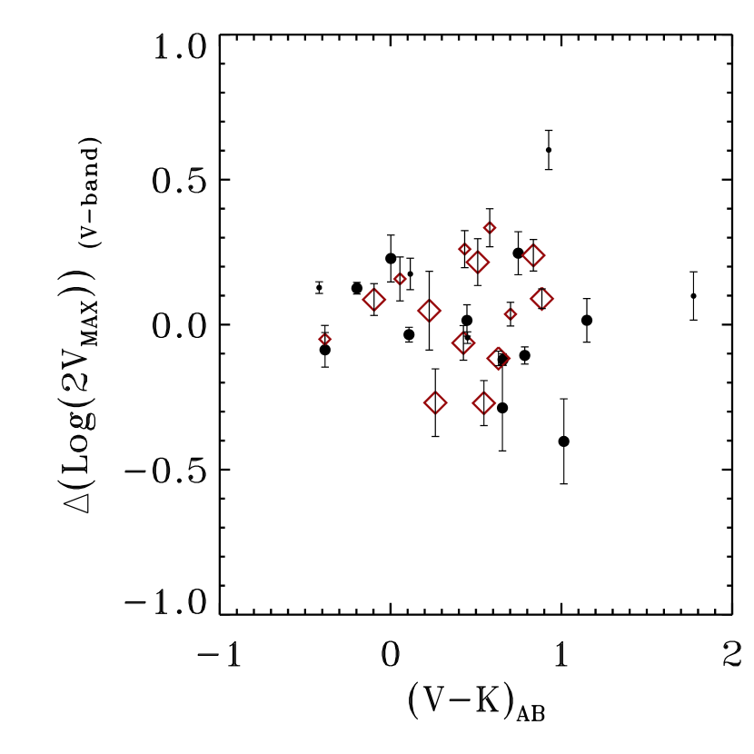
Figure 5.— The residuals from the local $V$-band Tully-Fisher relation, in the $\log(2V_{MAX})$ direction, versus rest $(V-K_{S})_{AB}$ color. Magnitudes are corrected for inclination-dependent internal extinction, as discussed in the text. Symbols are coded as in Figure 4.

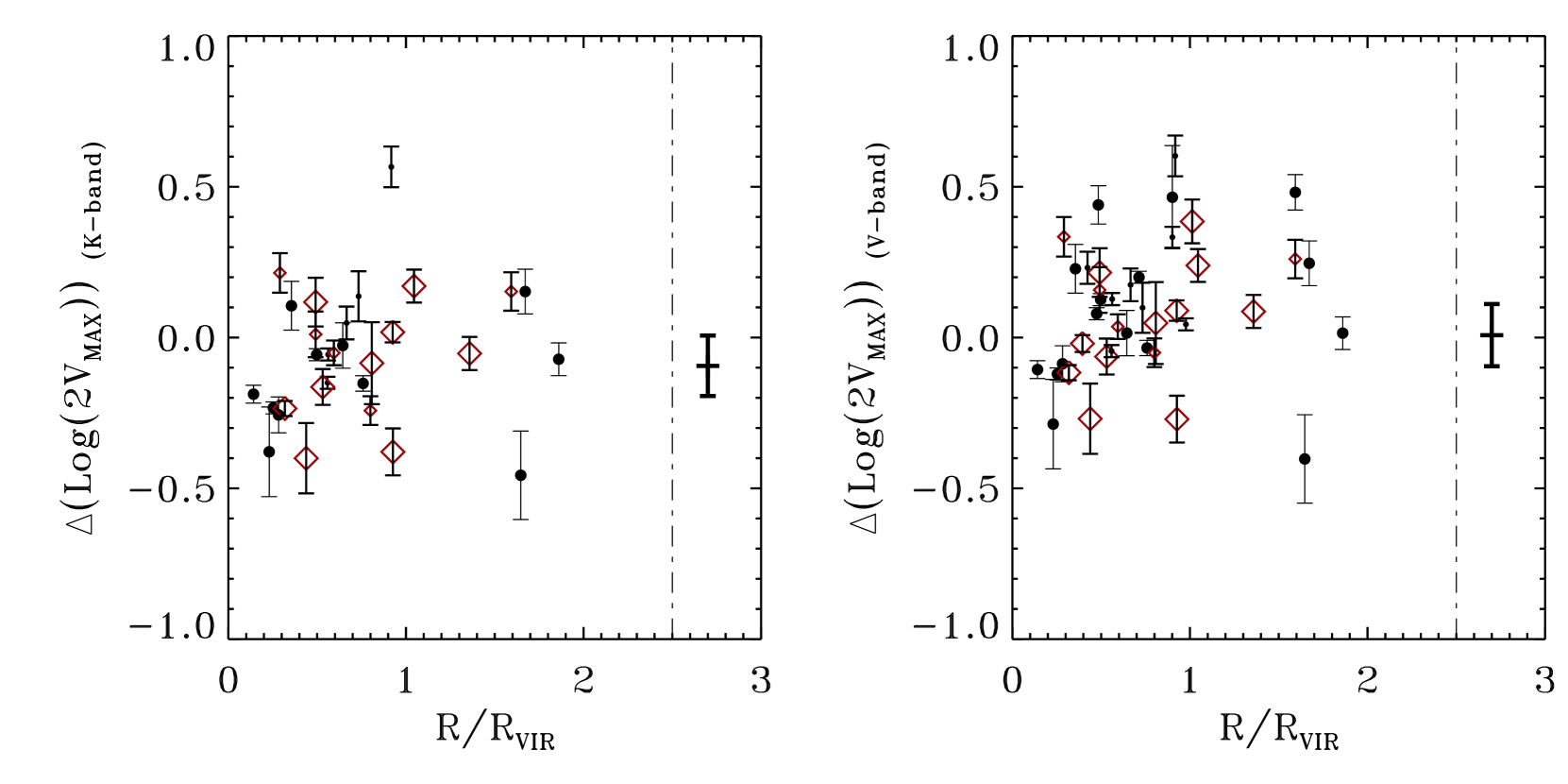
Figure 6.— The residuals from the local Tully-Fisher relation as a function of normalized projected radius, $R/R_{VIR}$. Symbols are coded as in Figure 4. Black crosses to the right of the dash-dotted line indicate the median and RMS residuals of the field TF. Positive residuals indicate that a galaxy is overluminous for its measured velocity, or, alternatively, has an anomalously low $V_{MAX}$ given its luminosity.

It is striking that such a small difference in the choice of rotation curve function can yield such a large difference in the resulting velocity value. When comparing their results to other Tully-Fisher studies, Metevier et al. (2006) take pains to comprehensively account for many of the systematic differences between studies, most having to do with the way velocities were measured or defined. They show that these small differences greatly affect estimates of the average luminosity evolution of spirals as a function of redshift. Because of the difficulty in comparing TF relations across samples, and the additional, previously under-appreciated systematic arising from the choice of rotation curve function, we do not attempt in this paper to make a rigorous estimate of the luminosity evolution implied by our TF zero point.

In fact, generally, and for our present goal of studying environmental influences on spiral galaxies, these variations between studies highlight the importance of matched samples of cluster and field spirals. Our current matched sample, which contains the largest number of cluster galaxies so far, allows us to move beyond the Tully Fisher relation, to study directly the kinematics of spirals galaxies in the hope of uncovering the source of the large scatter seen in the cluster TF relation.

5. Trends in Spiral Masses, Densities, and M/L

Movement of a galaxy in the TF plane can be caused by various effects. Increased star formation or dustiness moves a galaxy along the luminosity axis, while increased total mass, changes to the radial mass profile, or other kinematic disturbances can alter a galaxy’s measured $V_{MAX}$. In this section, we attempt to identify the source of the high scatter observed in the cluster TF, compared to the field in the same redshift range. Because our cluster sample spans a large range in cluster-centric radius, it makes sense to examine the residuals of the TF and other dynamical characteristics of the cluster spirals as a function of environment within the clusters.

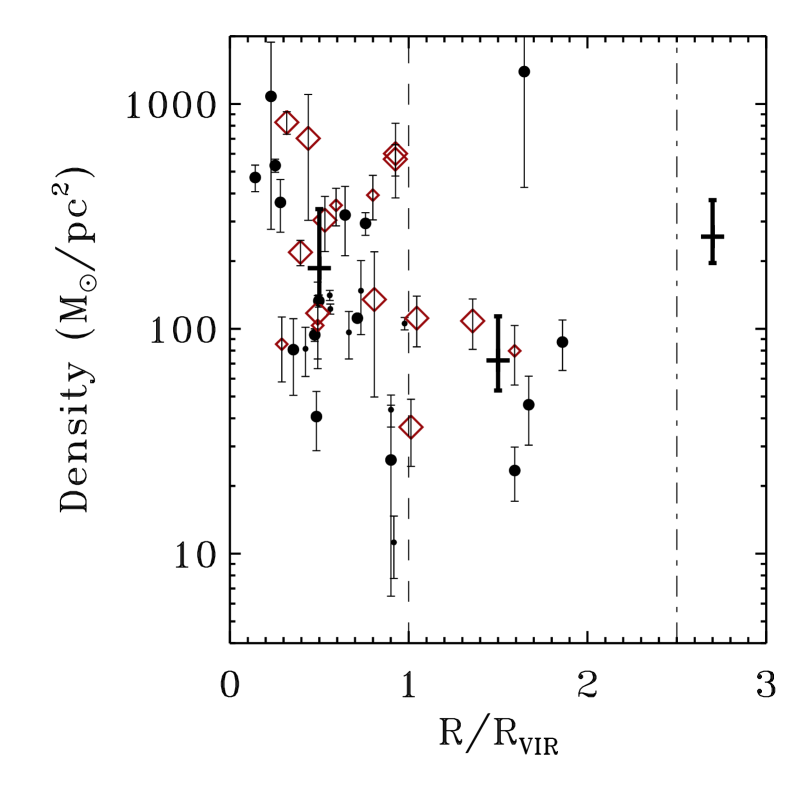
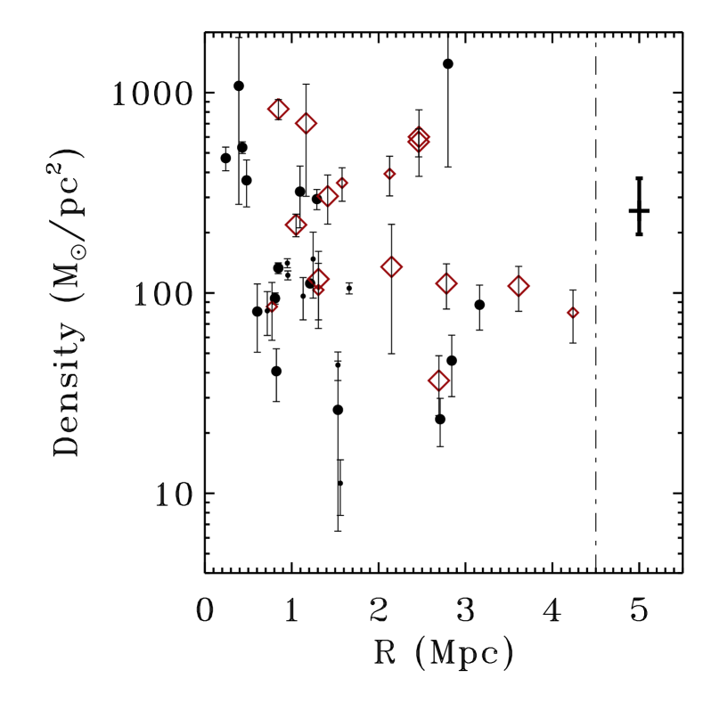
Figure 7.— Left: Projected central density of cluster spirals, measured within $1.25r_{s}$, versus projected $R/R_{VIR}$, calculated according to $\Sigma_{m}(<r)=V^{2}/(Gr)$ Right: Central density versus radius R. In both panels, The thick cross to the right of the dash-dotted line indicates the median density for our field sample. In the left panel, additional thick crosses indicate the median densities inside and outside 1 $R_{VIR}$. Symbols are coded as in Figure 4.

5.1. Tully Fisher Residuals and M/L

We first turn toward the simplest quantity to examine: the residuals from the TF, considered to represent a change in mass to light ratio (M/L). The higher scatter seen in the cluster TF, compared to the field, could plausibly be due to changes in star formation rate or dust obscuration as galaxies fall into the cluster. This could cause a radial gradient in $M/L$, which we would observe as an increased TF scatter.

However, because enhanced scatters are measured in both $V$ and $K_{S}$ band TF relations, we do not expect that the enhancement can be solely attributed to an increase or decrease in star formation or dust during cluster infall. If such a scenario were the main driver of the scatter, we would expect that the $V$-band scatter would be higher than the $K_{S}$-band, yet they are broadly equivalent. We would also expect to see a correlation between TF residuals and other indicators of star formation rate or dustiness. To test this, we plot, in Figure 5, the V-band TF residuals versus $V-K_{S}$ color for all galaxies in our cluster sample. Here, and for the rest of this paper, residuals are plotted in the sense that a positive residual is overluminous for its measured velocity, or, alternatively, has an anomalously low $V_{MAX}$ given its luminosity. No obvious correlation is observed in Figure 5. While several of our objects with lowest measured $V_{MAX}$ are not plotted here because they do not have $K_{S}$ detections, these were also excluded from the TF relation fitting, and so are not the source of the enhanced scatter.

Even though star formation rate and dust content do not appear to correlate with TF residuals, the galaxies of our cluster sample span a wide range of environments, and so we also examine whether the increased TF scatter is related to a gradient in $M/L$ across the cluster, as might be the case if spirals in the outskirts have formed more recently than those in the cluster cores. In Figure 6, we plot the TF residuals as a function of $R/R_{VIR}$, the projected cluster-centric radius scaled by each cluster’s Virial radius: 1.7Mpc for Cl 0024 (Treu et al., 2003) and 2.7 Mpc for MS 0451 (Moran et al., 2007). As MS 0451 is much more massive than Cl 0024, a galaxy at 1 Mpc radius in Cl 0024 experiences a very different environment from a galaxy at the same radius in MS 0451. As we will see below, some key trends emerge when we choose to scale by Virial radius, rather than plotting radius directly on the x-axis.

Examined by eye, the residuals from the V band TF in Figure 6 (right panel) hint at a radial gradient as a function of $R/R_{VIR}$, with galaxies at higher radius seeming to be overluminous. However, straight line fits to the $V$ and $K_{S}$ band residuals find a small gradient toward higher radius, but with slope no greater than the error bar on a typical point. A simple gradient in star formation rate or $M/L$ across the cluster therefore cannot be the only mechanism responsible for the increased scatter in the cluster TF compared to the field. We note, however, that we cannot rule out the possibility that several different mechanisms are simultaneously contributing to the TF scatter by acting on spirals in different environments within the clusters.

5.2. Densities and Masses

Since variations in star formation rate and dust content alone cannot account for the observed scatter in the cluster TF, we are led to consider the idea that the cluster spirals are more kinematically disturbed than their field counterparts. One way to test for disturbed dynamics in a spiral galaxy is to consider the photometric effective radius, $r_{s}$, of each galaxy. We can combine $r_{s}$ with $V_{MAX}$ to calculate two fundamental dynamical properties of spiral disks: dynamical mass, $M(<r)\propto V^{2}r$ and central surface mass density, $\Sigma_{m}(<r)\propto V^{2}/r$. Unlike the Fundamental Plane of ellipticals, the Tully-Fisher relation in the local universe does not seem to have any dependence on galaxy size ($r_{s}$) (e.g. Verheijen, 2001). Therefore, in an undisturbed population of spirals, we would not expect to uncover any independent environmental trends in quantities that only depend on $r_{s}$ and $V_{MAX}$. Any trends that do exist must be the result of some cluster-related physical process.

In fact, surface densities allow us to directly probe for the action of a key physical mechanism, galaxy harassment (Moore et al., 1999). Harassment is predicted to have a stronger effect on the least dense galaxies falling into a cluster, to the point of completely disrupting the most tenuous spirals. Any observed gradient in the mean density of spirals could then implicate the action of this physical process.

We choose to study M and $\Sigma_{m}$ within a radius of $1.25r_{s}$, a characteristic radius chosen because it is typically reached in all of our observed rotation curves, and it is a radius at which most of our rotation curves have already leveled off to $V_{MAX}$.

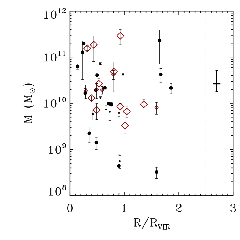
Figure 8.— Dynamical mass (within 1.25$r_{s}$) as a function of $R/R_{VIR}$, calculated according to $M(<r)=V^{2}r/G$. We find galaxies with a range of dynamical masses, both within and outside of the Virial radius. Symbols are coded as in Figure 4. The median for the field sample is displayed to the right of the dash-dotted line.

In Figure 7, we plot galaxy density as a function of projected radius R (right panel) as well as the normalized quantity $R/R_{VIR}$ (left). In the left panel, one notices a striking break in the densities of spirals at approximately $1R_{VIR}$. Near and outside of this radius, spirals seem to exhibit nearly uniformly low central densities, which are puzzlingly even lower than those of field galaxies in the sample. Within the Virial radius, on the other hand, a large spread in densities is seen, and perhaps a radial gradient of decreasing density outward from the cluster center. In the right hand panel, this trend appears scrambled, indicating that whatever physical process may cause this effect, its strength scales as the cluster Viral radius. This observation rules out several possible mechanisms, and will be discussed further in the next section.

It is natural to wonder if the observed break in density as a function of radius is due to simple luminosity segregation: if more massive spirals are found near the cluster center, perhaps these also have higher central densities. However, by consulting Figure 8, where we plot dynamical mass as a function of $R/R_{VIR}$, it becomes apparent that this is not the case. The low density spirals found in the clusters’ outskirts in fact exhibit a wide spread in total mass. Because the total number of observed spirals in the cluster outskirts is small, K-S tests comparing the distributions of mass and density for low-R vs. high-R spirals are inconclusive. However, the cluster sample as a whole does exhibit a larger overall spread in $\Sigma_{m}$ than the field sample, and includes a larger fraction of both low and high density spirals: a K-S test gives a $1.3\%$ chance that the two samples are drawn from the same parent distribution. This indicates that the cluster environment may be affecting the internal mass distributions of spirals at all cluster radii.

6. DISCUSSION

What physical mechanisms, then, could be acting on cluster spirals to reproduce both the overall higher scatter in the TF and the observed radial trend in density? The effects seem to persist as far as $2R_{VIR}$ from the cluster cores, so even though some of the observed galaxies at high radius may be part of a “backsplash population”, it is very unlikely that nearly all star forming spirals in our sample have already been through the cluster center. Therefore, we do not think it likely that tidal processes are responsible, as they are only strong near the cluster center. Instead, we can consider several proposed physical mechanisms that are strong enough at large radius to alter the dynamics of a spiral, either directly or indirectly.

In the cluster outskirts, recent mergers are an obvious candidate to drive both the large TF scatter and the abnormally low densities (e.g. Treu et al., 2003, and references therein) Mergers are less common in the low density field, and this could explain why we do not see any low-density spirals in our field sample. Unknown selection biases, though, could prevent us from including similar field galaxies in our Tully-Fisher sample. If the effects of a recent merger last for at least 1 Gyr (Bekki, 1998), then recent mergers can affect the TF scatter even in the cluster core (Treu et al., 2003). Therefore, we can not rule out the possibility that increased merging in the cluster outskirts serves to drive a high fraction of cluster spirals away from the TF relation.

In the inner regions of galaxy clusters, mergers are suppressed due to the high relative speeds of galaxies, which prevent the creation of a gravitationally bound pair during close encounters. Instead, an infalling cluster galaxy is likely to experience repeated close encounters at high speed due to the high density of galaxies in the cluster. This process, called galaxy–galaxy harassment, can lead to dramatic changes in a galaxy. Moore et al. (1999) have shown through simulations that the fate of a harassed galaxy depends on its original mass and central density. Strongly concentrated Sa/Sb type galaxies were seen to puff up their disks during infall, and so harassment may represent one way in which spirals transform into S0s in clusters. On the other hand, lower density Sc/Sd spirals are more strongly affected by harassment; Moore et al. (1999) found that they were either completely disrupted, or else transformed into an object resembling a dwarf galaxy.

If harassment is acting to transform the lowest density spirals into dwarfs, then we would expect to observe a deficit of such low-density spirals near the cluster cores. High-density spirals, on the other hand, should be more resistant to harassment, and are likely to persist to smaller cluster radii. This prediction qualitatively matches the trend in densities seen in Figure 7, but the picture is unclear. The puzzling lack of high-density galaxies at large cluster radius, and the persistence of low-density galaxies to $\sim 0.5R_{VIR}$ raise questions about this interpretation. We have already seen in Figure 8 that galaxies of a wide range of masses are represented in the cluster outskirts, so harassment alone may not present a complete explanation for the observations. Frequent mergers in the cluster outskirts, however, could very well provide the missing ingredient for keeping spiral densities low there.

Finally, we consider processes that depend on the hot intracluster medium (ICM). Generally, even strong interactions with the ICM like ram pressure stripping are thought to be too weak to explain the observed disruptions in the kinematics of spiral disks (Quilis et al., 2000). Rather, such ICM-related processes act largely to suppress star formation within infalling disks. Since changes in star formation rate do not appear to be responsible for the increased scatter in the cluster TF, it is unlikely that an ICM-related process is involved. However, it is possible that shock fronts within the ICM can enhance the ICM’s ability to affect a spiral disk even at high cluster radius (Moran et al., 2005, and references therein). Cl 0024 may be undergoing a face-on merger with a large group (Czoske et al., 2002), and so shocks may be important in this cluster. Shocks in the ICM may induce centrally-concentrated starbursts within infalling cluster galaxies (Moran et al., 2005), but it is not clear that such an interaction would generate emission lines with enough spatial extent to allow measurement of rotation curves. Further, since all ICM related processes suppress star formation over time, our sample of exclusively star-forming spirals can only provide and incomplete picture at best of the effects of ICM shocks.

One possible concern with our result on the cluster TF relation is that cluster to cluster variation could be high (as seen for example by the MORPHS and EDIScS studies, (Poggianti et al., 1999; White et al., 2005)). In fact, previous studies of Cl 0024 have shown that its galaxy population may be overly active, possibly due to the ongoing merger with a foreground large group (Czoske et al., 2002). Indeed, Moran et al. (2007) showed that the Fundamental Plane of elliptical and S0 galaxies in Cl 0024 exhibits a higher scatter than found in most other intermediate redshift clusters (Kelson et al., 2000, e.g.), though this effect is most significant in the inner 1 Mpc of the cluster. It is possible that the increased TF scatter we see is connected to the similarly enhanced Fundamental Plane scatter. However, while our cluster TF includes a majority of points from Cl 0024 (24 galaxies c.f. 16 for MS 0451), it seems clear by inspection of Figure 4 that MS 0451 also contains spirals that deviate highly from the local TF. As MS 0451 is thought to be in a more advanced stage of cluster assembly than Cl 0024 (Moran et al. 2007, in preparation), the universality of our measured TF scatter remains uncertain until similarly large samples for several more intermediate redshift clusters become available.

7. CONCLUSIONS

In this paper, we have studied the dynamics of cluster and field spirals at intermediate redshifts, via an analysis of their optical rotation curves.

We have presented one of the most complete Tully Fisher relations available for both cluster and field spirals at these redshifts, and have demonstrated that the field relation is quite tight even at these high look back times. In contrast, the cluster TF exhibits a remarkably high scatter. By comparing the trends of Tully-Fisher residuals vs radius with those in colors and local mass density we found that the increased scatter cannot be explained solely in terms of environmental effects on the star formation rates of infalling galaxies. We therefore proposed that the increased scatter in the Tully Fisher relation is due to kinematic disturbances, as expected for example for cluster harassment.

We also found a trend in galaxy mass density as a function of cluster centric radius in the sense that spiral galaxies are denser in the central regions of clusters. This is expected if harassment plays a significant role, as the densest disks would be most likely to survive during the infall. However, we found a paucity of high density spiral galaxies in the cluster outskirts, which cannot be explained by harassment alone. We suggest that a combination of enhanced merging in the cluster outskirts with galaxy harassment in the intermediate and inner cluster regions may be required to explain the observed trend in galaxy density.

Larger matched samples covering a larger number of galaxy clusters are needed to determine if the observed trends are universal across clusters at these redshifts.

Table 3Information and Measurements of Cl 0024, MS 0451 and field galaxies

Object	Sample	$z$	RA	DEC	$r_{s}$	$i$	Sl PA	$M_{V}$	$M_{K}$	$V_{\textrm{MAX}}$	Q
			[deg]	[deg]	[kpc]	[deg]	[deg]	[mag]	[mag]	[km/s]
(1)	(2)	(3)	(4)	(5)	(6)	(7)	(8)	(9)	(10)	(11)
p0i27c3	Cl0024	0.392	6.639747	17.156639	5.23	54.2	11	-21.80$\pm$0.05	-22.58$\pm$0.06	219 $\pm$ 14	1
p38i14c3	Cl0024	0.400	6.631994	17.154470	4.91	50.5	60	-21.67$\pm$0.06	-22.32$\pm$0.06	322 $\pm$ 119	1
p0i163c4	Cl0024	0.394	6.674678	17.164650	8.70	62.0	3	-22.89$\pm$0.09	-23.55$\pm$0.05	300 $\pm$ 10	1
p0i145c4	Cl0024	0.399	6.676911	17.158810	3.05	28.2	13	-20.43$\pm$0.07	-20.05$\pm$0.30	147 $\pm$ 19	1
N36671	MS0451	0.527	73.521355	-2.994348	6.68	39.6	36	-22.89$\pm$0.07	-23.47$\pm$0.05	105 $\pm$ 16	2
N37826	MS0451	0.530	73.523247	-2.988543	6.18	57.4	10	-23.12$\pm$0.06	-23.75$\pm$0.05	316 $\pm$ 18	1
p38i122c2	Cl0024	0.390	6.618957	17.155710	2.38	36.1	41	-19.84$\pm$0.06	-19.84$\pm$0.32	61 $\pm$ 11	1
N35977	MS0451	0.531	73.506584	-2.993443	3.48	67.4	13	-20.30$\pm$0.07	–	122 $\pm$ 7	1
p37i110c3	Cl0024	0.377	6.671664	17.129601	3.82	80.4	22	-20.81$\pm$0.07	–	78 $\pm$ 9	2
P51837	MS0451	0.526	73.566147	-3.065880	7.33	62.3	55	-21.77$\pm$0.08	-22.04$\pm$0.05	317 $\pm$ 90	1
p37i18c3	Cl0024	0.392	6.676580	17.128189	6.50	69.8	0	-20.75$\pm$0.05	–	109 $\pm$ 3	1
p36i29c3	Cl0024	0.400	6.616654	17.189550	2.66	79.8	29	-20.62$\pm$0.07	–	45 $\pm$ 6	1
N25094	MS0451	0.535	73.499481	-3.053076	6.24	68.7	42	-21.56$\pm$0.07	-21.61$\pm$0.06	112 $\pm$ 20	2
P62230	MS0451	0.530	73.562500	-3.073720	3.53	55.2	44	-21.21$\pm$0.06	-21.72$\pm$0.05	89 $\pm$ 16	1
p36i77c4	Cl0024	0.396	6.640263	17.205460	7.91	77.6	0	-22.22$\pm$0.06	-22.02$\pm$0.10	143 $\pm$ 4	1
P63232	MS0451	0.538	73.494949	-2.982716	4.23	47.4	28	-20.92$\pm$0.06	-21.35$\pm$0.06	158 $\pm$ 21	1
p37i2c3	Cl0024	0.377	6.676347	17.117929	10.23	75.5	0	-21.31$\pm$0.13	-21.76$\pm$0.20	167 $\pm$ 4	2
p36i37c4	Cl0024	0.388	6.630331	17.208891	4.69	69.2	1	-21.07$\pm$0.06	-20.65$\pm$0.23	105 $\pm$ 2	2
P54663	MS0451	0.541	73.597534	-3.063867	3.35	56.1	21	-21.65$\pm$0.06	-22.35$\pm$0.05	152 $\pm$ 14	2
p19i2c4	Cl0024	0.396	6.591903	17.168131	3.71	31.0	29	-21.47$\pm$0.06	-22.62$\pm$0.05	152 $\pm$ 26	1
p19i1c4	Cl0024	0.397	6.595224	17.186880	3.94	32.8	8	-20.69$\pm$0.07	-20.80$\pm$0.20	86 $\pm$ 10	2
p13i19c4	Cl0024	0.381	6.617717	17.218800	4.26	78.8	0	-21.34$\pm$0.05	–	96 $\pm$ 1	1
p23i151c2	Cl0024	0.393	6.679020	17.103390	3.02	23.8	21	-20.32$\pm$0.05	-22.09$\pm$0.06	93 $\pm$ 16	2
p18i234c4	Cl0024	0.396	6.721228	17.167561	2.55	62.9	16	-20.14$\pm$0.08	-20.25$\pm$0.29	121 $\pm$ 6	1
N27099	MS0451	0.550	73.635056	-3.040075	4.67	77.9	29	-21.73$\pm$0.06	-21.35$\pm$0.07	189 $\pm$ 21	2
N49410	MS0451	0.528	73.533180	-2.924410	8.54	35.4	53	-21.70$\pm$0.05	-21.93$\pm$0.05	150 $\pm$ 47	1
p24i55c2	Cl0024	0.388	6.639475	17.082970	1.85	71.6	27	-19.29$\pm$0.09	–	30 $\pm$ 11	1
p25i136c3	Cl0024	0.395	6.584536	17.114901	5.37	81.9	24	-21.16$\pm$0.08	–	67 $\pm$ 5	2
p24i1c2	Cl0024	0.392	6.646124	17.081320	3.19	60.4	13	-19.93$\pm$0.10	-20.85$\pm$0.24	26 $\pm$ 4	2
N46608	MS0451	0.540	73.473412	-2.938749	1.75*	61.1	21	-21.79$\pm$0.05	-22.67$\pm$0.05	139 $\pm$ 13	1
N48527	MS0451	0.544	73.488052	-2.927898	9.94	50.3	40	-22.05$\pm$0.05	-22.60$\pm$0.05	341 $\pm$ 62	1
p13i15c2	Cl0024	0.397	6.598421	17.232731	9.00	75.9	0	-21.29$\pm$0.05	–	136 $\pm$ 4	2
N34128	MS0451	0.534	73.427948	-3.003162	4.28	75.5	3	-20.84$\pm$0.06	–	55 $\pm$ 9	1
N48766	MS0451	0.551	73.469215	-2.925409	3.49	33.9	26	-21.30$\pm$0.05	-22.14$\pm$0.05	87 $\pm$ 11	1
N47732	MS0451	0.534	73.413109	-2.930732	4.23	46.3	24	-20.26$\pm$0.06	-20.17$\pm$0.15	94 $\pm$ 11	1
N64729	MS0451	0.540	73.520599	-2.835176	4.57	44.2	38	-21.37$\pm$0.06	-21.80$\pm$0.05	84 $\pm$ 12	2
p7i72c2	Cl0024	0.373	6.597922	17.299730	1.68	46.0	18	-19.04$\pm$0.07	–	27 $\pm$ 3	1
p30i4c3	Cl0024	0.393	6.552849	17.050751	5.82	35.8	54	-21.46$\pm$0.13	-22.48$\pm$0.10	398 $\pm$ 138	1
p10i41c4	Cl0024	0.396	6.801073	17.199739	13.68	41.4	30	-22.30$\pm$0.10	-23.04$\pm$0.05	110 $\pm$ 18	1
p33i308c4	Cl0024	0.382	6.603914	17.000919	7.10	46.8	26	-20.21$\pm$0.05	-20.65$\pm$0.25	110 $\pm$ 13	1
p5i171c4	field	0.313	6.742421	17.238001	3.43	74.8	0	-20.77$\pm$0.11	-21.38$\pm$0.07	99 $\pm$ 3	1
N33315	field	0.314	73.373642	-3.008564	4.16	55.8	47	-21.67$\pm$0.13	–	159 $\pm$ 29	1
N22367	field	0.325	73.610954	-3.070553	5.06	74.7	45	-21.95$\pm$0.05	-22.29$\pm$0.05	185 $\pm$ 34	1
N47194	field	0.326	73.525711	-2.939083	7.08	33.0	44	-21.81$\pm$0.06	-22.27$\pm$0.05	172 $\pm$ 43	1
N58982	field	0.326	73.631409	-2.867468	4.26	44.3	14	-20.04$\pm$0.06	-19.57$\pm$0.17	115 $\pm$ 10	1
N11649	field	0.329	73.513878	-3.123671	2.40	57.4	42	-20.53$\pm$0.07	-21.36$\pm$0.05	80 $\pm$ 14	1
N30997	field	0.333	73.444008	-3.020530	2.59	62.4	20	-20.55$\pm$0.06	-21.05$\pm$0.05	104 $\pm$ 8	1
N11932	field	0.362	73.463303	-3.124372	3.95	41.0	67	-20.96$\pm$0.06	-21.27$\pm$0.05	235 $\pm$ 133	1
N48819	field	0.363	73.460930	-2.927250	1.93	28.1	26	-20.41$\pm$0.05	-21.16$\pm$0.05	83 $\pm$ 10	2
N55288	field	0.364	73.419220	-2.892889	5.20	62.6	50	-20.56$\pm$0.06	-20.23$\pm$0.08	113 $\pm$ 17	2
N37713	field	0.367	73.467995	-2.987958	4.95	27.2	0	-21.06$\pm$0.05	-21.91$\pm$0.05	204 $\pm$ 20	1
N21079	field	0.371	73.350967	-3.074297	2.86	42.9	33	-20.45$\pm$0.05	-21.42$\pm$0.05	118 $\pm$ 18	1
N31950	field	0.371	73.444237	-3.017617	3.69	55.2	41	-21.43$\pm$0.05	-22.03$\pm$0.05	182 $\pm$ 32	1
N35309	field	0.390	73.625328	-2.996757	3.32	66.3	21	-21.18$\pm$0.05	-21.51$\pm$0.05	131 $\pm$ 11	1
N57426	field	0.391	73.473892	-2.878548	3.73	60.3	38	-21.66$\pm$0.05	-22.98$\pm$0.05	274 $\pm$ 43	1
N18456	field	0.401	73.598076	-3.087556	4.13	61.0	14	-21.55$\pm$0.05	-22.13$\pm$0.05	182 $\pm$ 11	1
N35519	field	0.413	73.426918	-2.997052	3.83	40.8	43	-20.43$\pm$0.05	-20.76$\pm$0.06	135 $\pm$ 27	2
N19992	field	0.419	73.515671	-3.081446	6.52	51.5	4	-21.36$\pm$0.20	–	121 $\pm$ 11	1
N18483	field	0.425	73.465881	-3.088012	4.56	71.7	3	-22.18$\pm$0.05	-22.83$\pm$0.05	177 $\pm$ 6	1
p17i129c4	field	0.443	6.766013	17.151690	10.24	84.6	2	-22.69$\pm$0.07	-21.99$\pm$0.20	215 $\pm$ 3	2
N36846	field	0.447	73.670662	-2.991703	2.73	45.3	0	-21.60$\pm$0.05	-22.75$\pm$0.05	180 $\pm$ 11	1
N40959	field	0.447	73.624619	-2.969724	3.40	34.8	13	-22.12$\pm$0.05	-22.88$\pm$0.05	187 $\pm$ 19	1
N41465	field	0.447	73.629173	-2.963893	4.67	74.7	21	-21.33$\pm$0.05	-20.84$\pm$0.08	142 $\pm$ 11	1
N56286	field	0.463	73.505577	-2.884414	4.59	53.6	3	-21.53$\pm$0.05	-21.70$\pm$0.05	209 $\pm$ 10	1
p11i11c4	field	0.476	6.724503	17.193130	2.77	27.3	18	-20.51$\pm$0.09	-20.69$\pm$0.27	74 $\pm$ 13	1
N25636	field	0.491	73.394081	-3.050711	6.04	28.5	15	-21.67$\pm$0.06	-22.66$\pm$0.05	174 $\pm$ 22	2
p8i163c3	field	0.492	6.569071	17.296320	3.14	56.7	7	-20.97$\pm$0.10	-21.55$\pm$0.19	128 $\pm$ 5	1
N59564	field	0.494	73.547920	-2.870288	4.66	71.4	22	-22.00$\pm$0.05	-22.16$\pm$0.05	172 $\pm$ 15	1
p1i97c4	field	0.494	6.770693	17.324760	3.00*	38.8	16	-21.59$\pm$0.06	-22.20$\pm$0.12	59 $\pm$ 8	2
N11338	field	0.505	73.540504	-3.126556	5.12	36.2	33	-21.76$\pm$0.06	-22.80$\pm$0.05	258 $\pm$ 45	1
N25124	field	0.506	73.698349	-3.052146	7.84	39.4	44	-21.90$\pm$0.06	-22.83$\pm$0.05	194 $\pm$ 45	1
p23i180c2	field	0.536	6.677425	17.101549	5.56	56.0	14	-21.26$\pm$0.07	-22.08$\pm$0.14	146 $\pm$ 10	1
p21i99c3	field	0.537	6.475233	17.202730	2.68	36.1	3	-20.93$\pm$0.05	-20.97$\pm$0.28	157 $\pm$ 14	1
N37427	field	0.579	73.516296	-2.988545	5.59	31.0	43	-22.45$\pm$0.06	-23.48$\pm$0.05	215 $\pm$ 53	1
p34i20c3	field	0.595	6.533985	16.984360	4.26	53.3	2	-21.15$\pm$0.05	-21.06$\pm$0.32	109 $\pm$ 7	1
N41286	field	0.600	73.466621	-2.966479	2.53	43.0	22	-21.33$\pm$0.05	-20.67$\pm$0.11	107 $\pm$ 12	1
p34i94c2	field	0.614	6.553948	16.984819	11.47	38.2	30	-21.23$\pm$0.07	-21.58$\pm$0.33	251 $\pm$ 37	2

Note. — Cluster galaxies are arranged in order of increasing $R/R_{VIR}$, where $R_{VIR}=1.70$ Mpc for Cl 0024 and $R_{VIR}=2.66$ for MS 0451. The cluster centers are (6.6500,17.1433) and (73.5454,-3.0186) J2000, for Cl 0024 and MS 0451, respectively. Field galaxies are arranged in ascending redshift order. Col. (1): Object name. Col (2): Indicates which subsample that each galaxy belongs to: Cl 0024, MS 0451, or field. Col (3): Redshift of each galaxy. Cols (4) and (5): J2000 coordinates for each galaxy. Cols (6) and (7): Scale lengths $r_{s}$ and inclinations $i$ measured via GALFIT. $i=90^{\circ}$ indicates edge-on. * Denotes objects where $R_{S}$ was set manually to improve the fit. Col (8): Indicates the misalignment between the PA of the spectroscopic slit and the major axis of the galaxy. Typical formal errors on $r_{s}$, $i$, and Sl PA are 10$\%$, $0.5^{\circ}$, and $1^{\circ}$, respectively; systematic uncertainties in $i$ and Sl PA are typically $\sim 10^{\circ}$. Cols (9) and (10): Absolute magnitudes in rest-frame V and K bands, corrected for inclination-dependent internal extinction. Col (11): Measured $V_{MAX}$. In cases where more than one emission line was measured, this is a weighted average. Col (12): Rotation curve quality. $Q=1$ curves display turnovers on both ends; Q=2 curves display only one turnover, or an uncertain fit.

References

- Bamford et al. (2006) Bamford, S. P., Aragon-Salamanca, A. & Milvang-Jensen, B. 2006, MNRAS, 366, 308
- Bamford et al. (2005) Bamford, S. P., Aragon-Salamanca, A., Milvang-Jensen, B. & Simard, L. 2005, MNRAS, 361, 109
- Bekki (1998) Bekki, K. 1998, ApJ, 502, L133
- Bertin & Arnouts (1996) Bertin, E. & Arnouts, S. 1996, A&AS, 117, 393
- Blanton et al. (2003) Blanton, M. R., Brinkmann, J., Csabai, I. et al. 2003, AJ, 125, 2348
- Böhm et al. (2004) Böhm, A., Ziegler, B., Saglia, R. et al. 2004, A&A, 420, 97
- Cuillandre et al. (2000) Cuillandre J.-C., Luppino, G., Starr, B., & Isani, S. 2000, Proc. SPIE.4008, 1010
- Czoske et al. (2002) Czoske, O., Moore, B., Kneib, J.-P., & Soucail, G. 2002, A& A, 386, 31
- Davis et al. (2003) Davis, M., Faber, S., Newman, J. et al. 2003, SPIE, 4834, 161
- Dressler et al. (1997) Dressler, A., Oemler, A., Jr., Couch, W. J. et al. 1997, ApJ, 490, 577
- Kannappan et al. (2002) Kannappan, S. J., Fabricant, D. G. & Franx, M. 2002, AJ, 123, 2358
- Kelson et al. (2000) Kelson, D. D., Illingworth, G. D., van Dokkum, P. G., & Franx, M. 2000, ApJ, 531, 184
- Kodama et al. (2005) Kodama, T., Tanaka, M., Tamura, T. et al. 2005, PASJ, 57, 309
- Metevier et al. (2006) Metevier, A., Koo, D., Simard, L. & Phillips, A. 2006, ApJ, 643, 764
- Milvang-Jensen et al. (2003) Milvang-Jensen, B., Arag n-Salamanca, A. Hau, G., J rgensen, I. & Hjorth, J. 2003, MNRAS, 339, 1
- Moore et al. (1999) Moore, B., Lake, G., Quinn, T. & Stadel, J. 1999, MNRAS, 304, 465
- Moran et al. (2007) Moran, S. M. et al. 2007, in preparation
- Moran et al. (2005) Moran, S. M., Ellis, R. S., Treu, T., Smith, G. P., Smail, I., Dressler, A., Coil, A. L. 2005, ApJ, 634, 977
- Nakamura et al. (2006) Nakamura, O., Aragon-Salamanca, A., Milvang-Jensen, B., Arimoto, N., Ikuta, C & Bamford, S. P. 2006, MNRAS, 366, 144
- Peng et al. (2002) Peng, C., Ho, L., Impey, C., Rix, H. 2002, AJ, 124, 266
- Poggianti et al. (1999) Poggianti, B. M., Smail, I., Dressler, A. et al. 1999, ApJ, 518, 576
- Quilis et al. (2000) Quilis, V., Moore, B., & Bower, R. 2000, Science, 288, 1617
- Schechter (1980) Schechter, P. L., 1980, AJ, 85, 801
- Schlegel et al. (1998) Schlegel, D.J., Finkbeiner, D. P., & Davis, M. 1998, ApJ, 500, 525
- Smith et al. (2005) Smith, G. P., Treu, T., Ellis, R. S., Moran, S. M., Dressler, A. 2005, ApJ, 620, 78
- Treu et al. (2003) Treu, T., Ellis, R. S., Kneib, J. et al. 2003, ApJ, 591, 53
- Tully & Pierce (2000) Tully, R. B., & Pierce, M. 2000, ApJ, 533, 744
- Tully et al. (1998) Tully, R. B., Pierce, M., Huang, J., Saunders, W., Verheijen, M., & Witchalls, P. 1998, AJ, 115, 2264-2272
- Tully & Fouque (1985) Tully, R. B. & Fouque, P. 1985, ApJS, 58, 67
- Tully & Fisher (1977) Tully, R. B. & Fisher, J. R. 1977, A&A, 54, 661.
- Verheijen (2001) Verheijen, M. 2001, ApJ, 563, 694
- Vogt et al. (1996) Vogt, N., Forbes, D. Phillips, A., Gronwall, C., Faber, S. M., Illingworth, G., & Koo, D. 1996, ApJ, 465L, 15
- White et al. (2005) White, S., Clowe, D., Simard, L. et al. 2005, A& A, 444, 365
- Willick (1994) Willick, J. 1994, ApJS, 92, 1
- Wilson et al. (2003) Wilson, J. C., Eikenberry, S., Henderson, C. et al. 2003, Proc. SPIE, 4841, 451