Solar Resonant Diffusion Waves as a Driver
of Terrestrial Climate Change
Robert Ehrlich
George Mason University
Fairfax, VA 22030
rehrlich@gmu.edu
January 4, 2006
ABSTRACT
A theory is described based on resonant thermal diffusion waves in
the sun that explains many details of the paleotemperature
record for the last 5.3 million years.
These include the observed
periodicities, the relative strengths of
each observed cycle, and the sudden emergence in time for the 100
thousand year cycle. Other prior work suggesting a link between
terrestrial paleoclimate and solar luminosity variations has not
provided any specific mechanism. The particular mechanism described
here has been demonstrated empirically, although not previously
invoked in the solar context. The theory, while not without its own
unresolved issues, also lacks most of the
problems associated with Milankovitch cycle theory.
I paleotemperature data
The possibility that fluctuations in solar luminosity may be responsible for changes in global temperatures has not been overlooked by researchers,(Lean,1997) although most explanations for periodicities in paleotemperatures are believed to involve factors unrelated to solar luminosity.(Zachos,2001) Nevertheless, some researchers have suggested that periodic solar variability has been the cause of global temperature cycles, with periods ranging from the 11 year sunspot period to cycles as long as 2000 years.(Hu,2003) Earlier reports, however, suggest no specific mechanism for long term solar periodicity.
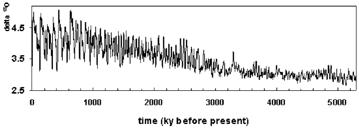
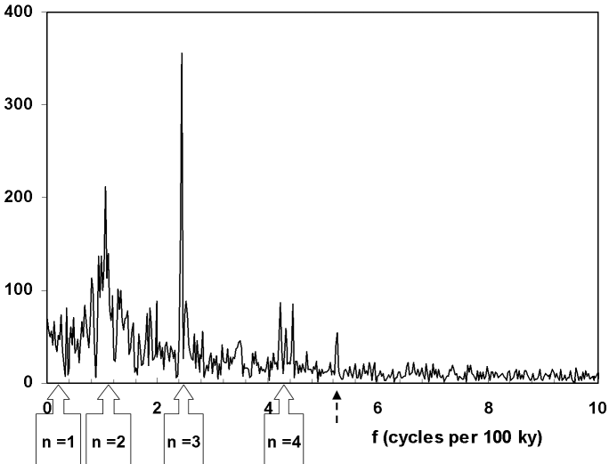
Paleotemperatures are inferred from the ratio found in benthic sediments and in ice cores versus depth. In particular, it is believed that a 5 decrease in global temperature corresponds to a 0.1% increase in the ratio (i.e., delta ) in benthic sediments.(Lisiecki,2005) Fig. 1 shows a compilation by Lisiecki and Raymo(Lisiecki,2005) who stacked 57 sets of data on benthic sediments that cover 5.3 million years (My) before present. Figs. 2 and 3 show the Fourier amplitude spectra.
II Diffusion Waves
Diffusion waves are an established phenomenon which has been studied theoretically and experimentally,(Mandelis,2000) and even for heat transport in magnetized plasmas.(Reynolds,2001) They can occur for any process, such as heat flow when a time-dependent source is present, in which case, the waves represent propagating temperature fluctuations, , and they must satisfy the diffusion equation. Assuming a sinusoidal time dependence, and separating into space and time dependent parts, we find that satisfies:
| (1) |
where is the space-dependent part of a source term, and where the complex wave number satisfies
| (2) |
Note that according to eq. 2, the imaginary (attenuation) part of the complex wave number and the real (oscillatory) part are equal, implying equality of penetration depth , and wavelength , so higher frequency waves are more severely damped. For a uniform thermal diffusivity and a spherically symmetric source eq. 1 yields the solution
| (3) |
For the more general case of an isotropic medium in which is dependent only on radial distance to the origin the same solution applies, but must now be replaced by its average value between the source radius and the r at the wave location, i.e.,
| (4) |
III The solar interior
Solar physicists use a Standard Solar Model (SSM) to calculate many properties of the sun’s interior. According to the SSM, the three interior regions of interest here are: (1) the core (of radius about 25% of the solar radius ) where fusion occurs, (2) the surrounding radiative zone (extends to about ), and (3) the surrounding convection zone, where heat makes its way to the surface by the much more rapid process of convective flow. The fairly sharp boundary layer between the radiative and convection zones is known as the “tachocline.”
Normally, one associates diffusivity with heat flow by conduction, whereas radiation is taken as a line-of-sight transmission process. However, inside the sun where the mean free path for photons between emission and subsequent reabsorption is very short (typically several millimeters), the diffusion description is applicable. Obviously, radiation is the dominant heat transfer process inside the core and radiative zones, owing to the high temperatures there, and the dependence on radiative emission and absorption rates. The diffusivity parameter depends on a variety of other quantities that govern the likelihood of photons being radiated and reabsorbed. In particular, it can be shown that the thermal diffusivity at any radial distance as (Miesch, 2005): , where is the Stefan-Boltzmann constant, is the absolute temperature, is the opacity, is the density, and is the specific heat. Each of the parameters in the previous equation can be found as a function of radial distance using data from the GONG collaboration (Christensen-Dalsgaard,1996).
Within the SSM description, the solar core is considered to be in a state of quasistatic equilibrium changing only on a timescale of 30 million years. However, Grandspierre and Agoston have noted, instabilities can be generated in a rotating plasma in the presence of a magnetic field, and these instabilities can give rise to thermal fluctuations, and heat waves that represent deviations from SSM’s.(Grandpierre,2005) They further show that constraints on the size of the core magnetic field (Friedland,2004),(Gough,1998) are such that fluctuations can indeed arise, as a natural consequence of the nonlinearity of the MHD equations.
These thermal fluctuations in the form of hot ”bubbles” tend to expand, rise, and cool on timescales Grandspierre and Agoston have estimated, which are a function of their spatial extent and the magnitude of their temperature excess.(Grandpierre,2005) Were the bubbles to remain small and isolated, the diffusion waves emanating from these fluctuations would tend to cancel each other out. However, Grandspierre and Agoston have shown that the bubbles tend to merge and grow in size, and the decay time of the waves can grow even longer than years, as the perturbations smooth out to include ever larger regions – in effect making the solar core a region of small amplitude thermal oscillations, instead of the quiescent state normally assumed.(Grandpierre,2005)
IV Description of the theory
We postulate small random variations in the temperature of the outer solar core (between and ),(Ferro,2005) which are sufficiently smoothed out, so as to be a function only of radial distance. The specific noise spectrum is unimportant, except that the noise frequencies should have slowly changing phases over times on a scale of .
Each of the noise frequencies may be thought of as a source of radially symmetric diffusion waves. When a wave reaches the tachocline, it is reflected back to the core as an ingoing wave. However, it should be noted that reflections in the case of diffusion waves are not of the usual type, where well-defined wavefronts are involved, but only resemble conventional wave reflections in the high frequency or long path-length limit (Mandelis,2001). Otherwise, a considerable amount of “phase smearing” prevents us from describing the reflection of discrete wavefronts. At a boundary, such as the tachocline, the depletion or accumulation of photons (and the associated radially symmetric periodic temperature fluctuation), creates an inward travelling diffusion wave. This inward wave interferes with the next outgoing wave produced at that frequency, and a new outward wave is generated from a superposition of the two waves. Again, however, the interference process is not one of simply superimposing well-defined wavefronts, which do not exist here. Instead, if the inward and outward waves both correspond to a maximum positive or negative fluctuation in photon density (i.e., have have matched phases), the resultant temperature fluctuation would be greatest, and hence resonance would be achieved. To achieve resonance the ingoing wave must arrive back at the core in phase with the next source cycle at this frequency, or more generally after n cycles. Thus, the condition for resonance for the nth mode is:
| (5) |
where n =1,2,3,…, and 2r is the round trip distance travelled by the wave from emission to absorption back at the core. From eq. 5 we see that the period of the nth resonant mode , so that
| (6) |
with the period of the lowest frequency resonant mode being twice the diffusion time for photons to undergo a random walk through the radiation zone before they reach the tachocline. Fortunately, can be calculated from the sun’s internal density and opacity (both functions of radial distance r) using data from the SSM.(Christensen-Dalsgaard,2005) One the most widely-cited estimates of from Mitalas and Sills(Mitalas,1992) is . We have repeated their calculation, and obtained 190 ky. In what follows, we shall use a value that brackets these two: .
Using eq. 6 we find the predicted periods for the nth resonant mode:
| (7) |
Some of the periods (for n = 2, 3 and 4) given by eq. 7 correspond to reported periods in the paleotemperature data – see markers in fig. 2. But before we can have confidence that resonant solar diffusion waves may offer an explanation of periodic variations in paleotemperatures, we must address several key issues, including whether it is possible for the waves to attain a large degree of resonant amplification.
Damping of diffusion waves Given that a diffusion wave for the nth resonant mode has a phase of on returning to the source, it will have been heavily damped, and will have an intrinsic damping:
| (8) |
The large damping of diffusion waves might seem to make the possibility of their playing a role in any resonant amplification process in the sun remote. For example, given a damping for a wave after one round trip, the next outgoing wave has an amplitude , and hence the number of cycles required for the amplitude of the nth mode to double is given as yielding doubling times in ky for mode n: . For we find doubling times that are longer than the age of the sun – even if diffusion waves are reflected 100% from the tachocline. Yet the doubling times are lengthened even more, because of damping due to “blurry boundaries,” since fractions of an outgoing wave are reflected back from different parts of the tachocline, and return to different parts of the core. Based on the relevant layer thicknesses, we find a phase smearing of the nth mode: . This additional damping, which increases with n, makes it impossible for modes to survive.
Gain due to fusion amplification. There is a compensating amplification effect that more than offsets the enormous damping, and allows resonant diffusion waves to emerge with large amplitude in a relatively few cycles. According to the SSM, the rate of nuclear fusion in the core of the sun (and hence solar luminosity ) is proportional to for small deviations from the ambient core temperature.(Bahcall,2001) To see the effect of this large exponent in amplifying diffusion waves, consider an outgoing wave for mode n initially created due to a positive core temperature fluctuation at radius . In advancing a small distance outward, the wave amplitude is reduced by . However, if the wave is absorbed by the core, it elevates the core temperature at that r by the same amount, and hence raises the luminosity there by a 4.2-fold greater fraction, due to the relationship. Thus, there is a net gain in wave amplitude over this distance of . The amplification factor multiplies the size of the temperature fluctuation, and it occurs virtually instantaneously on a diffusion time scale, so that the amplification looks like a coherent radiation wave superimposed on a much slower moving thermal wave of the same frequency. As the wave proceeds outward through the outer core, it continues to produce an ever increasing amount of thermal radiation, owing to the continual increase in luminosity. Upon reaching the edge of the core () the nth resonant mode (and the core temperature) has been amplified by a gain:
| (9) |
where can be found using eqs. 2, 4, 5, with and . The same mechanism operates for the negative portion of the wave cycle, and it amplifies reductions in core temperature. This amplification mechanism is similar to the exponential increase in intensity in the case of lasing, except that here (1) fusion makes optical pumping unecessary, and (2) the spherical symmetry assures that there is no loss of waves “out the sides,” as occurs in a laser. Evaluating eq. 9 numerically using SSM data yields .
Such a large gain (more than offsetting the damping) cannot be taken as a realistic indicator of how large the wave can grow before it leaves the core, but it does suggest that a wave might be able to resonantly attain its maximum value after only a few cycles. It should be noted that a very similar resonance phenomenon to that described here – but without any fusion gain – has been seen empirically in thermal-wave cavity environments.(Shen,1995)
Obviously, the theory provided here, which ignores nonthermal magnetic interactions, and assumes an initial temperature fluctuation that is only a function of radial distance is highly simplified. Far more numerous non-spherically symmetric temperature fluctuations would not result in a similar amplification process, and hence they will become relatively less intense over time. However, both the nonspherically symmetric fluctuations and the magnetic interactions must be considered for a full understanding of losses and gains, so as to permit a determination of the maximum steady state radial wave amplitude.
V Comparison of Between Theory and Paleoclimate Data
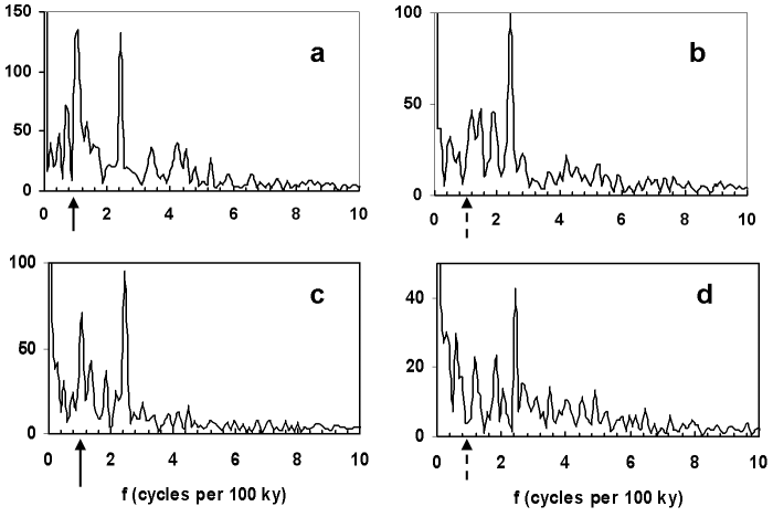
Periods of each mode. As fig. 2(markers) and table 1 show, the Fourier amplitude spectrum for the data shows peaks at the theory’s predicted modes n = 2,3 and 4. The overall data with a fifth order background subtraction to eliminate low frequency leakage shows no indication of the n = 1 mode in fig. 2. With no background subtraction there is a non-statistically significant suggestion of a peak corresponding to this mode in fig. 3(c) and especially (d), which together correspond to the interval 2048 to 4095 years before present. Were it present, a n = 1 peak (located at f = 0.28 cycles per 100 ky) could not easily be distinguished from a steeply rising low frequency background.
No periodicities predicted by the model are clearly absent from the data. It is true, however, that one small peak seen in the overall spectrum (but not in the quartile spectra) with a period of 19 ky (dotted arrow in fig. 2) is not predicted by the theory, and it cannot be the n = 5 mode which should be at 14.8 ky were its predicted amplitude not zero. Obviously, we cannot exclude the possibility that other mechanisms, including Malinkovitch cycles, play some role in paleotemperature periodicity.
Signal emergence times. By the signal “emergence time” we refer to the amount of time required for the nth mode amplitude to rise from the modest level of the background noise to a large enough multiple for it to be clearly seen in the paleotemperature record. Owing to the large gain, this amplification could occur in a few cycles according to the theory. We can determine the emergence time from the data only for modes that turn on after being off for a while. Only one of the modes (i.e., n = 2 with a 90 to 100 ky period) clearly shows this behavior, since as seen in fig 3, it is present only in the first and third time quartiles (solid arrows). It is not easy to tell from fig 1 exactly where in the vicinity of 1000 ky before the present this mode begins to appear, and just how sudden is that appearance.
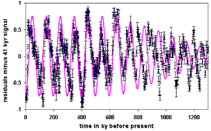
The shape of the n = 2 cycle, and the abruptness of its emergence can be gleaned by looking at the data for the most recent 1000 ky, after making a subtraction of the 41 ky cycle – see fig 4. The figure also shows vertical error bars on the original data, and a 100 ky cycle drawn to guide the eye. When the data is displayed in this manner the 100 ky cycle appears much more consistent with a sinusoidal shape than the original data for the last 1000 ky.
It can easily be seen in fig. 4 that the n = 2 mode appears fairly suddenly (between 800 and 900 ky before the present), following what appears to be a sudden phase reversal or discontinuity. If this discontinuity is real, the theory has no obvious explanation for it. However, a short emergence time is consistent with the theory, so this behavior offers some support.
Relative amplitude (and shape) of each mode.
We have addressed the issue of the lack of a clear signal for the n = 1 mode, and the non-appearance of modes with . Can the theory account for the relative amplitude (and shape) of the three other modes (n = 2,3,4) that are clearly seen in the data? It can with the aid of two further assumptions: (1) all modes have the same intrinsic strength (as a multiple of the background) when they are active, and (2) only the n = 3 mode is active most of the time.
n = 2 mode (90 ky period). A look at figs. 3(a) and (c), i.e., times when both the n = 2 and 3 modes were active, shows that the two peaks have comparable strengths. (The position of the n = 2 mode is flagged by solid and dotted arrows for those quartiles that it appears to be “on” and “off.”) Thus, the decreased size of this mode in the overall data is apparently less a matter of the differences in the intrinsic strength of each mode than what fraction of the time this mode is active. The broadening of this peak may also be attributed to its being off perhaps half the time.
n = 3 mode (40 ky period). This mode is the dominant (and narrowest) one in the overall record because it is active at all times – see figs. 3(a)through (d).
n = 4 mode (22.5 ky period). This mode is not clearly seen in the separate quartile spectra (figs. 3(a)through (d)). However, the fact that it appears to be split in the overall spectrum (into two frequency peaks separated by about 7%) has a possible explanation that relates to a single frequency turning on and off in a periodic manner. For example, if we perform a Fourier Transform on a sinusoidal signal that turns off and on say every 14 cycles, we would indeed get two separate peaks in the frequency domain separated in frequency by 7%. This phenomenon is not due to a defect of the Fourier Transform, but rather that two nearby frequencies will produce beats which mimic a single frequency turning on and off periodically. It may simply be a coincidence, but this number of cycles on and off for the n = 4 mode is close to what is seen for the n = 2 mode, which appears to be alternately on and off for approximate intervals of 1028 ky ( cycles).
Finally, how to explain the smallness of the n = 4 peak compared to n = 3? Its splitting into two separate peaks is partly responsible, as is the fact that this mode is active only a fraction of the time, unlike the n = 3 mode. A third reason for the lower n = 4 amplitude is that the damping of this mode due to blurry boundaries (twice as serious for n = 4 than n = 3) operates mainly as the amplification process is occurring while the wave travels through the core, which has the effect of preventing the n = 4 mode from reaching a large amplitude.
Can the oscillations become large enough?
The dominant (n = 3) mode seen in the Fourier spectrum (fig.2) is seen to have a signal to background ratio of about 3.4. This implies that the background noise at that frequency had to be resonantly amplified by this same factor. Given that the complex interactions with the magnetic field that might determine an upper limit to the size of the oscillations remains to be worked out, it is unclear if a 3.4-fold growth (at this particular frequency) is achievable. This unresolved issue does represent a current shortcoming of the theory.
VI Problems with Milankovitch theory and conclusion
In Milankovitch theory past glaciations are assumed to arise from small
quasiperiodic changes in the Earth’s orbital parameters that give
rise to corresponding changes in solar insolation, particularly in
the polar regions. A brief discussion of five problems with this
theory are listed below, and a more detailed description of some of
them can be found
elsewhere.(Karner,2000)
(a) Weak forcing problem: The basic problem with the theory
s that observed
climate variations are much more intense than the insolation changes
can explain without postulating some very strong positive feedback
mechanism.
(b) 100 ky problem: The preceding basic problem can be illustrated for the
case of one particular parameter – the orbital eccentricity. The dominant climate cycle observed during the
last million years has a roughly 100 ky period, which in Milankovitch theory is
linked to a 100 ky cycle in the eccentricity.
However, the effect of this eccentricity variation should be the
weakest of all the climate-altering changes, in view of the small
change in solar insolation it would cause. For example, consider the Earth’s
orbital eccentricity, e, which has been shown to have several periods
including one of 100 ky during which e varies in the approximate
range: (Quinn,1991) The resultant solar irradiance
variation found by integrating over one orbit for each of the two extreme
e-values is about , or difference
at the top of the Earth’s atmosphere. Given that climate models show that
a one percent change in solar irradance would lead to a
average global temperature change, then the change resulting from
a irradiance change would be a miniscule hardly
enough to induce a major climate event – even with significant
positive feedback.
(c) 400 ky problem: The variations in the Earth’s orbital
eccentricity show a 400 ky cycle in addition to the 100 ky cycle, with
the two cycles being of comparable strength. Yet, the record of
Earth’s climate variations only shows clear evidence for the latter.
(d) Causality problem: Based on a numerical integration of
Earth’s orbit, a warming climate predates by about 10,000 years the
change in insolation than supposedly had been its cause.
(e) Transition problem: No explanation is offered for the
abrupt switch in climate periodicity from 41 ky to 100 ky that is
found to have occured about a million years ago. Of these five
problems with Milankovitch theory, the current theory clearly shares
only (c).
In conclusion, We have here suggested a specific mechanism involving diffusion waves in the sun whose amplitude should grow very rapidly due to an amplification provided by the link between solar core temperature and luminosity. Moreover, the phenomenon of resonant amplification of thermal diffusion waves has been empirically demonstrated, albeit not in the solar context.(Shen, 1995) A number of features of the theory still remain to be resolved, but the theory does explain many features of the paleotemperature record, and it appears to be free of most defects of the Milankovitch theory. The theory further implicitly suggests the existence of a new category of variable stars having extremely long periods – i.e., times longer than stellar periods currently considered to be “very long.” For some stars with , their thinner radiation zones might make the predicted periods observable.
References
(Bahcall,2001) According to the SSM, the CNO cycle contributes 1.5% of the sun’s luminosity, with the remainder due to the pp chain – see: Bahcall,J.N., Pinsonneault, M.H., and Basu, S. “Solar Models: current epoch and time dependences, neutrinos, and helioseismological properties,” Ap. J., 555, 990-1012 (2001). At the ambient solar core temperature, these reactions have a luminosity dependence on core temperature that varies as of the form , where N is approximately 4 and 15, respectively To find the overall dependence on temperature, we may compute numerically the derivative after weighting the two reactions by their respective abundances, giving N = 4.2.
(Christensen-Dalsgaard,1996) Christensen-Dalsgaard, J., The current state of solar modeling. Science, 272, 1286-1292 (1996).
(Ferro,2005) Ferro and Lavagno have shown that it is not the entire core of the sun that is in a metastable state, but only its outer region, i.e., . See – Ferro, F., Lavagno,A., Quarati,P. “Metastable and stable equilibrium states of stellar electron-nuclear plasmas,” Phys. Lett., A336, 370-377 (2005).
(Friedland,2004) Friedland, A. and Gruzinov, A., “Bounds on the Magnetic Fields in the Radiative Zone of the Sun,” Ap. J. 601, 570–576 (2004).
(Gough,1998) Gough, D.O., and MacIntyre,M.E., “Inevitability of a magnetic field in the Sun’s radiative interior,” Nature 394, 755 (1998).
(Grandpierre,2005) Grandpierre, A. and Agoston, G.: “On the onset of thermal metastabilities in the solar core,” Astrophysics and Space Science, 298(4): 537-552 (2005).
(Hu,2003) Hu, F. S. et al., “Cyclic Variation and Solar Forcing of Holocene Climate in the Alaskan Subarctic,” 301, (5641), 1890 - 1893 (2003); Van Geel, B., “The Role of Solar Forcing Upon Climate Change, Quaternary Sci. Rev., 18, 331–338 (1999).
(Karner,2000) Karner, D.B., and Muller, R.A.,“Paleoclimate: A causality problem for Milankovitch,” Science, 288, (5474) 2143 - 2144 (2000); BolSshakov, V.A., “The Main contradictions and drawbacks of the Milankovitch theory, Geophysical Research Abstracts, 5, 00721 (2003.
(Lean,1997)Lean, J., “The Sun’s Variable Radiation and its Relevance for Earth,” Ann. Rev. Astron. Astrophys., 35: 33–67 (1997).
(Lisiecki,2005)Lisiecki, L. E., and M. E. Raymo (2005), “A Pliocene-Pleistocene stack of 57 globally distributed benthic d18O records,” Paleoceanography, 20, PA1003, doi:10.1029/2004PA001071.
(Mandelis,2000) Mandelis, A., “Diffusion waves and their uses,” Physics Today, 53, Aug 2000, 29; Diffusion wave fields: Mathematical methods and Green functions, Springer-Verlag, New York, June 2001.
(Mandelis,2001) Mandelis, A., Nicolaides, L., and Chen, Y., “Structure and the Reflectionless/Refractionless Nature of Parabolic Diffusion-Wave Fields,” Phys. Rev. Lett. 87, 020801 (2001)
(Miesch,2005) Mark S. Miesch, “Large-Scale Dynamics in the
Convection Zone and Tachocline,”
http://www.livingreviews.org/lrsp-2005-1
(Mitalas,1992) Mitalas, R. and Sills, K. R., “On the photon diffusion time scale for the Sun,” Astrophys. J., 401, 759 – 760 (1992).
(Quinn,1991) Quinn, T.R., Tremaine, S., and Duncan, M., “A three million year integration of the Earth’s orbit,” Astr. J., 101, 2287 – 2305 (1991).
(Remhof,2003) Remhof A., Wijngaarden R.J., and Griessen R., “Refraction and reflection of diffusion fronts,” Phys Rev Lett. 2003 Apr 11;90(14):145502. Epub 2003 Apr 10.
(Reynolds,2001) Reynolds, M. A., Morales, G. J., and Maggs, J. E., “Temperature Diffusion Waves in Plasmas,” American Physical Society, 43rd Annual Meeting of the APS Division of Plasma Physics October 29 - November 2, 2001 Long Beach, California, abstract #LP1.142
(Shen,1995) Shen, J. and Mandelis, A. ”Thermal-Wave Resonator Cavity,” Rev. Sci. Instrum. 66, 4999-5005 (1995).
(Zachos,2001) Zachos,J., Pagani, M., Sloan,L., Thomas, E. and Billups, K., “Trends, Rhythms, and Aberrations in Global Climate 65 Ma to Present,” Science, 292, (5517), 686–693 (2001).
| mode n | pred | obs |
|---|---|---|
| 1 | ??? | |
| 2 | ||
| 3 | ||
| 4 | (23,7, 22.4) |