PROSAC: A Submillimeter Array Survey of Low-Mass Protostars
I. Overview of Program: Envelopes, Disks, Outflows and Hot Cores

Abstract

This paper presents a large spectral line and continuum survey of 8 deeply embedded, low-mass protostellar cores using the Submillimeter Array. Each source was observed with three different spectral settings, to include high excitation lines of some of the most common molecular species, CO, HCO⁺, CS, SO, H₂CO, CH₃OH and SiO. Line emission from 11 molecular species (including isotopologues) originating from warm and dense gas have been imaged at high angular resolution (1–3^′′; typically corresponding to 200–600 AU scales) together with continuum emission at 230 GHz (1.3 mm) and 345 GHz (0.8 mm). Compact continuum emission is observed for all sources which likely originates in marginally optically thick circumstellar disks, with typical lower limits to their masses of $0.1$ $M_{\odot}$ (1–10% of the masses of their envelopes) and having a dust opacity law, $\kappa_{\nu}\propto\nu^{\beta}$, with $\beta\approx 1$. Prominent outflows are present in CO 2–1 observations in all sources, extending over most of the interferometer field of view. Most outflows are highly collimated. Significant differences are seen in their morphologies, however, with some showing more jet-like structure and others seemingly tracing material in the outflow cavity walls. The most diffuse outflows are found in the sources with the lowest ratios of disk-to-envelope mass, and it is suggested that these sources are in a phase where accretion of matter from the envelope has almost finished and the remainder of the envelope material is being dispersed by the outflows. Other characteristic dynamical signatures are found with inverse P Cygni profiles indicative of infalling motions seen in the ¹³CO 2–1 lines toward NGC 1333-IRAS4A and NGC 1333-IRAS4B. Outflow-induced shocks are present on all scales in the protostellar environments and are most clearly traced by the emission of CH₃OH in NGC 1333-IRAS4A and NGC 1333-IRAS4B. These observations suggest that the emission of CH₃OH and H₂CO from these proposed “hot corinos” are related to the shocks caused by the protostellar outflows. One source, NGC 1333-IRAS2A, stands out as the only one remaining with evidence for hot, compact CH₃OH emission coincident with the embedded protostar.

1 Introduction

Low-mass stars form from the gravitational collapse of dense molecular cloud cores. In the earliest stages, the young protostar is deeply embedded in a cold envelope of infalling gas (the so-called “Class 0” stage; André et al., 1993, 2000). Studies of the deeply embedded stages reveal the properties of the youngest stellar objects during or just after formation of the star. An interesting interplay takes place in these earliest stages between material falling toward the central star-disk system and that being dispersed by a protostellar outflow while simultaneously being heated by radiation from the central star. This paper presents a large survey of 8 deeply embedded protostars with 1–3″ ($\sim 200-600$ AU) resolution in a wide range of line and continuum emission at submillimeter wavelengths using the Submillimeter Array (SMA). These observations are ideally suited to probe the inner warm and dense material surrounding low-mass protostars, in contrast with lower frequency data which are more sensitive to the cold outer envelope.

Combined studies of the physical and chemical structure of low-mass protostars are important for a complete picture of the evolution of young stellar objects, for understanding their structure on few hundred AU scales and for addressing a number of questions about low-mass star formation. For example, do all deeply embedded protostars have disks? How massive are these disks, both compared to their envelopes and to the disks around the more evolved T Tauri stars? Is there evidence that their physical properties and composition (e.g., the properties of the dust of which they are made) are different from those of their more evolved counterparts? What are the time scales for the dissipation of the protostellar envelopes? How important are protostellar outflows for the dissipation, e.g., compared to the amount of material accreted onto the central star+disk system? Likewise, what is the importance of shocks associated with the outflows in regulating the chemistry in the protostellar envelopes? Are complex organic molecules common in these envelopes and do they originate in shocks or due to heating by the central protostar?

Observations at (sub)millimeter wavelengths can address a number of these issues: thermal dust continuum emission can be used to constrain the envelope density and temperature structure whereas line observations give information about the dynamical structure (e.g., of the infalling material), of excitation conditions and of the chemistry. Submillimeter dust emission and high-excitation lines constrain the properties of the actual protostellar envelope and are less sensitive to the surrounding cloud material than, e.g., observations from high-resolution 3 mm studies (e.g., Gueth et al., 1997; Ohashi et al., 1997; Hogerheijde et al., 1999; Looney et al., 2000; Di Francesco et al., 2001; Harvey et al., 2003b; Jørgensen et al., 2004b). Previously such submillimeter observations were only feasible with single-dish telescopes with resolutions of a few thousand AU for nearby star forming regions (see, e.g., van Dishoeck et al., 2005, for a recent review). With the Submillimeter Array (Ho et al., 2004), however, a new window has opened up, allowing for detailed studies of the radial variations of both the physical/dynamical and chemical structure of protostellar cores.

The SMA is ideal for studies of these inner regions for a number of reasons: First, previous interferometric studies based on lower excitation lines did not probe deeply inside the envelope since these lines are sensitive to the chemistry of the outer, cold regions and become optically thick. In the 325–365 GHz window a wealth of molecular transitions constrain the chemistry in the denser ($\sim 10^{7}-10^{8}$ cm^-3) and warmer ($\sim 50-100$ K) material of the envelope. Second, since the dust continuum flux scales with frequency as $\nu^{2}$ or steeper, submillimeter observations are well suited to probe the dust in protostellar disks. At the same time, the innermost regions of the envelopes where the temperature increases above 100 K are heavily diluted in a single-dish beam ($<2^{\prime\prime}$ size compared to typical single-dish beam sizes of 10-20^′′). Third, interpretation of the line emission from these regions relies on extrapolation of the density and temperature distribution from observations on larger scales. Typical SMA observations resolve the emission down to these scales and make it possible to disentangle the emission from the envelope and circumstellar disk.

A number of recent papers have presented studies of individual protostars with the SMA that focused on different aspects of the physical and chemical structure of protostellar envelopes, disks and outflows (Chandler et al., 2005; Jørgensen et al., 2005a; Kuan et al., 2004; Lee et al., 2006; Palau et al., 2006; Takakuwa et al., 2004, 2006a). To make statistical comparisons and general statements about the deeply embedded protostars as a whole, however, the systematic effort described here is warranted. The purpose of this paper is to describe the details of the observations and present an overview of the results with a few pointers to important implications. The observational details, including the sample, observed settings, reduction and calibration strategy, are presented and discussed in §2. In §3, the results of the continuum observations are discussed with simple estimates of the compact emission from the central disks, their masses and the slope of the dust opacity law. The line observations are discussed in §4, showing all observed maps and addressing which molecular species are particularly useful for probing different aspects of the protostellar cores, and focusing on the dynamical and chemical impact of the protostellar outflows. Finally, §5 concludes the paper. This paper serves as a starting point for a series of focused papers that will describe more specific topics in detail and will serve as an important reference for planning future SMA (and eventual ALMA) observations of low-mass protostars.

2 Observations and data reduction

2.1 Sample

The sources observed in this program were selected from a large single-dish survey of submillimeter continuum and line emission toward low-mass protostars (Jørgensen et al., 2002, 2004). That sample consisted of nearby ($d<400$ pc) Class 0 objects with luminosities less than $30~{}L_{\odot}$ - all visible from Mauna Kea (i.e., predominantly Northern sources). For this study we selected a subset of 7 objects that, in addition to the above single-dish survey, have been studied extensively through aperture synthesis observations at 3 millimeter wavelengths. To this we added the Class 0 object B335 which likewise has been studied in great detail using (sub)millimeter single-dish telescopes (Huard et al., 1999; Shirley et al., 2000, 2002; Evans et al., 2005), through longer wavelength aperture synthesis observations (Wilner et al., 2000; Harvey et al., 2003b), at near-IR wavelengths (Harvey et al., 2001), and using detailed dust and line radiative transfer (Shirley et al., 2002; Evans et al., 2005). Detailed line and continuum radiative transfer models exist for each of the objects which can be used to address the extended emission associated with their envelopes (e.g., Jørgensen et al., 2004b, 2005a; Jørgensen, 2004; Schöier et al., 2004) and in addition single-dish maps have been obtained for a subset of the lines which will be incorporated in forthcoming papers. The full sample of objects is summarized in Table 1. In Appendix A, we provide a brief description of the characteristics of each object from previous observations.

Table 1: Sample of sources.

Source		Pointing center		Association	Distance
(full name)	(short name)	$\alpha(J2000)$	$\delta(J2000)$		[pc]
L1448-C(N)	L1448	03:25:38.80	$+$30:44:05.0	Perseus	220
NGC 1333-IRAS2A	IRAS2A	03:28:55.70	$+$31:14:37.0	Perseus	220
NGC 1333-IRAS4A	IRAS4A	03:29:10.50	$+$31:13:31.0	Perseus	220
NGC 1333-IRAS4B	IRAS4B	03:29:12.00	$+$31:13:08.0	Perseus	220
L1527-IRS	L1527	04:39:53.90	$+$26:03:10.0	Taurus	140
L483-FIR	L483	18:27:29.85	$-$04:39:38.8	Isolated	200
B335	B335	19:37:00.90	$+$07:34:10.0	Isolated	250
L1157-mm	L1157	20:39:06.20	$+$68:02:15.9	Isolated	325

2.2 Spectral setups

We selected three spectral setups per source covering a wide range of lines at 0.8 mm and 1.3 mm (345 GHz and 230 GHz) while at the same time providing continuum observations of each core at both wavelengths. The lines observed include a full suite of CO isotopic lines (probing different aspects of the physical structure of the envelopes and the associated outflows together with molecular freeze-out), CS, C³⁴S, and H¹³CO⁺ (typically probing dense gas in the envelopes), SiO and SO (which are likely shock tracers) and CH₃OH and H₂CO (which either trace hot material in the inner envelopes or shocked gas in the outflows). Tables 2–4 summarize the observed spectral setups.

The SMA correlator covers 2 GHz bandwidth in each of the two sidebands separated by 10 GHz. Each band is divided into 24 “chunks” of 104 MHz width which can be covered by varying spectral resolution. For each spectral setting, the correlator was configured to maximize the spectral resolution on the key species and explore the dynamical structure of the protostars. With 128–512 channels per chunk, the spectral resolution ranges from 0.2 km s^-1 to 1 km s^-1 with most of the dense gas (i.e., envelope) tracers having the highest spectral resolution of 0.2–0.3 km s^-1 while the outflow tracers typically have lower resolution of 0.5–1 km s^-1 (Tables 2–4). The remaining chunks were covered by 16 channels each and used to measure the continuum typically over 1.5–1.7 GHz bandwidth in each of the two sidebands. None of the remaining chunks are expected to include bright lines which could affect the continuum measurements.

Table 2: Spectral setup: 230 GHz setting (219.43 GHz–221.43 GHz & 229.43 GHz–231.43 GHz).

Chunk	Frequency range	Channels	Resolution	Lines	Frequency
	[GHz]		[km s-1]		[GHz]
LSB
s23	219.506–219.610	512	0.28	C18O 2–1	219.560
s18	219.909–220.013	256	0.55	SO $5_{6}-4_{5}$	219.949
s14	220.225–220.329	128	1.1	$\ldots$	$\ldots$
s13	220.238–220.342	512	0.28	13CO 2–1	220.399
USB
s13	230.407–230.511	512	0.26	$\ldots$	$\ldots$
s14	230.489–230.593	128	1.1	CO 2–1	230.538
s18	230.817–230.921	256	0.53	$\ldots$	$\ldots$
s23	231.221–231.325	512	0.26	(CH3OH $10_{2,9}-9_{3,6}$ (A))	(231.281)

Table 3: Spectral setup: 337 GHz setting (336.83 GHz–338.83 GHz & 346.83 GHz–348.83 GHz).

Chunk	Frequency range	Channels	Resolution	Lines	Frequency
	[GHz]		[km s-1]		[GHz]
LSB
s22	337.014–337.118	512	0.18	C17O 3–2	337.061
s18	337.342–337.446	512	0.18	C34S 7–6	337.397
s06	338.326–338.430	128	0.72	CH3OH $7_{-1}-6_{-1}$ (E)	338.345
				CH3OH $7_{0}-6_{0}$	338.409
s05	338.408–338.512	128	0.72	CH3OH $7_{k}-6_{k}$	$\ldots$
s02	338.654–338.758	512	0.18	CH3OH $7_{\pm 2}-6_{\pm 2}$ (E)	338.722
USB
s02	346.937–347.041	512	0.18	H13CO+ 4–3	346.998
s05	347.183–347.287	128	0.70	$\ldots$	$\ldots$
s06	347.266–347.369	128	0.70	SiO 8–7	347.331
s18	348.249–348.353	512	0.18	(HN13C 4-3)	(348.340)
s22	348.577–348.681	512	0.18	SO2 $5_{3,3}-6_{0,6}$	(348.633)

Table 4: Spectral setup: 342 GHz setting (340.93 GHz–342.93 GHz & 350.93 GHz–352.93 GHz).

Chunk	Frequency range	Channels	Resolution	Lines	Frequency
	[GHz]		[km s-1]		[GHz]
LSB
s10	342.090–342.194	512	0.18	$\ldots$	$\ldots$
s04	342.588–342.692	256	0.35	(CH3CHO $12_{3,10}-22_{1,11}$)	(342.641)
s01	342.828–342.932	512	0.18	CS 7–6	342.883
USB
s01	350.947–351.051	512	0.17	(NO 4–3)	(351.043)
s04	351.187–351.291	256	0.35	(SO2 $5_{3,3}-4_{2,2}$)	(351.257)
s10	351.685–351.789	512	0.17	H2CO $5_{1,5}-4_{1,4}$	351.769

2.3 Observational details

The sources were observed from November 2004 through August 2005 with one track repeated in December 2005. For each observation, at least 6 of the 8 antennas were available and showed fringes. The November 2004 and December 2004 observations were performed with the array in the Compact-North configuration - a configuration optimized for equatorial sources. The remaining observations were done with the array in the regular Compact configuration. The Compact-North configuration includes somewhat longer baselines and provides a higher resolution of 1–1.5^′′ at 345 GHz than the Compact configuration (2–2.5^′′ resolution at 345 GHz). On the other hand the shortest baselines of the Compact configuration are $\approx 8$ k$\lambda$ at 345 GHz compared to 10–12 k$\lambda$ for the Compact-North configuration and thus provide better sensitivity to extended emission.

For the sources in Perseus, two objects were observed per track. These sources are all so close to each other that the same gain calibrators can be used for any pair. Furthermore, they are expected to be the brightest of our sample, so the effect of the $\sqrt{2}$ loss in sensitivity due to less integration time is acceptable. For the remainder of the sources, full tracks were done. For a few tracks, only part of the data (more than 2/3 in all cases) were usable due to weather and/or instrument related problems.

Table 5: Observations Log

Date	Source(s)	Setting	Baselines / antennas	$\tau_{\rm 225GHz}$
		[GHz]	[k$\lambda$]
2004 ; Compact-North Configuration
2004-11-06	IRAS4A, IRAS4B	230	10–107 (7)	$0.2-0.35$
2004-11-07	L1448, IRAS2A	230	10–107 (7)	$0.12-0.2$
2004-11-08	L1527	230	11–108 (7)	$0.13-0.18$
2004-11-11	IRAS2A, IRAS4A	342	14–163 (7)	$0.08-0.09$
2004-11-20	IRAS4A, IRAS4B	337	15–161 (6)	$0.055-0.075$
2004-11-21	L1448, IRAS2A	337	14–161 (6)	$0.08-0.11$
2004-11-22	IRAS4A, IRAS4B	230	10–107 (6)	$0.1-0.19$
2004-12-14	L1448	342	10–811 (4)	$0.06-0.07$
2004-12-17	L1527	337	13–162 (6)	$0.03$
2004-12-18	L1527	342	15–164 (6)	$0.04-0.07$
2005 ; Compact Configuration
2005-06-08	B335	337	12–811 (6)	$0.04-0.06$
2005-06-14	B335	342	12–821 (7)	$0.065-0.08$
2005-06-18	L483	337	7–801 (7)	$0.04-0.09$
2005-06-24	B335	230	5–541 (7)	$0.14-0.20$
2005-07-03	L1157	337	9–791 (7)	$0.08-0.1$
2005-07-06	L1157	230	5–531 (7)	$0.07-0.1$
2005-07-10	L483	342	8–821 (7)	$0.05-0.09$
2005-07-24	L483	230	8–541 (7)	$0.08$
2005-08-22	L1157	342	7–801 (7)	$0.065-0.09$
2005-12-03	IRAS4B, L1448	342	10–821 (7)	$0.06-0.07$

2.4 Data reduction

The data were reduced in the standard way using the MIR package (Qi, 2005). This package was developed for reduction of SMA data based on the Owens Valley Radio Observatory MMA package (Scoville et al., 1993). During the reduction, integrations with clearly deviating phases and/or amplitudes were flagged. The passband (spectral response) was calibrated through observations of available planets and strong quasars (3c454.3, in particular) at the beginning and end of each track. The complex gains were calibrated through frequent observations of strong ($\gtrsim 1.5$ Jy) quasars relatively close to each source (within 5–25°). The quasar fluxes were bootstrapped using observations of Uranus and, for a few tracks, Callisto. Table 6 lists the observed quasars and their fluxes for the individual tracks. Comparison of the derived quasar fluxes to other measurements close-by in time suggests that a conservative estimate of the absolute calibration accuracy is about $\pm 30$%, and is likely better for the most recent data due to improvements in instrument performance and stability.

Table 6: Quasar fluxes in Jy (November–December 2004 and December 2005)

Date	3C84	J0359+509	3C111	J0510+180
337 & 342 GHz observations
2004-10-17 (354 GHz)	1.8	1.8	$\ldots$	$\ldots$
2004-11-11 (342 GHz)	2.2	2.0	$\ldots$	$\ldots$
2004-11-20 (337 GHz)	2.1	1.7	$\ldots$	$\ldots$
2004-11-21 (337 GHz)	2.4	2.0	$\ldots$	$\ldots$
2004-12-14 (342 GHz)	2.3	1.9	$\ldots$	$\ldots$
2004-12-17 (337 GHz)	$\ldots$	2.0	2.5	1.4
2004-12-18 (342 GHz)	$\ldots$	1.4	1.7	1.0
2005-12-03 (342 GHz)	2.4	$\ldots$	3.0	$\ldots$
230 GHz observations
2004-11-06	2.7	2.9	$\ldots$	$\ldots$
2004-11-07	2.6	2.6	$\ldots$	$\ldots$
2004-11-08	$\ldots$	$\ldots$	3.3	1.4
2004-11-22	3.0	2.8	$\ldots$	$\ldots$

Table 7: Quasar fluxes in Jy (June–August 2005)

Date	J1751+096	J2148+069	J2202+422	J1642+689	J1743-038	J1924-292
337 GHz	1.3	1.3	3.8	1.3	2.3	5.2
342 GHz	1.8	1.9	3.4	$\ldots$	1.6	3.7
230 GHz	2.0	2.6	4.6	$\ldots$	1.2	3.0

Each continuum map was deconvolved down to the theoretical RMS noise level using the Miriad Clean routine. The restored maps had RMS values of 2–40 mJy beam^-1 (230 GHz) and 4–20 mJy beam^-1 (345 GHz). This large range of RMS values does not reflect the actual thermal noise level, but rather the dynamical range of the images. For the continuum observations of IRAS4A and IRAS4B and the CO line observations in general, significant side lobes are seen even after the deconvolution of the maps. Slightly better results are obtained for the strong CO lines and continuum maps using uniform weighting which suppresses side lobes over the entire primary beam field of view and thus improves the dynamic range, even though the theoretical thermal noise level is slightly higher. The RMS noise levels and beam sizes from uniform and natural weighting are summarized in Table 8.

Table 8: RMS noise levels and beam sizes from continuum observations.

	Uniform weighting			Natural weighting
Sourcexxx	RMSth	RMScm	Beam	RMSth	RMScm	Beam
	[mJy]	[mJy]		[mJy]	[mJy]
230 GHz
L1448	2.2	3.0	2.5′′$\times$1.2′′0 ($+$77∘)	1.5	2.7	2.7′′$\times$1.7′′0 ($+$82∘)
IRAS2A	2.2	3.3	2.5′′$\times$1.2′′0 ($+$78∘)	1.5	3.3	2.7′′$\times$1.7′′0 ($+$81∘)
IRAS4A	2.6	14	2.5′′$\times$1.1′′0 ($+$80∘)	1.7	19	2.7′′$\times$1.6′′0 ($+$86∘)
IRAS4B	2.5	23	2.5′′$\times$1.1′′0 ($+$79∘)	1.7	43	2.7′′$\times$1.6′′0 ($+$85∘)
L1527	1.5	1.9	2.6′′$\times$1.1′′0 ($+$80∘)	1.0	1.8	2.7′′$\times$1.7′′0 ($+$84∘)
L483	2.5	2.4	3.3′′$\times$2.7′′0 ($-$87∘)	1.4	2.1	3.9′′$\times$3.3′′0 ($+$81∘)
B335	2.4	4.5	3.2′′$\times$2.9′′0 ($+$65∘)	1.3	5.6	4.0′′$\times$3.1′′0 ($+$41∘)
L1157	3.1	5.7	4.0′′$\times$2.4′′0 ($-$45∘)	1.9	7.0	4.5′′$\times$3.3′′0 ($-$50∘)
345 GHz
L1448	6.0	8.3	1.7′′$\times$1.1′′0 ($+$79∘)	4.1	7.3	2.1′′$\times$1.7′′0 ($-$83∘)
IRAS2A	5.6	6.8	1.5′′$\times$0.71′′ ($+$78∘)	3.6	7.7	1.7′′$\times$1.2′′0 ($-$83∘)
IRAS4A	4.6	20	1.5′′$\times$0.71′′ ($+$81∘)	3.1	17	1.7′′$\times$1.2′′0 ($-$78∘)
IRAS4B	4.6	20	1.7′′$\times$1.0′′0 ($+$81∘)	3.1	14	2.0′′$\times$1.6′′0 ($-$76∘)
L1527	6.6	4.2	1.6′′$\times$0.61′′ ($+$79∘)	3.3	4.5	1.8′′$\times$1.2′′0 ($-$70∘)
L483	5.8	5.5	2.1′′$\times$1.6′′0 ($+$86∘)	3.0	6.4	2.4′′$\times$2.1′′0 ($+$70∘)
B335	5.1	11	2.1′′$\times$1.8′′0 ($+$82∘)	2.8	10	2.5′′$\times$2.1′′0 ($+$46∘)
L1157	6.8	9.5	2.1′′$\times$1.6′′0 ($-$30∘)	4.2	9.4	2.6′′$\times$2.2′′0 ($-$36∘)

3 Results: Continuum emission

3.1 Morphology

Figure 1 shows SCUBA maps from the JCMT archive and Figure 2 continuum maps for each pointing from the SMA observations. The SCUBA cores extend over more than 50″ ($\approx 10,000$ AU) in almost all cases, so the interferometer clearly resolves out a very significant fraction of the extended emission (i.e., the protostellar envelopes) and only zooms in on the compact emission in the center. Still, comparing to the same sources observed, e.g., in ¹³CO or C¹⁸O 2–1 (see following section), it is noteworthy that the difference between the continuum signatures of the sources observed in the Compact and Compact-North configurations respectively are less than in the CO isotopic lines. It suggests that the continuum emission is dominated by a central compact component not related to the envelope, but more likely associated with the central circumstellar disk. These central components are most easily identified in the visibility curves at the longest baselines, where the flux should approach a non-zero constant value. The SCUBA maps of L1527 and L483 appear different than those of the other sources in the sample. Figure 1 clearly illustrates that the larger scale emission from these cores is different morphologically than the remaining sources with a larger degree of extended emission, possibly reflecting flattened brightness profiles. For L483 in particular it is found that most of the continuum emission in the SMA data is related to this more extended core with little compact emission seen on the longest baselines.

A number of the sources are double or have fainter companions within the SMA primary beam field of view (Fig. 1). L1448-C has been resolved into two components at mid-infrared wavelengths by recent Spitzer observations (Jørgensen et al., 2006), L1448-C(N) and L1448-C(S) with a separation of 8^′′, the northern source L1448-C(N) being the well-known source from millimeter interferometric studies, L1448-mm. Faint continuum emission is seen at the 3–5$\sigma$ levels at 1.3 mm and 0.8 mm toward the southern source of L1448-C although the northern source is clearly dominating the maps. IRAS2A also has two accompanying cores (IRAS2B and IRAS2C) identified from SCUBA maps (Sandell & Knee, 2001) and high angular resolution continuum and line studies (e.g., Looney et al., 2000; Jørgensen et al., 2004b). Of these, IRAS2B (at 30^′′ distance) is found to fall outside the primary beam field of view at 0.8 mm but inside at 1.3 mm where it clearly is detected. IRAS2C is likely a starless core (Jørgensen et al., 2004b) and not identified in these continuum maps. The companion to IRAS4B, IRAS4B^′, is clearly detected at both wavelengths at a separation of about 11^′′. IRAS4A is resolved into its two components (separation of 2^′′) at both wavelengths.

For a number of the remaining sources, faint extended continuum emission is seen. The continuum emission toward the central source L1448-C(N) appears to be slightly extended to the northeast and break up into two at a separation of about 1–2^′′. Likewise, the 0.8 mm observations of IRAS2A appear to resolve the source with extended emission toward the North. It is likely that IRAS2A itself is a binary given the quadrupolar morphology of its outflow on small scales (see discussion in Jørgensen et al., 2004b). Still, given that a significant fraction of the envelope emission is resolved out at the central position, it is not obvious whether these additional features in the extended emission really represent nearby companions or whether they simply reflect the particular $(u,v)$ coverage.

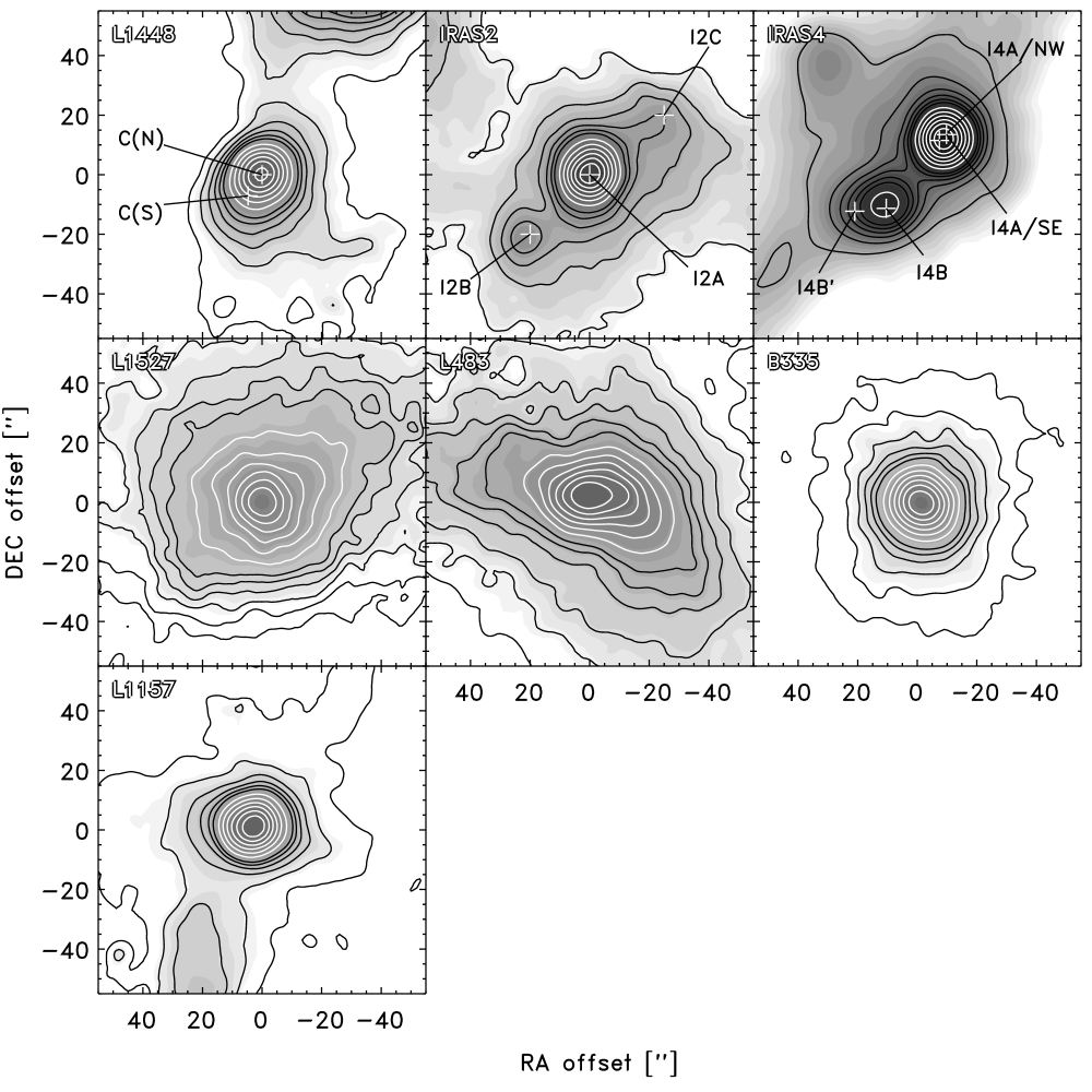
Figure 1: SCUBA maps of the eight sources in our sample from the JCMT archive. In each map the coordinates are given relative to the brightest emission, except in the IRAS4 where a point between the two sources has been chosen as reference. The contour levels are given relative to the peak flux at 5%, 10%, 15%, $\ldots$, 30% (black contours) and from there at 40%, 50%, 60%, $\ldots$, 90% (white contours). In the L1448, IRAS2 and IRAS4 maps, the white plus symbols and labels indicate the individual sources discussed in the text. For further details about the JCMT/SCUBA maps of these regions, see, e.g., Chandler & Richer (2000), Shirley et al. (2000), and Sandell & Knee (2001).

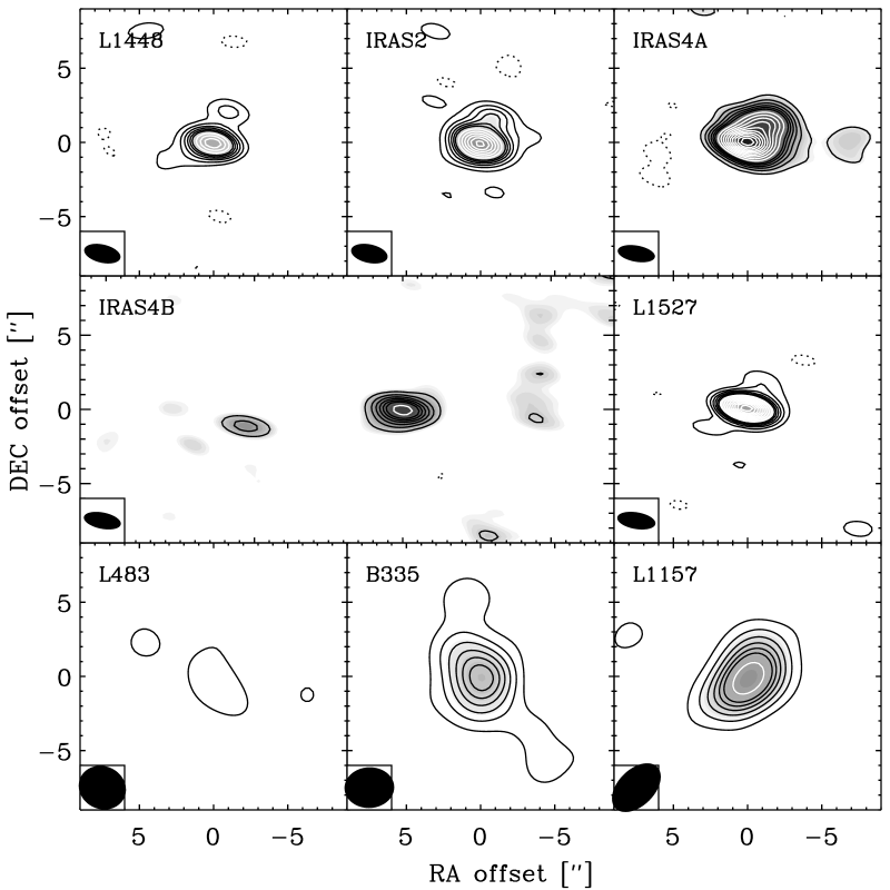
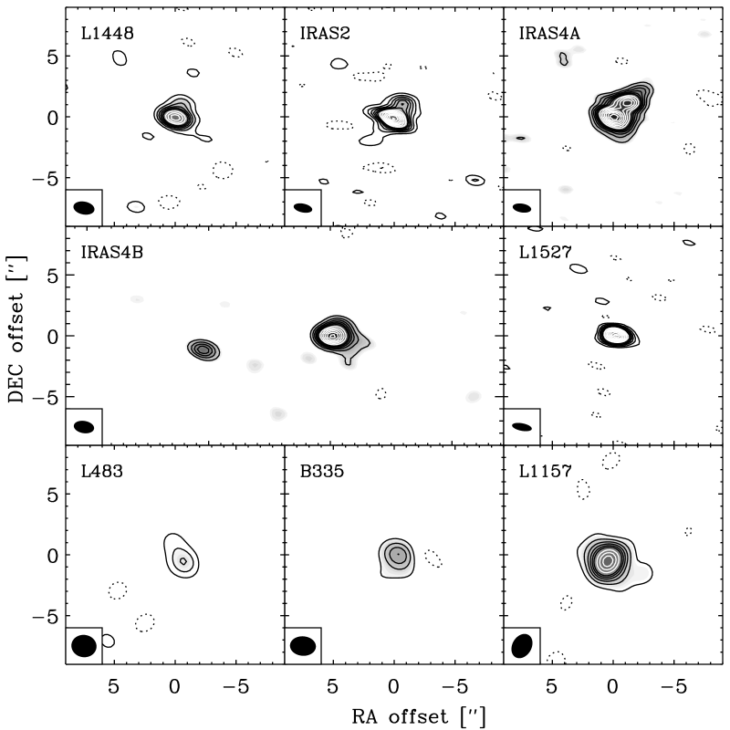
Figure 2: Maps of each of the fields from the 1.3 mm observations (upper panels) and 0.8 mm observations (lower panels) restored with uniform weighting. In each panel, the black contours are given in steps of 3$\sigma$ up to 18$\sigma$ followed by white contours in steps of 6$\sigma$ at 24$\sigma$, 30$\sigma$, 36$\sigma$, $\ldots$. Note that the cores in the lowest row of panels (L483, B335 and L1157) were observed in the compact configuration which gives slightly better sensitivity to extended emission, but lower resolution than the remaining sources observed in the Compact-North configuration.

3.2 Dust continuum emission from protostellar disks

Table 9 and 10 list the derived parameters for each of the bright components from circular Gaussian fits to the visibilities and from point source fits to the longest baselines ($\geq$ 40 k$\lambda$), respectively. The statistical uncertainties on the derived parameters are generally small: the uncertainties on the peak and total fluxes are the largely determined by the RMS noise levels of the data (Table 8) typically 3–5 mJy; somewhat larger, $\approx$10 mJy, for the bright binary sources NGC 1333-IRAS4A and -IRAS4B. On the other hand the calibrational uncertainty on these fluxes is typically 20–30%, therefore dominating the uncertainties on the derived fluxes. Likewise the statistical uncertainties on the positions and sizes of the Gaussians are $\sim 0.1^{\prime\prime}$ or better - largely determined by the S/N of the detections. However, these statistical uncertainties rely on, e.g., the circular Gaussians representing the true distribution of the emission which is likely not to be the case. Therefore, the actual uncertainties on these parameters are larger - but difficult to quantify without more specific models for the distribution of the observed emission.

Comparisons of the total fluxes obtained from the Gaussian fits to the SCUBA maps at 850 $\mu$m (Fig. 1; Chandler & Richer 2000, Shirley et al. 2000 and Sandell & Knee 2001) suggest that typically only 10–20% of the extended emission seen with SCUBA is recovered by the SMA observations. This is also suggested from a comparison between the Gaussian fits at the two frequencies observed with the SMA. Typically the sizes of the Gaussians fit to the 1.3 mm continuum emission are found to be larger than those at 0.8 mm consistent with these sizes reflecting the slightly shorter baselines (in units of k$\lambda$) for the longer wavelength data and thus less resolving out. Also, for a number of the sources, the positions derived for the 230 GHz and 345 GHz continuum observations differ by up to 1″, which is unlikely due to actual differences in the positions but rather reflect the uneven $(u,v)$ sampling. Furthermore, for the sources with the most centrally peaked emission, the best agreement is found between the positions suggesting that the emission from these sources is more weighted to the compact (disk) emission at the center and the envelope mostly resolved out. Fitting the continuum emission with point sources at the longest baselines gives slightly better agreements between the positions from the 0.8 mm and 1.3 mm continuum data. It should be emphasized that some of the sources show variations in fluxes also at longer baselines indicating that the central component is resolved (e.g., IRAS2A Jørgensen et al., 2005a) and for those the fitted point source flux at the given wavelength is an underestimate of the total flux of the compact component.

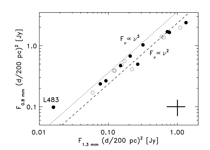
Figure 3: Comparison of the point source fluxes obtained from fits to baselines longer than 40 k$\lambda$. The open symbols show the actual derived fluxes whereas the filled symbols show the fluxes normalized to a distance of 200 pc. The typical calibrational error of $\pm 30$% is indicated in the lower right.

Figure 3 shows a comparison between the 0.8 mm and 1.3 mm continuum fluxes from the point source fits. The point source continuum fluxes at 0.8 mm and 1.3 mm correlate nicely, as expected if they are probing the same unresolved component. It is noteworthy that the continuum flux varies by more than an order of magnitude between the sources at either wavelengths. The only outlier, which does not show a strong detection at the longer baselines, is L483 consistent with the 3 mm observations by Jørgensen (2004).

Interestingly all other sources show compact emission on the longer baselines, which in some cases have been attributed to contributions of central circumstellar disks through models of the observed visibilities (e.g., Keene & Masson, 1990; Hogerheijde et al., 1999; Looney et al., 2003). One problem about such models is the degeneracy between the contributions of disk and envelope emission on small scales and in general it is important to use constraints on the envelope physical structures (such as temperature, density and mass) from other independent observations. A particular powerful method has turned out to be detailed dust radiatve transfer models like those presented for the sources in this sample (Jørgensen et al., 2002). Such models can be used to predict the emission observed by the interferometric observations and address how much the large scale envelope emits on the long baselines/small scales probed by the interferometer and whether an additional component, such as a disk, exists besides this envelope. Four out of the eight sources in this sample have been analysed in this way, specifically: NGC1333-IRAS2A: (Jørgensen et al., 2004b, 2005a); L1448-mm: (Schöier et al., 2004); L483: (Jørgensen, 2004); B335: (Harvey et al., 2003b). These studies typically find that less than $\approx$10–30% of the continuum emission at baselines longer than 40 k$\lambda$ can be attributed to the extended envelope component (see, e.g., Fig. 3 of Jørgensen et al. 2005a). It is therefore as a first approximation reasonable to attribute most of the emission on these longer baselines to a component separate from the envelope.

The strong correlation provides important clues to the nature of these central unresolved sources. For optically thin emission, the slope between the two frequencies, $\alpha$, will be related to the slope, $\beta$, of the dust opacity law, $\kappa\propto\nu^{\beta}$, as $\alpha\approx\beta+2$ in the Rayleigh-Jeans limit (Beckwith & Sargent, 1991). Figure 3 shows that the spectral slopes for all sources are lower than 3.0 with a few lower than 2.0 (average value of 2.4; median 2.6). The optically thin envelope emission would have a spectral slope of 3.5–4 for typical dust opacities which are successfully used to explain the larger scale envelopes in detailed dust radiative transfer models (for example $\beta\approx 1.8$ at 850 $\mu$m for the coagulated dust grains, the so-called “OH5 dust”, of Ossenkopf & Henning (1994) used in Jørgensen et al. (2002)). The protostellar envelopes are not optically thick at 850 $\mu$m - or we should not detect any mid-infrared emission from the central protostars; e.g., Jørgensen et al. (2006). Slopes of 3.5–4 are also what were observed by Dent et al. (1998) in a single-dish survey of the continuum emission from the envelopes around embedded YSOs. We note that since the envelope emission is expected to have a spectral index of 3.5–4, any contribution to the derived point source fluxes will therefore contribute more to the emission at 345 GHz relative to that at 230 GHz compared to the observed flatter spectral indices of 2–3. Thereby subtracting any envelope contribution will in fact flatten the derived spectral index of the compact component.

The flatter spectral indices, $\alpha<3.0$ seen here, suggest that the compact continuum emission has its origin in a different component, likely the disk. Furthermore the spectral indices suggest the compact disk emission is optically thick, and some of the variations in disk fluxes more likely reflect differences in disk sizes and temperatures, rather than mass. For a disk of mass (gas+dust), $M_{D}$ and radius $R_{D}$ the average optical depth is (Beckwith & Sargent, 1991):

$$\langle\tau_{\nu}\rangle=\frac{\kappa_{\nu}/100M_{D}}{\pi R_{D}^{2}\cos\theta}$$ (1)

where $\theta$ is the disk inclination angle and $\kappa_{\nu}$ is the opacity per dust mass (e.g., 1.75 cm² g^-1 at 870 $\mu$m for OH5 dust), which for typical disk parameters (total gas+dust mass of 0.1 $M_{\odot}$ and a radius of 100 AU) can be expressed as:

$$\langle\tau_{870}\rangle=0.5/\cos\theta\left(\frac{M_{D}}{0.1M_{\odot}}\right)\left(\frac{R_{D}}{100{\rm AU}}\right)^{-2}$$ (2)

For example, a lower limit to the disk mass of 0.3 $M_{\odot}$ was derived for NGC1333-IRAS2A from 3 mm observations by Jørgensen et al. (2004b) whereas the disk size was estimated to be 150 AU (radius) in Jørgensen et al. (2005a). This would imply a lower limit to the average optical thickness of about 0.7 at 850 $\mu$m and 0.3 at 1.3 mm (assuming the disk is seen face-on). In terms of its flux, IRAS2A appears typical for the sample of the objects, suggesting that the emission from all the disks in our sample is marginally optically thick. That the emission is marginally optically thick could in fact explain the variations in the derived spectral indices: if any of the highest derived spectral indices had their origin in optically thin emission, the constraint $\alpha<3$ would imply $\beta\lesssim 1$, lower than the $\beta=2$ for typical dust in the interstellar medium. The values of $\alpha\approx 2.0$ would then represent the disks being optically thick. For more evolved T-Tauri and Herbig Ae/Be stars, grain growth has been inferred as an explanation for values of $\beta$ in the range of 0.5–1.0 (e.g., Mannings & Emerson, 1994; Natta et al., 2004; Andrews & Williams, 2005; Draine, 2006; Rodmann et al., 2006; Lommen et al., 2006). Draine (2006) shows that for ISM type dust, $\beta\approx 1$ at 1 mm if the size distribution of the dust grains ($dn/da\propto a^{-p}$ with $p\approx 3.5$) extends to sizes $a_{\rm max}\gtrsim 3$ mm. On the other hand, if the spectral indices are found to be about $2$ all the way to cm wavelengths such as seen in a few objects (IRAS2A, Jørgensen et al. 2005a; L1448-C, Schöier et al. 2004; IRAS16293-2422B Schöier et al. 2004; Chandler et al. 2005), this would imply even larger maximum grain sizes.

If the disks are marginally optically thick, the observed continuum fluxes provide a lower limit to their masses. For optically thin emission from a disk with a single temperature, the disk mass is:

$$M=\frac{S_{\nu}d^{2}}{\kappa_{\nu}B_{\nu}(T)}$$ (3)

or for typical parameters of the dust temperature (30 K) and opacities at 1.3 and 0.8 $\mu$m (Ossenkopf & Henning, 1994):

$$M_{\rm 1.3mm} = 1.3\,M_{\odot}\left(\frac{F_{\rm 1.3~{}mm}}{\rm 1~{}Jy}\right)\left(\frac{d}{\rm 200~{}pc}\right)^{2}\left(\exp\left[0.36\left(\frac{\rm 30~{}K}{T}\right)\right]-1\right)$$ (4)

$$M_{\rm 0.8mm} = 0.18\,M_{\odot}\left(\frac{F_{\rm 0.8~{}mm}}{\rm 1~{}Jy}\right)\left(\frac{d}{\rm 200~{}pc}\right)^{2}\left(\exp\left[0.55\left(\frac{\rm 30~{}K}{T}\right)\right]-1\right)$$ (5)

Using these parameters, Table 10 lists the total masses (gas+dust) of the disks. Given that these disks are likely optically thick rather than thin, the derived masses are lower limits. These disks appear to be at least as massive as typical T-Tauri disks (Andrews & Williams, 2005) (or perhaps more directly; they have comparable fluxes), arguing against a significant build up of the disks from the Class 0 stage to the later T-Tauri stages. Typically the inferred disk masses constitute about 1–10% of the masses of the circumstellar envelopes derived by Jørgensen et al. (2002) (listed in Table 10) and are non-negligible reservoirs of mass. This fraction is also similar to what was found by Looney et al. (2003) who quote compact sources present in their sample of Class 0 sources of 0–0.12 $M_{\odot}$ compared to envelope masses of $\approx 1$ $M_{\odot}$. We emphasize again that these mass estimates are uncertain due to the adopted dust opacities by a factor 2–3 in itself, with additional uncertainties introduced by other parameters such as the disk temperature and exact contribution from the envelope. A detailed comparison to the envelope models and to models for the potential disk structures is required to address these issue, but is outside the scope of this paper.

In summary, the compact continuum emission seen toward the observed protostellar sources likely comes from the circumstellar disks with circumstellar envelopes contributing somewhat at the very shortest baselines. The large number of sources studied homogeneously in this sample allow for direct comparisons between the continuum fluxes and inferred properties of the circumstellar disks. The spectral slopes inferred from the 0.8 mm and 1.3 mm data together with previous longer wavelength observations of a few sources suggest that the emission is marginally optically thick and that the slope of the dust opacity law is $\beta\approx 1$, indicative of grain growth already in the young disks around deeply embedded protostars. The disks are found to contain a significant amount of material with a typical lower limit to the total (gas+dust) mass of about 0.1 $M_{\odot}$ (dependent on assumptions about dust temperatures, opacities etc.), i.e., about 1–10% of the envelope masses. Compared to more evolved T-Tauri stars, the properties of these disks argue against a significant build-up of disks after the deeply embedded stages - or as suggested by Looney et al. (2003), that the processing of material through the disks in the Class 0 stage occur rapidly to avoid a significant build-up of mass. An important aspect of further studies will be to address fully the relative contribution to the continuum emission from the envelope and disks and to model the radial variations of surface densities and optical depth in disks for the sources for which the central continuum component is resolved (e.g., IRAS2A, Jørgensen et al. (2005a)).

Table 9: Results of circular Gaussian fits to the continuum visibilities.

Source	Position			Flux density		Size (FWHM)
	$\alpha$ (0.8 mm)	$\delta$ (0.8 mm)	Offset (1.3 mm)	$F_{\rm 1.3~{}mm}$	$F_{\rm 0.8~{}mm}$	$\theta_{1.3{\rm~{}mm}}$	$\theta_{0.8{\rm~{}mm}}$
	(J2000.0)	(J2000.0)	(arcsec)	[Jy]	[Jy]	[′′]	[′′]
L1448	03 25 38.87	$+$30 44 05.4	($+$0.10 ,$+$0.02)	0.18	0.53	0.94	0.77
IRAS2A	03 28 55.58	$+$31 14 37.1	($+$0.00 ,$+$0.08)	0.34	0.90	1.4	0.94
IRAS4A-SE	03 29 10.54	$+$31 13 30.9	($+$0.08 ,$+$0.09)	1.8	3.5	1.2	1.2
IRAS4A-NW	03 29 10.44	$+$31 13 32.2	($-$0.03 ,$+$0.09)	1.0	2.4	1.2	1.2
IRAS4B	03 29 12.01	$+$31 13 08.1	($+$0.24 ,$-$0.04)	0.92	2.1	1.0	1.0
IRAS4B′	03 29 12.83	$+$31 13 06.9	($+$0.28 ,$-$0.01)	0.25	0.47	0.68	0.63
L1527	04 39 53.88	$+$26 03 09.8	($+$0.26 ,$-$0.01)	0.19	0.58	0.69	0.75
L483	18 17 29.92	$-$04 39 39.5	($+$0.60 ,$-$0.52)	0.044	0.20	3.7	1.7
B335	19 37 00.91	$+$07 34 09.6	($+$0.42 ,$+$0.18)	0.16	0.35	2.9	1.6
L1157	20 39 06.28	$+$68 02 15.8	($-$0.42 ,$+$0.47)	0.30	0.76	2.6	1.7

Table 10: Results of point source fits to the continuum visibilities at baselines longer than 40 k$\lambda$ and mass estimates assuming optical thin dust emission.

Source	Position			Flux density
	$\alpha$ (0.8 mm)	$\delta$ (0.8 mm)	Offset (1.3 mm)	$F_{\rm 1.3mm}$	$F_{\rm 0.8mm}$	$M_{\rm 30K}$	$M_{\rm env}$
	(J2000.0)	(J2000.0)	(arcsec)	[Jy]	[Jy]	[$M_{\odot}$]	[$M_{\odot}$]
L1448	03 25 38.87	$+$30 44 05.4	($+$0.13 ,$-$0.12)	0.12	0.37	0.082 / 0.060	0.93
IRAS2A	03 28 55.58	$+$31 14 37.1	($+$0.05 ,$+$0.01)	0.17	0.48	0.12 / 0.078	1.7
IRAS4A-SE	03 29 10.53	$+$31 13 31.0	($+$0.11 ,$+$0.01)	1.1	2.0	0.76 / 0.32	2.3
IRAS4A-NW	03 29 10.44	$+$31 13 32.3	($+$0.18 ,$-$0.11)	0.59	1.4	0.41 / 0.23	–
IRAS4B	03 29 12.01	$+$31 13 08.1	($+$0.25 ,$-$0.11)	0.59	1.4	0.41 / 0.23	2.0
IRAS4B′	03 29 12.83	$+$31 13 07.0	($+$0.18, $-$0.08)	0.22	0.40	0.15 / 0.065	–
L1527	04 39 53.88	$+$26 03 09.8	($+$0.27 ,$+$0.51)	0.15	0.38	0.072 / 0.025	0.91
L483	18 17 29.91	$-$04 39 39.6	($-$0.18 ,$-$0.48)	0.016	0.097	0.009 / 0.012	4.4
B335	19 37 00.91	$+$07 34 09.7	($-$0.13 ,$+$0.04)	0.059	0.17	0.052 / 0.035	2.6
L1157	20 39 06.28	$+$68 02 16.0	($-$0.38 ,$-$0.01)	0.12	0.39	0.18 / 0.14	1.6

4 Results: Line emission

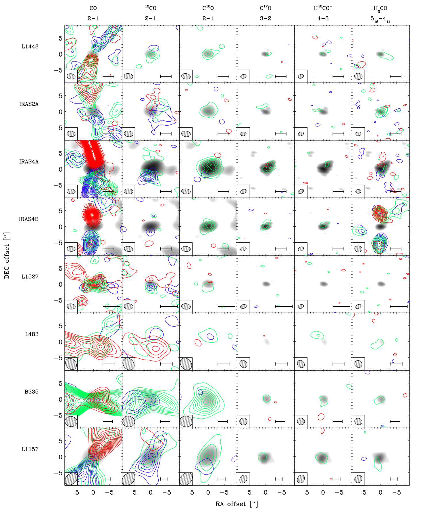
Figure 5: Overview of the entire set of SMA data from the program. Contours given in steps of 3$\sigma$ integrated over the velocity intervals specified in the text (green/blue/red indicate material at the systemic velocity and blue/red shifted from that, respectively). The scale bar in the lower right corner of each panel represents a size of 750 AU toward each source, respectively. The grey scale indicates the continuum emission at 0.8 mm and 1.3 mm (corresponding to the shown line) from Figure 2.

Figure 4 shows the spectra in the central beam toward the continuum peak positions for each detected line while Figure 5 shows maps of the integrated line intensities over three velocity intervals: $[V_{c}-1.5\Delta V;V_{c}-0.5\Delta V]$, $[V_{c}-0.5\Delta V;V_{c}+0.5\Delta V]$ and $[V_{c}+0.5\Delta V;V_{c}+1.5\Delta V]$ around the system velocity $V_{c}$ for each source. $\Delta V$ and $V_{c}$ were chosen based on the widths of Gaussian fitted to the C¹⁸O line at the center positions (Table 11) with $\Delta V=a\,\sigma$ where $\sigma$ is the Gaussian velocity dispersion ($\sigma={\rm FWHM}/(2\sqrt{2\ln(2)}$) and $a=1.5$ for ¹³CO, C¹⁸O 2–1, C¹⁷O 3–2, H¹³CO⁺ 4–3 and C³⁴S 7–6, $a=3$ for SO $5_{6}-4_{5}$, H₂CO $5_{15}-4_{14}$ and CS 7–6, and $a=6$ for CO 2–1, CH₃OH $7_{k}-6_{k}$ and SiO 7–6. Table 12 lists the lines detected toward each source.

Table 11: Result of Gaussian fits to C¹⁸O 2–1 line profiles at the central positions of each source.

Source	$V_{c}$a [km s-1]	FWHMb [km s1]
L1448	5.7	4.3
IRAS2A	7.3	4.3
IRAS4A	6.6	2.7
IRAS4B	7.0	2.0
L1527	5.4	2.0
L483	5.2	2.0
B335	8.5	3.0
L1157	2.9	2.2

^aSystemic velocity: statistical uncertainties from Gaussian fits of 0.05–0.1 km s^-1. ^bLine width (FWHM): statistical uncertainties from Gaussian fits of 0.1–0.3 km s^-1.

All sources show detections in the 2–1 transition of the CO isotopic species at 230 GHz and most sources are detected in the expected strong lines of the main isotopologues of CS 7–6 and H₂CO $5_{15}-4_{14}$ lines at 342.8 and 351.7 GHz, with L1527 being the exception. For the other lines IRAS2A shows strong centrally condensed emission close to the central protostar in all species, whereas the other sources in the sample have detections in only some of the lines with extended emission in some cases.

Table 12: Detected molecular lines.

Line	L1448	IRAS2A	IRAS4A	IRAS4B	L1527	L483	B335	L1157
230 GHz setting
12CO 2–1	+	+	+	+	+	+	+	+
13CO 2–1	+	+	+	+	+	+	+	+
SO $5_{6}-4_{5}$	(O)	+	+	+	+	+*	+	(O)
C18O 2–1	+	+	+	+	+	+	+	+
CH3OH	-	-	-	(O)	-	-	-	-
337 GHz setting
C17O 3–2	(+)	(+)	+	+	-	-	+	+
C34S 7–6	-	+	(+)	-	-	-	-	-
CH3OH $7_{0}-6_{0}$	(+)	+	O	O	-	+	-	-
CH3OH $7_{-1}-6_{-1}$	(+)	+	O	O	-	+	-	-
CH3OH $7_{\pm 2}-6_{\pm 2}$	-	+	O	O	-	-	-	-
CH3OH $7_{k}-6_{k}$	-	+	-	-	-	-	-	-
SiO 8–7	-	-	(O)	O	-	-	-	-
HN13C 4–3	-	-	-	-	-	-	-	-
H13CO+ 4–3	+	-	-	+*	-	+*	-	+
342 GHz setting:
CS 7–6	+	+	+/O	+/O	-	+	+	+
H2CO $5_{15}-4_{14}$	+	+	+/O	O	-	(+)	+	+
SO2	(+)	-	-	-	-	-	-	-

Note. — Units of right ascension are hours, minutes, and seconds and units of declination are degrees, arcminutes and arcseconds. See the text for a discussion of the uncertainties of the derived parameters.

Note. — Units of right ascension are hours, minutes, and seconds and units of declination are degrees, arcminutes and arcseconds. See the text for a discussion of the uncertainties of the derived parameters.

Note. — “+” indicates that line emission detected above 3$\sigma$ toward the central source position, “O” that the line is detected in the outflow offset from the central protostar, “*” that line emission is detected offset from the central protostar and also not obviously connected to any outflow shocks and “-” that no emission is detected. Symbols given in parenthesis indicate tentative detections.

As with the continuum observations, a significant fraction of the line emission is resolved out - and only the brightest, most compact regions are detected. For most species and sources, this occurs close to the continuum positions - as one would expect from a centrally condensed envelope. It is also seen that the sources which are observed with the shortest possible baselines in the Compact configuration show stronger emission in some of the prominent lines: for example, strong C¹⁷O 3–2 emission is detected in L1157 whereas it does not show particularly strong C¹⁷O 3–2 lines compared to the other sources in the survey of Jørgensen et al. (2002). Again, this likely reflects that most of the C¹⁷O 3–2 emission seen in the single-dish observations comes from the extended envelope and thus is very sensitive to the differences in the lengths of the shortest baselines.

The amount of resolving out for a somewhat extended molecular species is estimated by comparison to the single-dish observations of C¹⁸O 2–1 by Jørgensen et al. (2002) (for B335, CSO observations presented by Evans et al. (2005) were used). The integrated line intensities from the single-dish observations are converted from antenna temperature scales to Jy beam^-1 using the standard expressions and compared to the central spectra from either the interferometer datasets restored with a beam size comparable to the single-dish beam size (in cases where the signal-to-noise is sufficient) or the flux integrated over a smaller region where the emission was detected. For C¹⁸O 2–1 the amount of flux recovered by the interferometer estimated in this way varies from 1–3% for L1448, IRAS2A, IRAS4B, L1527 and L483, about 6% for IRAS4A to 16% and 22% for L1157 and B335, respectively. The slightly higher amount of recovered emission in IRAS4A (compared to the other sources observed in the Compact-North configuration) and vice versa the slightly lower amount of recovered emission in L483 (compared to the sources observed in the compact configuration) are nice examples of the importance of source structure. IRAS4A has significant structure within the single-dish beam, in particular by the two binary components well separated by the interferometer and each contributing to the total flux, whereas L483 typically shows a more smooth distribution of its emission over larger scales. Still, since only 15–20% of the emission is recovered even in the best cases of B335 and L1157, it is clear that care must be taken when interpreting the interferometric data. It is, for example, not possible to deduce quantitative information from the integrated line fluxes without compensating for the lack of short spacing data.

Two sources, IRAS4A and IRAS4B, show characteristic “inverse P Cygni” line profiles where the red-shifted part of the lines is seen in absorption against the continuum while the blue-shifted part is seen in emission. Such profiles can be taken as the least ambiguous evidence for infall in protostellar cores where the foreground material falling toward the central source (red-shifted) is absorbing the continuum emission. Inverse P Cygni profiles have been seen previously in lines of H₂CO and CS toward IRAS4A and IRAS4B in IRAM Plateau de Bure observations by Di Francesco et al. (2001). With the SMA operating at submillimeter wavelengths (and therefore measuring stronger continuum emission and high excitation lines), it should be ideally suited for detecting such line profiles. Of all the lines in the sample, only the ¹³CO 2–1 lines toward IRAS4A and IRAS4B show clear inverse P Cygni profiles (Figure 6). Together with IRAS 16293-2422 (Chandler et al., 2005; Takakuwa et al., 2006a; Remijan & Hollis, 2006), these sources provide the only known examples of inverse P Cygni profiles toward low-mass protostars. It could suggest that the observed inverse P Cygni profiles are related to much larger scale infalling motions such as those seen in single-dish observations of IRAS4 by Walsh et al. (2006) rather than collapse onto the central protostar. The 230 GHz continuum emission toward IRAS4A is marginally resolved between the two components of the binary and no significant difference is seen between the widths of the absorption across the continuum possibly arguing in favor of the presence of more global collapsing motions.

Figure 4: Spectra toward the center position of each source.

Figure 6: ¹³CO 2–1 spectra toward the center positions of IRAS2A, IRAS4A and IRAS4B.

4.1 Dynamical impact of outflows

Of all the lines in the survey, the CO 2–1 lines provide the most striking features, showing extended outflow emission over most of the SMA primary beam (Figure 7). The CO emission has significant differences, from the highly collimated IRAS4B outflow to the somewhat more diffuse L483, L1527 and B335 outflows. The close binarity of IRAS2A and IRAS4A is also seen in the CO maps causing more confusing pictures of those outflows. IRAS2A for example shows hints of both a prominent north-south cone-shaped outflow and a more collimated east-west jet (see also discussion in Jørgensen et al., 2004a, b). For L1448, IRAS2A and L1157, the CO emission is seen to delineate the edges of the outflow cavities.

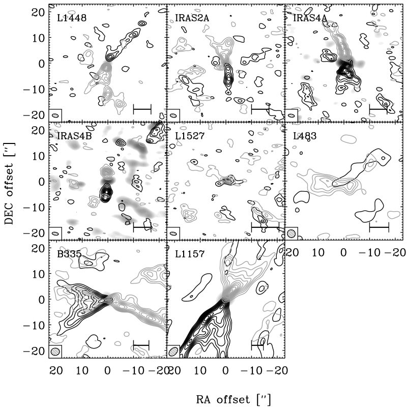
Figure 7: Map of the CO 2–1 emission over the entire interferometer field of view for each source in the sample. The contours are shown in steps of 3$\sigma$ with the black contours indicating emission integrated from $-$6 km s^-1 to $-$1 km s^-1 relative to the systemic velocity and grey contours emission integrated from +1 km s^-1 to +6 km s^-1 relative to the systemic velocity. The scale bar in the lower right corner of each plot indicates a length of 1500 AU at the distance of the respective source.

It should be emphasized that some of the differences between outflows in this sample could be due to inclination effects. A highly collimated outflow directed in the plane of the sky will have small relative CO velocities over the extent of the outflow and its CO emission will be more susceptible to resolving out as it merges with the surrounding cloud material. L1527 shows a “butterfly” shape in lower-$J$ CO and HCO⁺ lines (Tamura et al., 1996; Hogerheijde et al., 1997), suggesting that inclination is significant there. Likewise, an outflow with a large opening angle viewed at an inclination close to the opening of the outflow cones will show both red- and blue-shifted emission overlapping in both lobes, which has been shown to be the case for B335 (Cabrit et al., 1988).

Recently, Arce & Sargent (2006) imaged a sample of nine Class 0, I and II young stellar objects in the ¹²CO 1-0 line observed with the Owens Valley Radio Observatory Millimeter Array. They found that outflow opening angles are a good discriminant between the different evolutionary stages of the objects and suggested that it reflects that the material in the protostellar envelope is cleared as the outflow opens up an increasingly wide cavity. A similar suggestion has been put forward by Velusamy & Langer (1998).

All of the outflows in our sample are found to have small opening angles ($\lesssim 60^{\circ}$), further supporting the conclusion of Arce & Sargent that the outflows with the narrowest opening angles belong to the Class 0 objects. The individual outflows in our sample share many of the features with the three different Class 0 outflows in the sample of Arce & Sargent, ranging from the jet-like IRAS4B, IRAS4A2 and IRAS2A (east-west) outflows (similar to the HH114-mms outflow from the sample of Arce & Sargent), to the more cone-like L1448, IRAS2A (north-south), B335 and L1157 outflows (similar to the IRAS 03282+3035 outflow in the Arce & Sargent sample). In addition the diffuse L483 and L1527 outflows appear more similar to the Class I outflows in the sample of Arce & Sargent. It is interesting to note that no significant changes in the shape of the cone is seen for the observed outflows all the way to the few hundred AU scales probed by the SMA observations, in contrast with what is expected if the outflow angle increases over the duration of the Class 0 stage. That is, the outflows do not show a parabolic shape reflecting a larger opening angle close to the central protostar compared to material further away - in contrast to what is seen in the perhaps best example of this scenario in B5-IRS1 (Velusamy & Langer, 1998).

It is also interesting to note that the most collimated outflows (IRAS4A and IRAS4B) are related to the objects with the highest ratios of disk to envelope masses from the continuum studies while the objects with the lowest disk masses compared to envelope masses (L1527 and L483) show the most diffuse outflows. This may seem a disparity; in a simple picture of envelope material falling into a circumstellar disk and accreting onto the central protostar, the mass of the disk is expected to increase until the envelope has dissipated (e.g., Nakamoto & Nakagawa, 1994; Hueso & Guillot, 2005). One would therefore expect that the more evolved (still embedded) objects would have the highest disk-to-envelope mass ratios in contrast to what is observed here.

The question is whether L483 and L1527 still will accrete significant material from the currently observed dust envelope. As pointed out in §3.1, both show very flat density profiles from the SCUBA maps, which could reflect the importance of heating of the protostellar envelopes through their outflow cavities. Indeed, both sources show near-infrared scattering nebulosities (e.g., Tamura et al., 1991; Fuller et al., 1995; Jørgensen, 2004), supporting the view that their envelopes are being heated at larger scales. The high angular resolution N₂H⁺ observations of L483 by Jørgensen (2004) furthermore indicate a velocity gradient in the larger scale quiescent envelope material in the direction of the outflow, likely reflecting that the envelope indeed is being dispersed by the action of the outflow. It is therefore plausible that L1527 and L483 in particular, are in a phase where the accretion has more or less come to a stop - and the protostar just is “waiting” to disperse its remaining envelope through the action of the outflow. The relatively large disk masses of the remaining objects could imply that they also are close to the maximum disk masses - but comparisons to both disk and envelope structures of more evolved Class I objects are needed to confirm or refute this. Also, firmer constraints on both disk structures and outflow parameters for these sources will be important to obtain a more quantitative picture of the dynamical properties of the envelope and disk material.

4.2 Chemical impact of outflows

Another example of the importance of the outflows is most clearly seen in the chemical differentiation toward some of the sources. For IRAS4B, for example, a number of lines show emission separated into clumps about 6″ (1500 AU) north/south of the central protostar, prominently seen in CS, CH₃OH and H₂CO. These species are found to be located on the tips of the CO outflows and likely probe shocks where the outflow impacts the envelope. In IRAS4A, characteristic shocks (although less prominent than in IRAS4B) are seen north and south in the outflow associated with the northwestern binary component, IRAS4A-NW (IRAS4A2). Fainter compact emission is also seen toward the center of this source; interestingly, this emission appears to be red-shifted with respect to the systemic velocity, also suggesting an outflow impact on the smallest scales. The shock-tracing SiO and SO emission also peak away from the central protostars in IRAS4A and IRAS4B, although only a very tentative SiO emission is observed toward IRAS4A. For three other sources in the sample, compact CH₃OH emission is seen, most prominently in IRAS2A. In contrast to the two other sources in NGC 1333, a number of high excitation transitions are observed in the CH₃OH $7_{k}-6_{k}$ band toward this source. This is indicative of the presence of hot gas on small scales in IRAS2A, consistent with the conclusion of Jørgensen et al. (2005a) who imaged even higher excitation CH₃OH transitions also with the SMA.

The three sources in NGC 1333 (IRAS2A, IRAS4A and IRAS4B) have all been suggested to have “hot corinos” (e.g. Maret et al., 2004), i.e., inner regions where the temperature increases above 100 K due to passive heating by the protostar and where complex organic molecules are produced into the gas-phase as ice mantles evaporate. This was in particular inferred from multi-transition observations of H₂CO and CH₃OH which in some cases could not be fit by constant abundances. Maret et al. (2004, 2005) discussed these single-dish observations in context of the hot corino scenario and found that these sources required an abundance enhancement by up to four orders of magnitude in the innermost regions. Jørgensen et al. (2005b) on the other hand demonstrated that those abundance enhancements in most cases were a result of specific assumptions, e.g., about the ratio between the abundances ortho- and para-H₂CO. Furthermore, shocks caused by the outflows can enhance the abundances of these species on larger scales which further complicates the interpretation of hot corinos: Jørgensen et al. (2005b), for example, found that the H₂CO and CH₃OH abundance variations in IRAS4B were best explained by a scenario in which the molecules were released in the outflow driven shocks, further supported by the line profiles of these species and high excitation CS 10–9 lines.

To properly address these issues high angular resolution observations are clearly important, e.g., to directly image where molecular species have their origin. Mundy et al. (1992) for example demonstrated that the emission of SO toward the inner few arcseconds of the Class 0 source IRAS 16293-2422 was enhanced by the action of the outflow also traced by centimeter continuum emission and H₂O maser activity. More recently, Bottinelli et al. (2004) resolved the emission of complex organic species, CH₃CN and HCOOCH₃, toward this source and derived a size of $\sim 100$ AU, comparable to the expected size of the hot corino. Chandler et al. (2005) on the other hand found that the emission of high excitation transitions and complex organic molecules toward this source was shifted by a few tenths of an arcsecond ($\sim 50$ AU) coinciding with the shock seen in longer wavelength continuum observations. The SMA observations presented in this paper indicates that the peaks in the CH₃OH and H₂CO emission toward IRAS4A-NW and IRAS4B are related to the shocks and that no trace of compact emission from these species is seen toward the central continuum sources, in contrast to what should be expected in the case of hot corinos. We note that also for these transitions the SMA resolve out a significant fraction (50–75%) of the observed single-dish flux indicating that H₂CO and CH₃OH are present in the large scale envelopes.

IRAS2A still stands out with compact hot gas as witnessed, e.g., by the detection of many of the higher excitation hyperfine components of the $J=7-6$ line (Fig. 9 and higher $J$ CH₃OH lines (Jørgensen et al., 2005a) that appear unresolved. Of the well-studied low-mass protostars, IRAS2 therefore appears to be the best hot corino candidate. Given the importance of outflows in the other low-mass sources where complex organic molecules have been observed, however, it is a valid question to ask whether the protostellar outflow is important on these small scales in IRAS2A, where it is still unresolved by the SMA observations (similar to the case of IRAS 16293-2422). The SO emission do show evidence of a velocity gradient which could suggest that the shocks are impacting the material on small scales toward IRAS2A. Also, it is possible that accretion shocks in the disk could temporarily heat the gas in the surface layer to high temperatures and likewise inject complex molecules from the ice mantles into the gas-phase. In IRAS2A in particular, this seems to be a feasible scenario, given the extent of the disk from submillimeter continuum data (see discussion in Jørgensen et al., 2005a). Again, further high-resolution line observations could potentially disentangle the velocity field of the disk and further address its physical properties (temperature, density) and chemical structure.

This discussion directly illustrates the importance of high-angular resolution imaging for the interpretation of chemical variations in protostellar environments. With the high-resolution SMA observations, it becomes possible to image directly these physical and chemical variations in the immediate vicinity of the low-mass protostars.

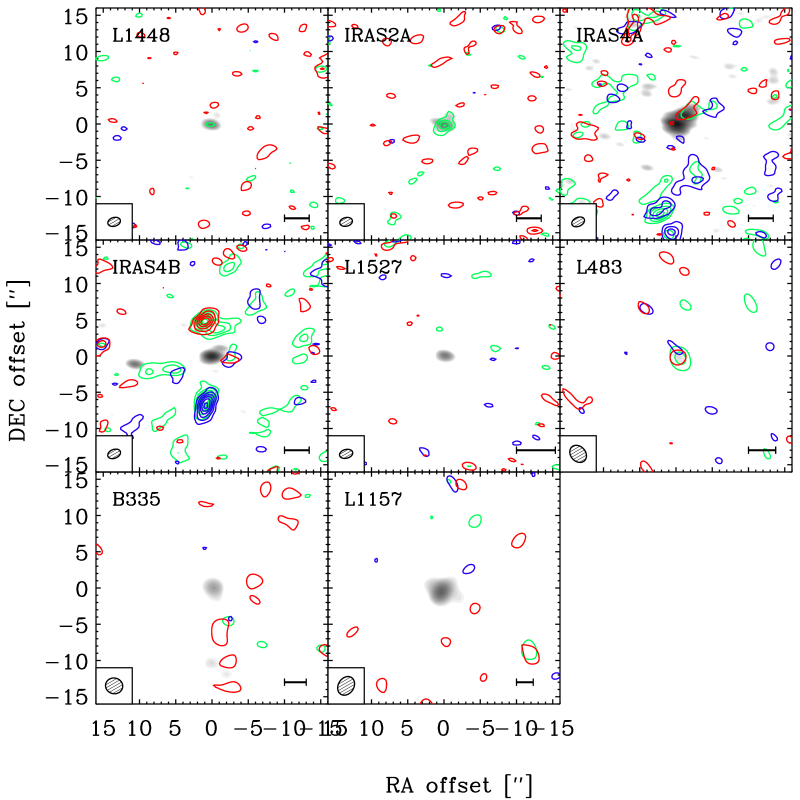
Figure 8: CH₃OH $7_{0}-6_{0}$ and $7_{-1}-6_{-1}$ emission (added-up) toward the entire sample of sources. The emission has been integrated over the same velocity intervals as in Fig. 5. The scalebar in the lower right corner of each plot indicates a scale of 750 AU at the distance of each source.

Figure 9: Higher excitation CH₃OH $7_{k}-6_{k}$ transitions toward the center positions of IRAS2A, IRAS4A and IRAS4B. The location of the transitions have been marked with vertical lines, from left through right: 0A (also shown in Figure 8), -6E, 6A, -5E, 5E, 5A and -4E.

5 Summary

A large line and continuum survey with the Submillimeter Array of 8 deeply embedded, low-mass protostellar cores has been presented. Each source has been observed in three different spectral settings that included lines of the most common molecular species, CO, HCO⁺, CS, SO, H₂CO, CH₃OH and SiO. Emission from (sub)millimeter lines from 11 molecular species (including isotopologues) have been imaged at high angular resolution (1^′′–3^′′; typically corresponding to 200–600 AU) together with continuum emission at 230 (1.3 mm) and 345 GHz (0.8 mm). A number of conclusions can be inferred from simple considerations of this dataset:

• Compact continuum emission is observed for all sources. Comparing the 230 GHz and 345 GHz data, the emission is found to be well described as $F\propto\nu^{\alpha}$ with an average value of $\alpha$ of 2.4. $\alpha>3.0$ was only found for one source, L483. For this source, the compact continuum emission is weak at 230 GHz and the emission comes from the envelope rather than the circumstellar disk. For the remaining sources, the continuum emission likely originates in the disks being marginally optically thick and having dust opacities, $\kappa_{\nu}\propto\nu^{\beta}$ with $\beta\approx 1$. Lower limits to the total disk masses (gas+dust) are found to be typically 0.1 $M_{\odot}$ for a dust temperature of 30 K (1–10% of their envelope masses).

• Inverse P Cygni profiles indicative of infalling motions are seen in the ¹³CO 2–1 lines toward IRAS4A and IRAS4B. These are not observed in other lines or toward other sources (besides IRAS 16293-2422), however, and it is possible that these profiles have their origin in the ambient cloud/outer envelope rather than infall in the inner envelope themselves.

• Prominent outflows are present in all sources extending over most of the interferometer field of view. Most of the outflows show small opening angles $\lesssim 60^{\circ}$ comparable to other previously studied Class 0 objects - and in agreement with the suggestion that the outflow opening angle increases with time (Velusamy & Langer, 1998; Arce & Sargent, 2006). Still, significant differences are seen in their morphologies with some outflows showing more jet-like structure and others seemingly tracing material in the outflow cavity walls. The most diffuse outflows are found for the objects with the lowest ratios of disk-to-envelope masses, in particular L1527 and L483, which are thought to be transitionary between the Class 0 and I stages. It is suggested that these sources have reached the end of their main accretion and that the remaining envelope material will be dispersed by the outflows.

• Shocks are present on all scales in the protostellar environments, most clearly traced by extended emission of CH₃OH in IRAS4A and IRAS4B. Compact red-shifted CH₃OH emission is seen toward one of the components of the IRAS4A binary, IRAS4A-NW (IRAS4A2). These observations suggest that the emission of H₂CO and CH₃OH, often taken as signposts of low-mass “hot corinos”, are in fact related to the shocks caused by the protostellar outflows. In this context, IRAS2A stands out as the only source with clear evidence for hot, compact gas (as also seen in previous SMA observations by Jørgensen et al. 2005a). Further high resolution observations will be necessary to ascertain whether this emission is related to a passively heated hot corino, a shock in the circumstellar disk or perhaps just the action of the outflow on the smallest scales.

It is clear that these high-resolution observations pushes our understanding of embedded protostars as simple and quiescent structures toward a more dynamic picture. Outflows play an important role in all aspects of the structure of these low-mass protostellar systems, from the larger scale swept up material clearly probed by the CO outflows down to the smallest (arcsecond) scales where shocks are present. It is important to realize that the larger scale envelope carrying the bulk of the material probed by single-dish observations is almost completely resolved out by the SMA observations. Using the SMA data in conjunction with single-dish data and/or detailed models for the source structures, it will become possible to make quantitative statements, e.g., about the physical structure of the envelopes or the chemical abundances from scales of thousands of AU down to just the few hundred AU probed by the interferometers. More detailed discussions of aspects of star formation based on the data presented in this paper, in addition to such single-dish data and detailed radiative transfer models, will be presented in a series of upcoming specialized papers.

Appendix A Description of sources

A.1 L1448-C(N)

L1448-C(N) is one of $\sim$10 young stellar objects in the L1448 complex in the Perseus molecular cloud. Recent Spitzer observations (Jørgensen et al., 2006) have resolved it into two components with a separation of about 8″ (2000 AU). The northern of these two is known from millimeter aperture synthesis observations (e.g., Barsony et al., 1998; Schöier et al., 2004) which is taken as the pointing center for the observations in this paper.

A.2 NGC 1333-IRAS2A

NGC 1333-IRAS2A is part of a protostellar system also encompassing the protostar IRAS2B and likely pre-stellar core IRAS2C seen in SCUBA maps (Sandell & Knee, 2001). Both IRAS2A and IRAS2B have been imaged at high angular resolution at millimeter wavelengths (Blake, 1996; Looney et al., 2000; Jørgensen et al., 2004b) whereas IRAS2C does not show any compact continuum emission. IRAS2B is located outside the primary beam field of view at a separation of 30^′′ (7500 AU), but is detected in the 1.3 mm maps presented here. IRAS2A itself has been speculated to be a protostellar binary, resulting in its characteristic quadrupolar outflow (see also §4.1). At 0.8 mm, it appears to be resolved into two separate components with a fainter companion northeast of the main peak, but as for L1448 above, it is not clear whether this is simply a result of resolving out differing amounts of envelope material. Jørgensen et al. (2005a) examined SMA continuum observations from IRAS2A and showed that the emission could be explained by a combination of an extended envelope and a 300 AU diameter disk.

A.3 NGC 1333-IRAS4A

NGC 1333-IRAS4A (together with its companion IRAS4B; both well-separated in SCUBA maps) is one of the most well-studied protostellar systems in NGC 1333. Di Francesco et al. (2001) detected inverse P Cygni profiles indicative of infalling motions in lines of H₂CO toward these sources. IRAS4A is resolved into two binary components, NGC 1333-IRAS4A-NW and -IRAS4A-SE with a separation of 1.8^′′ (400 AU) (Lay et al., 1995; Looney et al., 2000; Di Francesco et al., 2001).

A.4 NGC 1333-IRAS4B

NGC 1333-IRAS4B is located about 30″ southeast of NGC 1333-IRAS4A and also shows signs of inverse P Cygni profiles (Di Francesco et al., 2001). A fainter companion NGC 1333-IRAS4B^′ (also sometimes referred to as NGC 1333-IRAS4C or NGC 1333-IRAS4B2) is located another 10″ to the east (Looney et al., 2000; Di Francesco et al., 2001). The outflow in IRAS4B appears to play an important role of 5–10″ scales affecting the emission of a number of molecular species. Jørgensen et al. (2005b) for example found that the abundance variations of H₂CO and CH₃OH deduced from single-dish observations best were explained by the impact of this outflow - also accounting for the line profiles of these species and high excitation CS 10–9 emission detected toward this source.

A.5 L1527-IRS

L1527-IRS (IRAS 04368+2557) is one of the possibly more evolved protostars in the sample located in a dense core in Taurus. L1527-IRS was previously studied at high angular resolution with the Nobeyama Millimeter Array (Ohashi et al., 1997) and the Owens Valley Radio Observatory Millimeter Array (OVRO; Hogerheijde et al., 1997, 1998) and found to show a characteristic X-shaped structure in lines of ¹³CO 1–0 and HCO⁺ that likely delineates the walls of an outflow cavity. It was suggested to be a binary based on 800 $\mu$m continuum observations (Fuller et al., 1996) with the secondary at about 21″ from the main protostar. No evidence is found of this secondary in the previous high resolution 3 mm maps or in the maps presented here, however (it would be located outside the primary beam field of view at 345 GHz, but inside at 230 GHz). The SCUBA maps show a very extended core with little central concentration (a flat envelope density profile $n\propto r^{-p}$ with $p=0.6-1.0$ is found for this source (Jørgensen et al., 2002; Shirley et al., 2002) whereas most of the other protostars have steeper profiles with $p=1.5-2.0$).

A.6 L483-mm

L483-mm is a strong infrared source (IRAS 18148-0440) associated with an isolated core. Tafalla et al. (2000) suggested it was transitionary between the Class 0 and I stages. It has been imaged at high resolution in continuum and lines at 3 mm with the Berkeley Maryland Illinois Association (BIMA) Millimeter Array (Park et al., 2000) and OVRO MMA (Jørgensen, 2004). In the analysis of the continuum emission Jørgensen (2004) found that all the detected continuum emission could be attributed to the extended envelope, contrasting L483-FIR from L1448-C and NGC 1333-IRAS2A described above where a compact continuum source was present. Takakuwa et al. (2006b) recently mapped L483-mm in the HCN 4–3 transition at submillimeter wavelengths using the ASTE single-dish telescope. They found that the HCN emission was slightly extended, which they argued is reflecting the heating of the envelope material to 4000 AU scales through the outflow cavity.

A.7 B335

B335 has often been considered one of the best protostellar collapse candidates. It has been imaged in continuum at subarcsecond resolution (Harvey et al., 2003b, a) and in lines (Wilner et al., 2000). Harvey et al. (2003a) found that the continuum emission could be well described by a $n\propto r^{-1.5}$ envelope down to scales of $\sim 100$ AU within which a disk with a size $\lesssim$ 100 AU is seen. Wilner et al. (2000) showed that the line emission thought to trace the collapse were in fact dominated by a number of clumps extending along the outflow cavity into the low density medium.

A.8 L1157-mm

L1157-mm is perhaps best known for its prominent outflow (Bachiller & Pérez Gutiérrez, 1997; Bachiller et al., 2001), but also its small-scale envelope/disk structure has gotten a fair amount of attention. Gueth et al. (1997) observed L1157 in lines of CO (and isotopologues) and continuum using the IRAM Plateau de Bure interferometer (PdBI). They found that the continuum emission probed a combination of a large disk and an extended envelope with a clear outflow cavity whereas the CO isotopologues probed a progression from the envelope, throughout its cavities to the outflow itself. Goldsmith et al. (1999) and Velusamy et al. (2002) observed transitions of CH₃OH at 3 mm and 1.3 mm using OVRO, suggesting that these CH₃OH transitions had their origin in a warm layer of the disk heated by an accretion shock.

References

- André et al. (1993) André, P., Ward-Thompson, D., & Barsony, M. 1993, ApJ, 406, 122
- André et al. (2000) André, P., Ward-Thompson, D., & Barsony, M. 2000, in Protostars and Planets IV, ed. V. Mannings, A. P. Boss, & S. S. Russell (University of Arizona Press, Tucson), 59
- Andrews & Williams (2005) Andrews, S. M., & Williams, J. P. 2005, ApJ, 631, 1134
- Arce & Sargent (2006) Arce, H. G., & Sargent, A. I. 2006, ApJ, 646, 1070
- Bachiller et al. (2001) Bachiller, R., Pérez Gutiérrez, M., Kumar, M. S. N., & Tafalla, M. 2001, A&A, 372, 899
- Bachiller & Pérez Gutiérrez (1997) Bachiller, R., & Pérez Gutiérrez, M. 1997, ApJ, 487, L93
- Barsony et al. (1998) Barsony, M., Ward-Thompson, D., André, P., & O’Linger, J. 1998, ApJ, 509, 733
- Beckwith & Sargent (1991) Beckwith, S. V. W., & Sargent, A. I. 1991, ApJ, 381, 250
- Blake (1996) Blake, G. A. 1996, in IAU Symp. 178: Molecules in Astrophysics: Probes & Processes, ed. E.F. van Dishoeck (Kluwer Academic Publishers, Dordrecht)
- Bottinelli et al. (2004) Bottinelli, S., et al. 2004, ApJ, 617, L69
- Cabrit et al. (1988) Cabrit, S., Goldsmith, P. F., & Snell, R. L. 1988, ApJ, 334, 196
- Chandler et al. (2005) Chandler, C. J., Brogan, C. L., Shirley, Y. L., & Loinard, L. 2005, ApJ, 632, 371
- Chandler & Richer (2000) Chandler, C. J., & Richer, J. S. 2000, ApJ, 530, 851
- Dent et al. (1998) Dent, W. R. F., Matthews, H. E., & Ward-Thompson, D. 1998, MNRAS, 301, 1049
- Di Francesco et al. (2001) Di Francesco, J., Myers, P. C., Wilner, D. J., Ohashi, N., & Mardones, D. 2001, ApJ, 562, 770
- Draine (2006) Draine, B. T. 2006, ApJ, 636, 1114
- Evans et al. (2005) Evans, N. J., Lee, J.-E., Rawlings, J. M. C., & Choi, M. 2005, ApJ, 626, 919
- Fuller et al. (1995) Fuller, G. A., Lada, E. A., Masson, C. R., & Myers, P. C. 1995, ApJ, 453, 754
- Fuller et al. (1996) Fuller, G. A., Ladd, E. F., & Hodapp, K.-W. 1996, ApJ, 463, L97
- Goldsmith et al. (1999) Goldsmith, P. F., Langer, W. D., & Velusamy, T. 1999, ApJ, 519, L173
- Gueth et al. (1997) Gueth, F., Guilloteau, S., Dutrey, A., & Bachiller, R. 1997, A&A, 323, 943
- Harvey et al. (2001) Harvey, D. W. A., Wilner, D. J., Lada, C. J., Myers, P. C., Alves, J. F., & Chen, H. 2001, ApJ, 563, 903
- Harvey et al. (2003a) Harvey, D. W. A., Wilner, D. J., Myers, P. C., & Tafalla, M. 2003a, ApJ, 596, 383
- Harvey et al. (2003b) Harvey, D. W. A., Wilner, D. J., Myers, P. C., Tafalla, M., & Mardones, D. 2003b, ApJ, 583, 809
- Ho et al. (2004) Ho, P. T. P., Moran, J. M., & Lo, K. Y. 2004, ApJ, 616, L1
- Hogerheijde et al. (1997) Hogerheijde, M. R., van Dishoeck, E. F., Blake, G. A., & van Langevelde, H. J. 1997, ApJ, 489, 293
- Hogerheijde et al. (1998) Hogerheijde, M. R., van Dishoeck, E. F., Blake, G. A., & van Langevelde, H. J. 1998, ApJ, 502, 315
- Hogerheijde et al. (1999) Hogerheijde, M. R., van Dishoeck, E. F., Salverda, J. M., & Blake, G. A. 1999, ApJ, 513, 350
- Huard et al. (1999) Huard, T. L., Sandell, G., & Weintraub, D. A. 1999, ApJ, 526, 833
- Hueso & Guillot (2005) Hueso, R., & Guillot, T. 2005, A&A, 442, 703
- Jørgensen (2004) Jørgensen, J. K. 2004, A&A, 424, 589
- Jørgensen et al. (2005a) Jørgensen, J. K., Bourke, T. L., Myers, P. C., Schöier, F. L., van Dishoeck, E. F., & Wilner, D. J. 2005a, ApJ, 632, 973
- Jørgensen et al. (2006) Jørgensen, J. K., et al. 2006, ApJ, 645, 1246
- Jørgensen et al. (2004a) Jørgensen, J. K., Hogerheijde, M. R., Blake, G. A., van Dishoeck, E. F., Mundy, L. G., & Schöier, F. L. 2004a, A&A, 415, 1021
- Jørgensen et al. (2004b) Jørgensen, J. K., Hogerheijde, M. R., van Dishoeck, E. F., Blake, G. A., & Schöier, F. L. 2004b, A&A, 413, 993
- Jørgensen et al. (2002) Jørgensen, J. K., Schöier, F. L., & van Dishoeck, E. F. 2002, A&A, 389, 908
- Jørgensen et al. (2004) Jørgensen, J. K., Schöier, F. L., & van Dishoeck, E. F. 2004, A&A, 416, 603
- Jørgensen et al. (2005b) Jørgensen, J. K., Schöier, F. L., & van Dishoeck, E. F. 2005b, A&A, 437, 501
- Keene & Masson (1990) Keene, J., & Masson, C. R. 1990, ApJ, 355, 635
- Kuan et al. (2004) Kuan, Y., et al. 2004, ApJ, 616, L27
- Lay et al. (1995) Lay, O. P., Carlstrom, J. E., & Hills, R. E. 1995, ApJ, 452, L73
- Lee et al. (2006) Lee, C.-F., Ho, P. T. P., Beuther, H., Bourke, T. L., Zhang, Q., Hirano, N., & Shang, H. 2006, ApJ, 639, 292
- Lommen et al. (2006) Lommen, D., et al. 2006, A&A, in press.
- Looney et al. (2000) Looney, L. W., Mundy, L. G., & Welch, W. J. 2000, ApJ, 529, 477
- Looney et al. (2003) Looney, L. W., Mundy, L. G., & Welch, W. J. 2003, ApJ, 592, 255
- Mannings & Emerson (1994) Mannings, V., & Emerson, J. P. 1994, MNRAS, 267, 361
- Maret et al. (2004) Maret, S., et al. 2004, A&A, 416, 577
- Maret et al. (2005) Maret, S., Ceccarelli, C., Tielens, A. G. G. M., Caux, E., Lefloch, B., Faure, A., Castets, A., & Flower, D. R. 2005, A&A, 442, 527
- Mundy et al. (1992) Mundy, L. G., Wootten, A., Wilking, B. A., Blake, G. A., & Sargent, A. I. 1992, ApJ, 385, 306
- Nakamoto & Nakagawa (1994) Nakamoto, T., & Nakagawa, Y. 1994, ApJ, 421, 640
- Natta et al. (2004) Natta, A., Testi, L., Neri, R., Shepherd, D. S., & Wilner, D. J. 2004, A&A, 416, 179
- Ohashi et al. (1997) Ohashi, N., Hayashi, M., Ho, P. T. P., & Momose, M. 1997, ApJ, 475, 211
- Ossenkopf & Henning (1994) Ossenkopf, V., & Henning, T. 1994, A&A, 291, 943
- Palau et al. (2006) Palau, A., et al. 2006, ApJ, 636, L137
- Park et al. (2000) Park, Y., Panis, J., Ohashi, N., Choi, M., & Minh, Y. C. 2000, ApJ, 542, 344
- Qi (2005) Qi, C. 2005, The MIR Cookbook, The Submillimeter Array / Harvard-Smithsonian Center for Astrophysics (http://cfa-www.harvard.edu/cqi/mircook.html)
- Remijan & Hollis (2006) Remijan, A. J., & Hollis, J. M. 2006, ApJ, 640, 842
- Rodmann et al. (2006) Rodmann, J., Henning, T., Chandler, C. J., Mundy, L. G., & Wilner, D. J. 2006, A&A, 446, 211
- Sandell & Knee (2001) Sandell, G., & Knee, L. B. G. 2001, ApJ, 546, L49
- Schöier et al. (2004) Schöier, F. L., Jørgensen, J. K., van Dishoeck, E. F., & Blake, G. A. 2004, A&A, 418, 185
- Scoville et al. (1993) Scoville, N. Z., Carlstrom, J. E., Chandler, C. J., Phillips, J. A., Scott, S. L., Tilanus, R. P. J., & Wang, Z. 1993, PASP, 105, 1482
- Shirley et al. (2002) Shirley, Y. L., Evans, N. J., & Rawlings, J. M. C. 2002, ApJ, 575, 337
- Shirley et al. (2000) Shirley, Y. L., Evans, N. J., Rawlings, J. M. C., & Gregersen, E. M. 2000, ApJS, 131, 249
- Tafalla et al. (2000) Tafalla, M., Myers, P. C., Mardones, D., & Bachiller, R. 2000, A&A, 359, 967
- Takakuwa et al. (2006a) Takakuwa, S., et al. 2006a, ApJ, submitted
- Takakuwa et al. (2006b) Takakuwa, S., Kamazaki, T., Saito, M., Yamaguchi, N., & Kohno, K. 2006b, PASJ, in press.
- Takakuwa et al. (2004) Takakuwa, S., et al. 2004, ApJ, 616, L15
- Tamura et al. (1991) Tamura, M., Gatley, I., Waller, W., & Werner, M. W. 1991, ApJ, 374, L25
- Tamura et al. (1996) Tamura, M., Ohashi, N., Hirano, N., Itoh, Y., & Moriarty-Schieven, G. H. 1996, AJ, 112, 2076
- van Dishoeck et al. (2005) van Dishoeck, E. F., Jørgensen, J. K., Maret, S., Ceccarelli, C., Caux, E., Schöier, F. L., Castets, A., & Tielens, A. G. G. M. 2005, in The Dusty and Molecular Universe: A Prelude to Herschel and ALMA, ed. A. Wilson, 191
- Velusamy & Langer (1998) Velusamy, T., & Langer, W. D. 1998, Nature, 392, 685
- Velusamy et al. (2002) Velusamy, T., Langer, W. D., & Goldsmith, P. F. 2002, ApJ, 565, L43
- Walsh et al. (2006) Walsh, A. J., Bourke, T. L., & Myers, P. C. 2006, ApJ, 637, 860
- Wilner et al. (2000) Wilner, D. J., Myers, P. C., Mardones, D., & Tafalla, M. 2000, ApJ, 544, L69