Application of a MHD hybrid solar wind model with latitudinal dependences to Ulysses data at minimum

Abstract

Aims. In a previous work, Ulysses data was analyzed to build a complete axisymmetric MHD solution for the solar wind at minimum including rotation and the initial flaring of the solar wind in the low corona. This model has some problems in reproducing the values of magnetic field at 1 AU despite the correct values of the velocity. Here, we intend to extend the previous analysis to another type of solutions and to improve our modelling of the wind from the solar surface to 1 AU.

Methods. We compare the previous results to those obtained with a fully helicoidal model and construct a hybrid model combining both previous solutions, keeping the flexibility of the parent models in the appropriate domain. From the solar surface to the Alfvén   point, a three component solution for velocity and magnetic field is used, reproducing the complex wind geometry and the well-known flaring of the field lines observed in coronal holes. From the Alfvén radius to 1 AU and further, the hybrid model keeps the latitudinal dependences as flexible as possible, in order to deal with the sharp variations near the equator and we use the helicoidal solution, turning the poloidal streamlines into radial ones.

Results. Despite the absence of the initial flaring, the helicoidal model and the first hybrid solution suffer from the same low values of the magnetic field at 1 AU. However, by adjusting the parameters with a second hybrid solution, we are able to reproduce both the velocity and magnetic profiles observed by Ulysses and a reasonable description of the low corona, provided that a certain amount of energy deposit exists along the flow.

Conclusions. The present paper shows that analytical axisymmetric solutions can be constructed to reproduce the solar structure and dynamics from 1 solar radius up to 1 AU.

1 Introduction

Since Parker’s model (1958), many studies have been presented to explain and predict the features and properties of the solar wind, mainly following two different, yet complementary, approaches, kinetic and fluid approximations.

These techniques are able to reproduce certain aspects of the observed solar wind but both show some limitations, mainly due to the complexity of the several acceleration mechanisms, the uncertainties concerning the origin of the fast solar wind, the associated problem of coronal heating, etc. Different models have been presented improving results of the acceleration. Two fluid models and more recently three-fluid models, (e.g. Ofman, 2000; Zouganelis et al., 2004) have been constructed to explore the kinetic aspects of the wind acceleration by supra-thermal electrons in the collisionless region far from the Sun. All models still have difficulties avoiding very high temperature for the electrons. Other sources of heating such as turbulence (Landi & Pantellini, 2003) or Alfvén waves (Usmanov & Goldstein, 2003; Grappin et al., 2002) may also explain the acceleration by lowering the effective polytropic index of the flow. This point is not yet resolved and we shall not address this question here. Instead we will invoke the need for turbulence or Alfvén wave damping in our solutions.

Another approach consists of constructing MHD solutions to analyze the 3D structure of the wind, almost independently of the heating source. Various models have been constructed, either 2-D ones able to describe the low corona of the sun up to 10 solar radii (e.g. Pneuman & Kopp, 1971; Steinolfson et al., 1982; Cuperman et al., 1990 and references therein), the slow solar wind inside the brightness boundary in coronal streamers, (e.g. Nerney & Suess, 2005 and references therein), 2-D ones for larger distances and models for all range of distances. Those models were proposed because the flaring of the streamlines in polytropic winds favors the acceleration. Recent observations by Wang & Sheeley (2003) showed, however, that this may not be the case for the real solar wind. This favors a description of the 3D structure of the solar wind using self-similar MHD analytical solutions for non polytropic winds (Tsinganos & Sauty, 1992; Lima et al., 2001). In the first of these two models it has been shown that the flaring of the lines may instead limit the acceleration of the wind.

An increasing amount of observational data is now available. Ulysses measured for the first time the magnetic field, the dynamics and the temperature of the wind around 1 AU out of the ecliptic plane (McComas et al., 2000). Data from ACE (Stone et al., 1998), WIND (Acuna et al., 1995), SoHO UVCS (e.g. Woo & Habbal, 2005), LASCO (e.g. Lewis & Simnett, 2002) and SoHO CDS (Gallagher et al., 1999) are providing new insights into the origin of the solar wind within coronal holes. Doppler Scintillation measurements (Woo & Gazis, 1994) also brought new constraints to solar wind modelling.

Semi-empirical models that use data to set boundary conditions for a numerical approach to the problem have also been proposed (e.g. Steinolfson et al. (1982); Sittler & Guhathakurta (1999); Groth et al. (1999)). Nevertheless some doubts on the boundaries of some simulations are still present (Vlahakis et al., 2000). More recently, some new developments have suggested that numerical simulations can benefit greatly from an analytical treatment (e.g. Keppens & Goedbloed, 2000; Usmanov & Goldstein, 2003; Hayashi, 2005). Numerical simulations are still quite time-consuming although this is rapidly improving. However, there are other limitations such as maintaining divergence-free magnetic fields, limiting the effects of numerical magnetic diffusivity or solving the 3D structure of the wind including rotation even at large distances. Note that the main problem with present simulations is the existence of a numerical magnetic diffusivity (e.g. Grappin et al., 2002). This is why we propose to construct semi-analytical models which are less sophisticated than numerical simulations but simpler to handle and more versatile. They also provide a complementary approach.

In the present work, that follows closely the work of Sauty et al. (2005 hereafter SLIT05) we focus on the dynamics of the protons in the solar wind. We apply known MHD analytical models to Ulysses data at solar minimum and test their advantages and limitations. We will generate an exact wind solution based on the model of Lima et al. (2001 hereafter LPT01) and on the data fit made in SLIT05. In SLIT05 two models (LPT01 and Sauty et al. 1999 hereafter STT99) were used to fit the data. The final solution was based on solving the differential equations of the latter of these two models. Finding a solution that complies with the constraints given by the data fit and the ones from its topological features is not easy.

Regarding the limitations of LPT01 wind solution (purely radial, yet very adaptable to the latitudinal dependences) and the ones of the similar study presented in SLIT05 (see also STT99; Sauty et al., 2002, hereafter STT02 and Sauty et al., 2004, hereafter STT04), we take into account the advantages of both models by creating hybrid solutions. These use the 2.5D features of the STT04 model to describe the solar wind dynamics from the solar surface towards the Alfvén sphere. From the Alfvén point towards 1 AU and beyond, these hybrid solutions will use the advantages of the LPT01 model in fitting steep variations of velocity, density and magnetic field with latitude and expressing the radial behaviour of the solar wind in this region. However, we still solve the complete set of MHD equations in the radial domain and not simply the Bernoulli equation along the streamlines. Thus, the solution remains consistent everywhere. We discuss the properties of the solutions thus obtained and physical grounds for their limitations.

We maintain the criteria used to find a good solution from the Ulysses data fit and the measured values of the physical quantities at 1 AU. It will be shown later that, for some sets of parameters, both the LPT01 model and the first hybrid model show the same problems mentioned in SLIT05, namely in reproducing the values of the magnetic field at 1 AU from Ulysses. These will be solved by a judicious choice of parameters in the second hybrid model that generates a solution consistent with Ulysses data.

2 Self-similar MHD outflow models from central rotating objects

The following two axisymmetric wind models are obtained by self-consistently solving the full system of ideal MHD equations. In the present work we use spherical coordinates $[\emph{r},\theta,\phi]$. All quantities have been normalized to their values at the Alfvén radius along the polar axis, similarly to SLIT05. They will be identified by the subscript *, i.e. $V_{*}$, $\rho_{*}$ and $B_{*}$ for velocity, density and magnetic fields at the Alfvén polar point, respectively. All equations will be presented in a normalized form where the distance to the solar surface is related to the real distance by $R\equiv r/r_{*}$.

2.1 Model A with flaring streamlines

In model A all three components of the velocity and magnetic fields are accounted for (STT99, STT02, STT04). Nevertheless, an expansion up to first order in latitude of the forces is performed by using harmonics with polar values as references. Such a procedure makes the whole system analytical tractable and also describes the helio-latitudinal variations of the wind quantities. The fields describing the outflow dynamics are

$$V_{r}(R,\theta) = V_{*}\frac{fM^{2}}{R^{2}}\frac{\cos\theta}{\sqrt{1+\delta f\sin^{2}\theta}}$$ (1)

$$V_{\theta}(R,\theta) = -V_{*}\frac{M^{2}}{2R}\frac{df}{dR}\frac{\sin\theta}{\sqrt{1+\delta f\sin^{2}\theta}}$$ (2)

$$V_{\phi}(R,\theta) = \lambda V_{*}\left(\frac{1-fM^{2}/R^{2}}{1-M^{2}}\right)\frac{R\sin\theta}{\sqrt{1+\delta f\sin^{2}\theta}}$$ (3)

$$B_{r}(R,\theta) = B_{*}\frac{f}{R^{2}}\cos\theta$$ (4)

$$B_{\theta}(R,\theta) = -B_{*}\frac{1}{2R}\frac{df}{dR}\sin\theta$$ (5)

$$B_{\phi}(R,\theta) = \lambda B_{*}\left(\frac{1-f/R^{2}}{1-M^{2}}\right)R\sin\theta$$ (6)

$$\rho(R,\theta) = \frac{\rho_{*}}{M^{2}}\left(1+\delta f\sin^{2}\theta\right)$$ (7)

$$P(R,\theta) = \frac{1}{2}\rho_{*}V_{*}^{2}\left(\Pi\left(1+\kappa f\sin^{2}\theta\right)+C\right),$$ (8)

where $V_{r}$, $V_{\theta}$, $V_{\phi}$ are the three components of the velocity field, $B_{r}$, $B_{\theta}$, $B_{\phi}$, the three components of the magnetic field, $\rho$, the density, $P$, the pressure and $C$ is a constant. There are three functions of $R$, namely $M$, $f$ and $\Pi$.

2.2 Model B with helicoidal/radial streamlines

Model B assumes a simpler geometry with radial stream and field lines in the poloidal plane (i.e. zero $\theta$ components of the velocity and magnetic fields). It is more versatile at reproducing steep latitudinal variations (LPT01). In this case, the fields describing the outflow dynamics are

$$V_{r}(R,\theta) = V_{*}\frac{M^{2}}{R^{2}}\sqrt{\frac{1+\mu\sin^{2\epsilon}\theta}{1+\delta\sin^{2\epsilon}\theta}}$$ (9)

$$V_{\phi}(R,\theta) = \lambda V_{*}\left(\frac{1-M^{2}/R^{2}}{1-M^{2}}\right)\frac{R\sin^{\epsilon}\theta}{\sqrt{1+\delta\sin^{2\epsilon}\theta}}$$ (10)

$$B_{r}(R,\theta) = \frac{B_{*}}{R^{2}}\sqrt{{1+\mu\sin^{2\epsilon}\theta}}$$ (11)

$$B_{\phi}(R,\theta) = \lambda B_{*}\left(\frac{1-1/R^{2}}{1-M^{2}}\right)R\sin^{\epsilon}\theta$$ (12)

$$\rho(R,\theta) = \frac{\rho_{*}}{M^{2}}\left(1+\delta\sin^{2\epsilon}\theta\right)$$ (13)

$$P(R,\theta) = \frac{1}{2}\rho_{*}V_{*}^{2}\left(\Pi_{0}+\Pi_{1}\sin^{2\epsilon}\theta\right),$$ (14)

where the same notation is used and $\Pi_{0}$ and $\Pi_{1}$ are functions of $R$.

2.3 Geometry of the solutions

The relevant wind type solutions cross various critical points related to the non-linearity of the system of equations and its mixed elliptic/hyperbolic nature (see for instance Tsinganos et al., 1996; STT04). Each model is described by three functions of $R$, M(R), $\Pi(R)$ and f(R) for model A, M(R), $\Pi_{0}(R)$ and $\Pi_{1}(R)$ for model B. The function f(R) characterizes the geometry of the fieldlines and expresses the expansion factor. For a fully radial poloidal fieldline (i.e. an helicoidal pattern of the lines in 3D) we have $f=1$ which is the case of model B. The function $M(R)$ describes the poloidal Alfvén Mach number which is unity at the Alfvén radius. At this point the kinetic energy overtakes the magnetic one. A limitation of both models comes from their self-similar nature. Thus the Alfvén Mach number is independent of latitude and therefore the Alfvén iso-surfaces are spherical. The functions $\Pi$, $\Pi_{0}$ and $\Pi_{1}$ are determined by numerical and analytical techniques that are explained in STT02 and LPT01.

3 A complete solution with helicoidal/radial streamlines

In SLIT05 we fitted Ulysses data using the latitude dependence of models A and B. We have shown that both models yield similar parameters. The system of ODEs was integrated exclusively using model A. Conversely, in this section we use the ODEs of model B to derive a full solution and compare the results with the ones from SLIT05. The model flexibility provides a better fit of the latitudinal functions, which may be crucial in dealing with the poloidal data at 1 AU. Yet, this solution cannot reproduce the flaring of the streamlines as they remain radial in the poloidal plane.

Table 1: Parameters obtained by data fitting at 1 AU along the polar axis using the Ulysses hourly average data, except for $B_{T,1\rm{AU}}$ which is calculated along the equatorial plane.

Parameters	Model B
$\ \kappa{f_{1\rm{AU}}}$	$\;\;\;\;0.35$
$\ \delta{f_{1\rm{AU}}}$	$\;\;\;\;1.95$
$\ f_{1\rm{AU}}$	$\;\;\;\;1.00$
$\ \epsilon$	$\;\;\;\;5.64$
$\ \mu$	$-\;0.18$
$V_{1\rm{AU}}$ (km/s)	$\;\;\;775$
$n_{1\rm{AU}}$ (cm-3)	$\;\;\;2.48$
$B_{1\rm{AU}}$ ($\mu$ G)	$\;\;\;30.4$
$B_{T,1\rm{AU}}$ ($\mu$ G)	$\;\;\;29.5$

3.1 Method for a solution

The free parameters of the model ($\epsilon$, $\delta$ and $\mu$), the polar values of the number density, radial velocity and magnetic field at 1 AU, $n_{1\rm{AU}}$, $V_{1\rm{AU}}$ and $B_{1\rm{AU}}$, respectively, and the equatorial toroidal magnetic field at that same distance, $B_{T,1\rm{AU}}$, have already been constrained by the Ulysses data fitting procedures used in SLIT05. The end results are summarized in Table 1. From these constrained parameters the latitude functions are well defined. The radial dependences of the physical quantities are determined by integrating the ODEs of the model. From the knowledge of the values at 1 AU of the polar velocity, $V_{1\rm{AU}}$, density, $\rho_{1\rm{AU}}$, and magnetic field, $B_{1\rm{AU}}$, it is possible to infer the value of the Alfvén number at that same distance,

$$M_{1\rm{AU}}^{2}=\frac{4\pi\rho_{1\rm{AU}}V_{1\rm{AU}}^{2}}{B_{1\rm{AU}}^{2}}\,.$$ (15)

Simultaneously using Eq. (13) we obtain another important reference value,

$$\rho_{*}=\frac{4\pi\rho_{1\rm{AU}}^{2}V_{1\rm{AU}}^{2}}{B_{1\rm{AU}}^{2}}\,.$$ (16)

In the original paper (LPT01) the relations that rule the model are normalized to the solar surface. The critical solution for the solar wind is calculated based on three simple criteria. The first one is $V_{r}(r/r_{\small{\odot}}=1)/V_{\odot}=1$ and the other two are the continuity in the acceleration at the Alfvén singularity and fast magnetosonic separatrix. In the present work we keep the two last criteria but Eqs. (9) to (14) are normalized to the Alfvén radius as in SLIT05. Thus, regarding the first criterion, the definition of the solar surface, $r_{\odot}/r_{*}\equiv R_{\odot}$, poses a problem. In order to calculate it we used the value at which the radial velocity goes to zero or reaches its minimum value. As we expect the radial velocity to have a very steep variation at those distances, the corresponding error at the evaluation of the solar surface will be very small. The final solution should also reproduce the measured values obtained by Ulysses at 1 AU (mainly radial velocity, radial and toroidal magnetic field and density). The total acceleration between the Alfvén radius and 1 AU can be parameterized by,

$$\eta=\frac{V_{1\rm{AU}}}{V_{*}}\,.$$ (17)

Guessing this parameter, we obtain an initial value of $V_{*}$ and $B_{*}=\sqrt{4\pi\rho_{*}}V_{*}$. From Eq. (11) it is possible to determine the value of 1 AU in Alfvén radius units,

$$R_{1\rm{AU}}=\frac{1\textsc{AU}}{r_{*(\textrm{AU})}}=\frac{215r_{\odot}}{r_{*(r_{\odot})}}=\sqrt{\frac{B_{*}}{B_{1\rm{AU}}}}\,.$$ (18)

The last equation gives the location of the solar surface since $R_{1\rm{AU}}=r_{1\rm{AU}}/r_{*}=215\,R_{\odot}$. Already having the anisotropy parameters, $\epsilon$, $\delta$ and $\mu$, we still need $\lambda$ and $\nu$. Combining Eqs. (11) and (12), assuming that we are at large distances $(R_{1\rm{AU}}>>1)$ and since the lines are radial, which is very reasonable at 1 AU, we get, from Eq. (12) applied at 1 AU, on the equatorial plane,

$$\lambda\simeq\frac{B_{T,1\rm{AU}}}{B_{*}}\frac{M_{1\rm{AU}}^{2}}{R_{1\rm{AU}}}\,.$$ (19)

By definition, we also have

$$\nu=\sqrt{\frac{2GM}{r_{*}V_{*}^{2}}}\,.$$ (20)

Table 2: Input and output data for the critical wind solution calculated using model B, hybrid 1 and hybrid 2.

	input param.	model B	hybrid 1	hybrid 2
	$\delta$	$\;\;1.95$	$\;\;\;2.90$	$\;\;\;0.49$
	$\epsilon$	$\;\;5.64$	$\;\;\;5.64$	$\;\;\;5.64$
	$\mu$	$-\;0.682$	$-\,0.406$	$-\,0.029$
	$\kappa$	$-$	$\;\;0.20$	$\;\;\;\;\;0.0123$
At	$\eta=V_{1\rm{AU}}/V_{*}$	2.15	2.80	1.90
1 AU	$\lambda$	0.1662	0.2468	0.1383
	$\nu$	1.462	0.8872	0.3767
	$V_{1\rm{AU}}$ (km/s)	775	775	775
	$n_{1\rm{AU}}$ (cm-3)	2.48	2.48	2.48
	$B_{1\rm{\small{AU}}}$ ($\mu$G)	2.432	9.81	30.4
	$B_{\rm{T},1\rm{AU}}$ ($\mu$G)	29.5	29.5	29.5
	output param.
At	$\eta=V_{1\rm{AU}}/V_{*}$	2.151	2.193	1.908
1 AU	$R_{1\rm{AU}}$	156.9	137.0	13.37
	$V_{1\rm{AU}}$ (km/s)	775.4	607.6	779.4
	$n_{1\rm{AU}}$ (cm-3)	2.413	0.207	2.414
	$B_{1\rm{AU}}$ ($\mu$G)	2.369	0.641	29.8
	$B_{\rm{T},1\rm{AU}}$ ($\mu$G)	29.45	9.64	29.1
	$T_{1\rm{AU}}$ ($10^{5}$ K)	3.037	4.246	41.88
At the	$V_{*}$ (km/s)	360.5	277.1	360.5
Alfvén	$n_{*}$ ($10^{3}$ cm-3)	131.3	8.095	0.8423
radius	$B_{*}$ ($10^{4}$ $\mu$G)	5.989	1.143	0.5435
	$B_{\rm{T}*}$ ($10^{3}$ $\mu$G)	9.953	1.360	0.278
	$T_{*}$ ($10^{6}$ K)	9.892	3.902	3.597

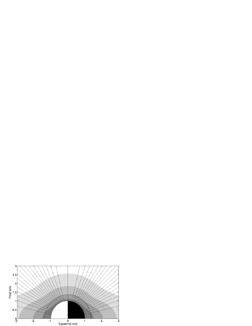
Figure 1: Poloidal fieldlines and density contours of the solution of Table 2 for model B. Distances are given in solar radii. The solid circle line indicates the Alfvén singularity and the fast magnetosonic separatrix which are almost coincident.

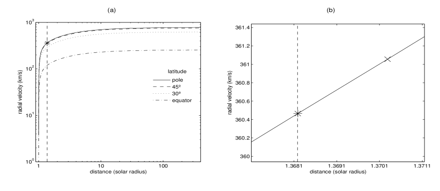
Figure 2: Panel (a) polar radial velocity as a function of distance. Panel (b) a zoom view of the singularities: the Alfvén and the fast critical points, represented by $\ast$ and $\ \times$ respectively.

Our procedure for finding a critical solution, using model B, that fulfills all criteria is thus:

• By fitting Ulysses data at 1 AU obtain the anisotropy parameters, $\epsilon$, $\delta$ and $\mu$, and the values $B_{1\rm{AU}}$, $B_{T,1\rm{AU}}$, $\rho_{1\rm{AU}}$ and $V_{1\rm{AU}}$;

• calculate $R_{\odot}$, $\lambda$ and $\nu$ with $f_{1\rm{AU}}=1$ and using Eqs. (18) to (20);

• with an initial guess of $\eta$, determine the values of $V_{*}$ and $B_{*}$ from Eqs. (15) and (16);

• at this stage it is possible to build a critical solution using the criteria of acceleration continuity at the critical points;

• this solution will give new values for the solar surface radius and for the different physical quantities at 1 AU;

• iterate until the computed values of the solar surface radius and velocity at 1 AU are close to the fitted ones.

Two convergence criteria are inherent to this procedure, the distance of the Alfvén surface above the Sun (or, equivalently, the value of the magnetic field strength at 1 AU – see Eq. 18) and the velocity at 1 AU. Satisfying all the criteria only by changing $\eta$ is not possible. Therefore, this can only be achieved by changing, in addition, at least one of the parameters, thus releasing one of the constraints. Considering that there are five constraints given from the data fit, exploring all the parameter space is a formidable task. The set of parameters concerning the best possible solution is presented in Table 2. This will be discussed in the following section.

3.2 Results

As can be seen in Table 2 we have constructed a solution where the convergence criteria are quite well fulfilled with input/output ratios very close to unity for all physical quantities. In Fig. 1 we show the fieldlines and the density contours in the poloidal plane. In Fig. 2, where the vertical dashed line represents the Alfvén radius, the acceleration at the critical points is clearly continuous. Note the presence of two different critical points, very close to one another in Fig. 2 (b). However, searching for a converged solution led us to this single set of parameters by using a value of the radial magnetic field, $B_{1\rm{AU}}$, of the order of one tenth of the value measured by Ulysses. A similar discrepancy was also found in SLIT05 using the STT99 model instead of LPT01 model. Moreover, the parameter that evaluates the anisotropy of the radial magnetic field, $\mu$, has also suffered a shift in its value (compare Table 1 to Table 2). As mentioned above we have tried to change the other input parameters and calculate their influence on the solution. The best option was to change those two parameters. Although these trials have been nearly exhaustive, degenerated sets of the input parameters for the same critical solution may be possible. In Fig. 3 we show the temperature profiles at various latitudes. The higher effective temperature along the polar axis corresponds to the fast solar wind. At lower latitudes the lower temperature is related to a mixing between the fast and slow wind, which also corresponds to the lower velocities seen in Fig. 2 (a). The temperature distribution is similar to the one presented in SLIT05 although its maximum value is slightly better, around $10\times 10^{6}$.

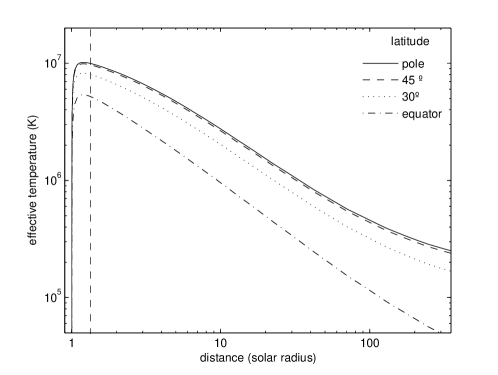
Figure 3: Effective temperature as a function of distance for different values of latitude for the model B solution. The vertical dashed line represents the Alfvén radius.

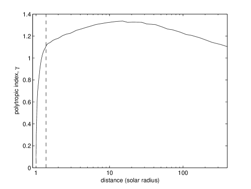
Figure 4: Polar polytropic index as a function of distance for the model B solution. The vertical dashed line represents the Alfvén radius.

We have also calculated the effective polytropic index of this solution. After the temperature peak, it is almost constant, between $1.1$ and $1.3$ (see Fig. 4). This value is quite close to the value inferred by Kopp and Holzer (1976) in their early polytropic model. Despite the difference between model A and B in their geometry, neither can reproduce from the observations the high value of the magnetic field inferred at 1 AU. The calculations were made such that we keep the temperature as low as possible and a reasonable value of the magnetic dipolar field at the base of the corona. We reproduce successfully the temperature and the velocity profile at 1 AU. It seems that the geometry does not control the decrease of the magnetic field but rather the temperature profile. It is even more surprising that in this LPT01 solution the density at 1 AU remains at a reasonable level, thus both the velocity and the mass flux at 1 AU correspond to the observed values. It is thus more consistent to build an hybrid solution combining both models A and B.

4 Hybrid solutions

4.1 Method for a solution

For the construction of the hybrid model we consider two different domains, one from the solar surface to the Alfvén radius, and the other from the Alfvén radius towards infinity. In the first domain we use model A, since the 3D structure is more able to describe the wind structure near the solar surface. Although the latitudinal functions of model A are not very versatile it does provide a full 3D description of the flaring. In the domain further out, where the fieldlines are almost radial in the poloidal plane, we can use model B and take advantage of its flexibility in fitting very steep variations of the physical quantities with latitude. The border between these two different domains was arbitrarily set at the Alfvén surface.

The major drawback of this construction is that we cannot guarantee continuity of all physical quantities everywhere except along the polar axis. Generating the critical solution with model A means that it must cross both slow magnetosonic separatrix critical point and Alfvénic singular point. In addition, the critical solution with model B has to cross the Alfvén point and a fast separatrix critical point. Thus, a new feature of this hybrid model compared to our previous solutions (SLIT05 and Sect. 3) is the crossing of the three usual MHD critical points. Such a situation was present only in the over-pressured solutions presented in STT04. Since for the solar wind the fast point is close to the Alfvén one, this was one more argument to construct the hybrid solution starting precisely at this Alfvénic transition. Moreover, in order to match the two solutions we must search for continuity of the physical quantities at the boundary as much as possible. This means that at the Alfvén surface we ask for continuity of the density, pressure, velocity and magnetic field plus continuity of the acceleration and fieldline geometry. Strictly speaking, this can only be done along the polar axis because the latitudinal dependences of the physical quantities are not identical in both models. Mathematically, we have

$${\rho^{modelA}_{*}}={\rho^{modelB}_{*}}$$ (21)

$$\Pi_{*}^{modelA}+C=\Pi_{0,*}^{modelB}$$ (22)

$${V^{modelA}_{*}}={V^{modelB}_{*}}$$ (23)

$${B^{modelA}_{*}}={B^{modelB}_{*}}$$ (24)

$${\frac{dY}{dR}^{modelA}_{\mid_{r_{*}}}}={\frac{dY}{dR}^{modelB}_{\mid_{r_{*}}}}$$ (25)

$${\frac{df}{dR}^{modelA}_{\mid_{r_{*}}}}={\frac{df}{dR}^{modelB}_{\mid_{r_{*}}}}=0$$ (26)

The technique used to obtain a full hybrid solution is as follows. First, the radial velocity at the Alfvén point, $V_{*}$, is determined by the same procedure as in the previous section. Then, the model A critical solution has to cross the slow separatrix critical point and the poloidal fieldlines have to be radial at the Alfvén point, Eq. (26). This yields the value of the velocity slope (i.e. the acceleration) at that transition point. Similarly, the value of the acceleration at the Alfvén point is determined by crossing the fast separatrix critical point for the critical solution of model B. In order for this slope of the velocity to be equal on both sides of the transition point, Eq. (25), the value of $\mu$ had to be changed from the one derived from Ulysses data. However this parameter is not very well determined and affects only model B. In model A its value is fixed to $-1$ by construction and cannot be fitted. For model A, knowing the slope of the velocity, Eq. (25), and the geometry, Eq. (26), at the Alfvén point, the value of $\Pi_{*}$ is fixed by crossing the Alfvén point. Simultaneously, the value of $\Pi_{0}$ is fixed by the condition that the pressure is zero at infinity. This determines the constant $C$ by Eq. (22). Finally, the Alfvén distance is fixed by the magnetic field strength at 1 AU for both models, Eq. (18). Thus, the value of $\kappa$ is determined such that the solution of model A matches the solar surface, $R_{\odot}$.

4.2 Results for a hybrid solution - hybrid 1

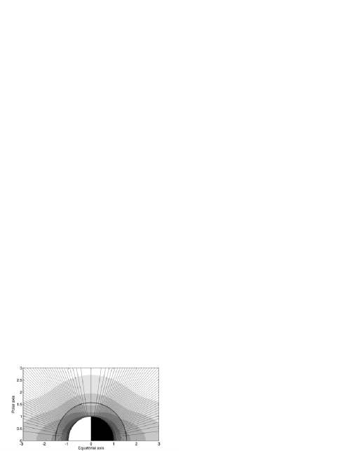
Figure 5: Plot of the fieldlines concerning the hybrid solution and density contours presented in Table 2, column 3, (hybrid 1). Distances are given in solar radii. The black circles corresponding to the slow magnetosonic critical separatrix, the Alfvén singularity and the fast magnetosonic critical separatrix, which almost coincide with each other.

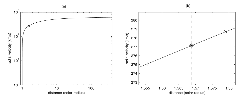
Figure 6: Panel (a) the polar radial velocity as a function of distance for solution hybrid 1. The vertical dashed line is at the transition point (Alfvén point). Panel (b), a zoom view of the three critical points is displayed. The slow magnetosonic, the Alfvén and the fast magnetosonic critical points are labelled with $+$, $\ast$ and $\times$, respectively.

Table 2 shows the input and output values for the most important physical quantities regarding the first hybrid solution obtained using the technique presented in the previous section. In this case convergence between the input and output parameters is less satisfying than in Sect. 3. This solution is hereafter referred to solution hybrid 1. Figure 5 shows the geometry of the fieldlines for this solution. It clearly shows that beyond the Alfvén point the fieldlines become radial in the poloidal plane and that the flaring zone near the base of the wind is well defined. Thus conversely to SLIT05 where the dead zone was too extended, we have a more realistic geometry. Figure 6 shows the polar radial velocity where the vertical dashed line represents the Alfvén radius, which corresponds to the border between application of models A and B.

The presence of three critical points characterizes a different topology for this kind of wind solution (similar cases were already discussed in STT04). Figure 7 shows the profile of the temperature for this solution. It is in reasonably good agreement with observations, namely at 1 AU. The polytropic index is shown in Fig. 8. It shows, as expected, that a value around 1.2 is very well adapted to the solar wind, except in the low corona. However, as we shall discuss in next section, this first hybrid solution suffers from the same drawbacks as the previous one, despite its more sophisticated structure. In addition, the density is too low by one order of magnitude. Thus, although the temperature profile is low enough to be in agreement with observations, the mass flux at 1 AU remains too low. The low effective temperature does not prevent us from obtaining large velocities but rather from obtaining large magnetic field at large distances. Thus we reconsidered the values of some of the parameters, in particular the value of the latitudinal dependence of the pressure which is not very well constrained from the observations, to construct another hybrid solution more fitted to the observed magnetic field.

Another way of analyzing the drawback of this solution is to examine the convergence of the value $r_{\odot}/r_{*}$. It represents by itself the convergence of the radial magnetic field intensity at 1 AU, Eq. (18).The convergence of the values of the Alfvén Mach number and density at this point, Eqs. (15) and (16), follows as a consequence. Ulysses data at 1 AU lead to a very high value of $R_{\odot}=r_{\odot}/r_{*}$ which, in turn, means that the acceleration of the wind up to the Alfvén speed should take place on a larger scale than the model predicts. Thus, a more satisfying solution should display a lower total acceleration from the surface up to the Alfvén point. The fully radial model used (see Sect. 3) is not able to produce that kind of behaviour. Some degree of flaring is needed in order to slow down its acceleration. Hence, the only way to deal with the problem is to decrease the acceleration zone by decreasing the value of $B_{r}$ at 1 AU, from Eq. (18). On the other hand, in model hybrid 1, the high density gradient near the equator (a consequence of the high values of $\epsilon$ and $\delta$) provides a poloidal pressure towards the pole, improving the polar collimation and subsequent acceleration of the wind. Therefore, the equatorial gradient of the radial magnetic field must increase ($|\mu|$ must increase), generating a higher magnetic pressure towards the equator which counterbalances the previous effect.

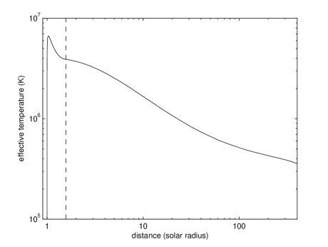
Figure 7: Effective temperature as a function of distance for the polar axis, for solution hybrid 1. The vertical dashed line represents the transition point between the use of model A and B.

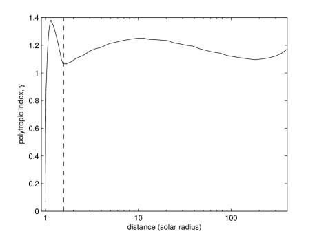
Figure 8: Radial profile of the polytropic index for solution hybrid 1. The vertical dashed line represents the transition point between the use of model A and B.

This wind solution needs a value for the magnetic field anisotropy parameter, $\mu$, very different from the one expected. It cannot easily describe the latitudinal profiles of the physical quantities from Ulysses data at 1 AU. Its main limitation (besides the temperature, to which we will refer later) is its discrepancy on the value of radial magnetic field. Both radial and hybrid solutions fail completely in reproducing the observed values of the the magnetic field but the hybrid solution also has a problem in reproducing the density at 1 AU. This lead us to construct the hybrid solution in a slightly different way.

4.3 Results for a fully converged hybrid solution - hybrid 2

In Table 2 we show the input and output values of the most important physical quantities, for a second hybrid solution - hereafter referred to solution hybrid 2. Although we had to release some of the initial values of the parameters as deduced from SLIT05, this new solution shows a much better agreement between the initial guesses and the computed values.

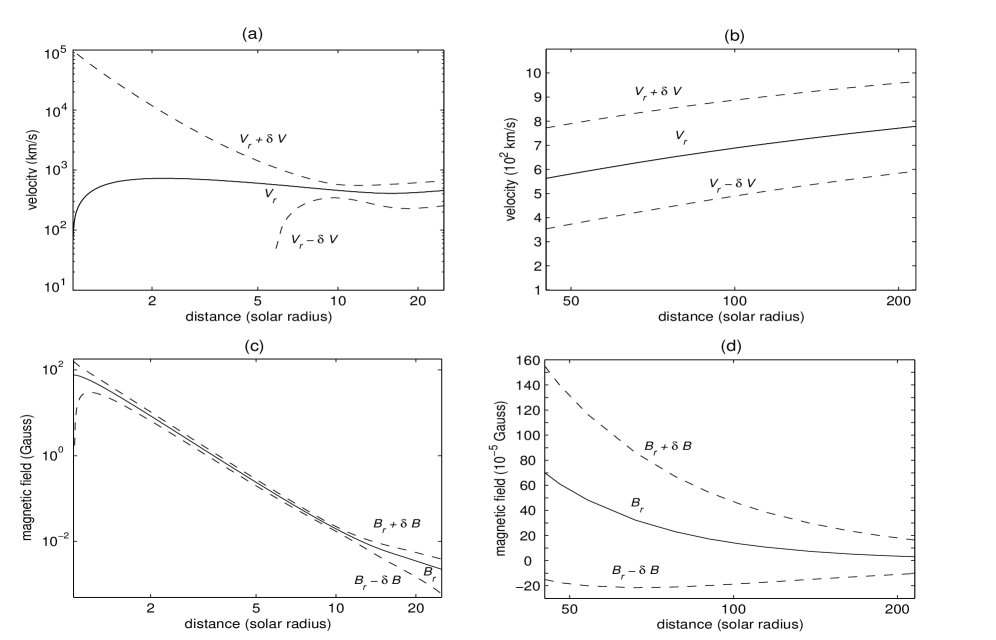
Figure 14: Assuming that turbulence and/or Alfvén waves can account for the effective temperature of the solutions, the corresponding bulk radial velocity plus and minus the velocity fluctuations. (a) near the solar surface and (b) close to 1 A.U. The magnetic field fluctuations, assuming Alfvén waves, in (c) near the solar surface and (d) close to 1 A.U.

For this solution, we had to change the value of $\kappa$ and of $\delta$, although in a less dramatic way. Changing the value of $\kappa$ in the sub-Alfvénic regime is not a serious problem. First because, in the super-Alfvénic region where the value of $\kappa$ is determined for the Ulysses data, we use model B in which we have no control over the latitudinal dependence of the pressure. Second, fitting the value of $\kappa$ in this domain is almost irrelevant as we do not really control the kinetic temperature (and pressure) which is the real temperature measured by the spacecraft. This discrepancy in the parameter can easily be evaluated by comparing input and output values of the same flow quantities. Figs. 9 and 10 show the geometry of the fieldlines and how it changes from model A to model B. A new feature of this solution can be seen in Fig. 11 (a) - a zone where the radial velocity attains a local minimum, close to the Alfvén point. Figure 12 displays the effective temperature profile along the polar axis. This plot clearly shows that the kinetic pressure alone cannot account for the effective temperature. Figure 13 shows the corresponding polytropic index. The excess between this temperature and the observed one can be accounted for, as in SLIT05, assuming extra pressure from Alfvén waves or turbulent or ram pressure (Fig. 14). We have calculated the amplitude of the ram velocity/magnetic field fluctuations, if the effective temperature we have calculated is assumed to be the result of turbulence/Alfvén waves. For ram pressure we assume:

$$P_{\rm{ram}}=\frac{1}{2}\rho\delta V^{2},$$ (27)

and for the Alfvén pressure we take

$$P_{\rm{Alfven}}=\frac{\delta B^{2}}{8\pi},$$ (28)

These calculations are arbitrary and a mixing of various processes is probably the source of the extra pressure that accelerate the fast wind. However it gives an order of magnitude of the fluctuations needed. Comparing the various plots a), b), c) and d) in Fig. 14, we conclude that Alfvén waves are more appropriate to explain the acceleration in the sub-Alfvénic part where the magnetic field is dominant. Conversely, turbulence and fluctuations of the velocity may account for the acceleration in the super-Alfvénic region. We arrive at this conclusion only because the calculated fluctuations of the magnetic field in the sub-Alfvénic region are smaller than the calculated turbulent velocity field and the reverse holds in the super-Alfvénic part. This is the best way to minimize the amplitude of the fluctuations in both regions. A mixture of the two components is probably more realistic but this needs a more detailed model to interpret the role of turbulence in heating the flow.

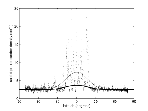
Figure 15: Scaled proton density with latitude. The points represent hourly averaged data from the Ulysses Swoops Ions experiment. The solid curve corresponds to the fit using model B and the bold solid curve to the solution generated by solution hybrid 2.

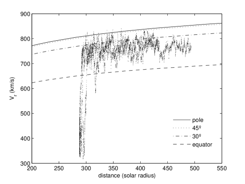
Figure 16: Radial velocity with distance to the Sun. The points represent hourly averaged data from the Ulysses Swoops Ions experiment. The curves correspond to the radial velocity at different latitudes of the solution generated by solution hybrid 2.

This new hybrid solution generates a field geometry that is continuous at the transition point (it is still not differentiable and kinks in the field are unavoidable) and shows features expected for the solar wind (Figs. 5 and 9). It is also capable of reproducing almost all Ulysses data at 1 AU. Despite the slight difference between the values of the anisotropy parameters when calculated by fitting the data (Table 1) and the one from the critical solution itself (Table 2), most of the limitations of the previous solutions have been solved. Such a discrepancy should not be very important since the new values can easily be fitted (with some degree of accordance) to the observed data (see for instance the fit of the density in Fig. 15 and of the radial velocity in Fig. 16). The ratio between the input and the output values for the most important physical quantities is very close to unity and all the continuity criteria are satisfied. Nevertheless, $\kappa$, $\delta$ and $\mu$ have values departing from the expected ones. The value of $\mu$ is the result of the transition conditions stated in Eqs. (21) to (26) and has been calculated accordingly.

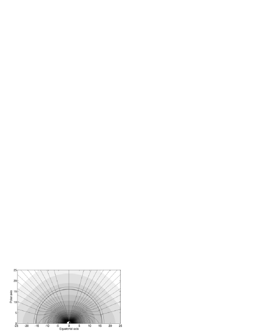
Figure 9: Fieldlines and density contours concerning the hybrid solution presented in Table 2 (hybrid 2). Distances are given in solar radii. The three black circles represent the three surfaces: the slow magnetosonic separatrix and Alfvén singularity, which are almost coincident, and a fast magnetosonic separatrix.

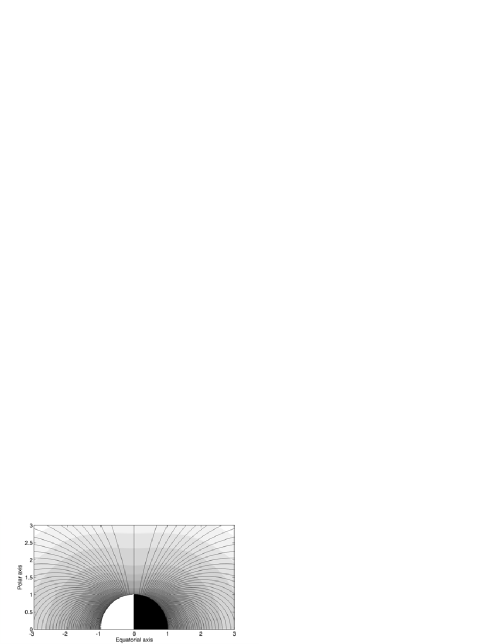
Figure 10: Fieldlines and density contours for solution hybrid 2, close to the solar surface. Distances are given in solar radii.

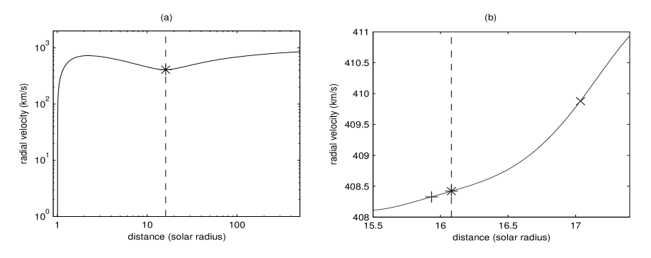
Figure 11: Panel (a) the polar radial velocity as a function of distance for solution hybrid 2. The vertical dashed line is at the transition point (Alfvén point). Panel (b), a zoom view of the three critical points: the slow magnetosonic, the Alfvén and the fast magnetosonic critical points, labelled with $+$, $\ast$ and $\times$, respectively.

The values of the magnetic field intensity at 1 AU constrain the value of $R_{\odot}$, and therefore the length of the wind acceleration zone (or the dead zone). Consequently, the physics controlling the hybrid model forced us to adapt it in order to obtain the required feature. Reminding that $\kappa$ and $\delta$ characterize the anisotropy of the pressure and density, decreasing both parameters will lead to a decrease of the pressure gradient towards the pole, which enables the wind to accelerate more slowly (from the solar surface to the Alfvén point). As a consequence of acceleration continuity at the transition point, $|\mu|$ also diminishes which means that the magnetic pressure gradient towards the equator, outside the Alfvén sphere (in the fully radial zone of the model), also decreases. For the dynamics of the radial part of the hybrid model, the wind velocity is expected to be higher in order to satisfy the values at 1 AU and so it needs to accelerate the wind. This leads to a decrease in the magnetic pressure towards the equator and thus a decrease of $\mu$.

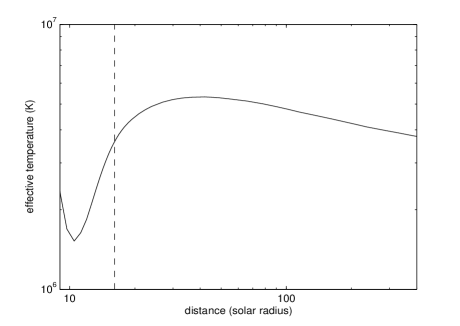
Figure 12: Effective temperature as a function of distance for the polar axis, for solution hybrid 2. The vertical dashed line represents the transition point between the use of model A and B.

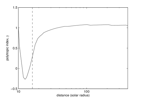
Figure 13: Radial profile of the polytropic index for solution hybrid 2. The vertical dashed line represents the transition point between the use of model A and B.

Of course, there is a price to pay to fit all data at 1 AU. Thus, this hybrid model has two major drawbacks. The physical quantities are discontinuous at the transition radius except for the polar ones. This is a natural consequence of the analytical expressions that describe the flow, Eqs. (1) to (14) and the temperature behaviour. The first one is solved only for values of $\epsilon=1$. The second and more serious drawback is the very high effective temperature. This can be explained only if we calculate the heat flux using a reasonable kinetic theory (Zouganelis et al., 2005) together with solving a full energy equation. This amounts to invoking a non thermal heating term, a difficult task that we postpone for future work. In Fig. 12, we see how the energy equation can be essential. The absence of the an abrupt increase of the temperature very close to the surface in other models, such as the one presented in SLIT05 and the one presented in Sect. 3 of the present work might be explained by solar surface being much closer to the Alfvén radius and therefore the problems had not emerged yet. Nevertheless, high temperatures are reached (for an overall behaviour of the wind solution) as a consequence of high values of the magnetic field at 1 AU and not necessarily high values of velocity as one may expect intuitively.

5 Conclusions

From the constrained parameters obtained after fitting Ulysses data (SLIT05) we were able to build different critical solutions for the solar wind. The first was obtained using a purely radial field (model B). The remaining two solutions where constructed as hybrid ones incorporating an inner region where model A (with flaring streamlines) was used and an outer one with model B. Thus, we combine the advantages of model B of reproducing highly adaptable functions of latitude and the advantages of model A of ensuring adequate flaring of the fieldlines to get a more realistic geometry of the overall solar wind. These two distinct models were coupled using well defined domains for each one and a suitable transition zone, the Alfvén radius. Both model B (used by itself) and the hybrid model (A and B coupled) were used to generate a critical wind solution that could replicate the measured values of some important physical quantities, such as the radial velocity, the radial and toroidal magnetic fields and the density, at 1 AU measured by Ulysses at solar minimum.

In the hybrid model, we could not avoid some discontinuity out of the polar axis. This may be solved in the future by using the present solutions to start more realistic MHD simulations. For the first model with helicoidal streamlines, the computed velocity and density values at 1 AU are in good agreement with Ulysses data. However, we were clearly not able to reproduce the values of the radial magnetic field. This is also true for the first hybrid model we presented (hybrid 1), which in addition failed to reproduce the density at 1 AU by one order of magnitude. This can be understood because we tried to minimize the temperature along the flow. The second hybrid model is able to reproduce the values of all physical quantities at 1 AU except for the temperature. This is too high even though we can invoke non thermal processes to explain the excess of effective pressure. It also provided a solution with a smooth geometry where the fieldlines became purely radial after the Alfvén radius. Some concessions were made in the values of the parameters that rule the dynamics of both models. They are slightly different from the ones calculated in the method presented in SLIT05. Such differences can be explained by the physics that describes the dynamics of the flow. Even though the high values of the temperature at 1 AU can be explained (SLIT05), its behaviour close to the solar surface suggests the implementation of an energy equation. Since this is a formidable task, we postpone it for future work. However, we face the same difficulties as any MHD simulation. The main advantage of the present solutions is its simplicity. Moreover, they are exact solutions of the ideal MHD equations.

References

- Acuna et al. (1995) Acuna M.H., Ogilvie K.W., Baker D.N., et al.: 1995, Space Science Reviews 71, 5
- Cuperman et al. (1990) Cuperman S., Ofman L., Dryer M.: 1990, ApJ 350, 846
- Gallagher et al. (1999) Gallagher P.T., Mathioudakis M., Keenan F.P., Phillips K.J.H., Tsinganos K.: 1999, ApJ 524, L133
- Grappin et al. (2002) Grappin R., Léorat J., Habbal S.R.: 2002, Journal of Geophysical Research (Space Physics) 107, 16
- Groth et al. (1999) Groth C.P.T., de Zeeuw D.L., Gombosi T.I., Powell K.G.: 1999, Space Science Reviews 87, 193
- Hayashi (2005) Hayashi K.: 2005, ApJS 161, 480
- Keppens & Goedbloed (2000) Keppens R., Goedbloed J.P.: 2000, ApJ 530, 1036
- Kopp & Holzer (1976) Kopp R.A., Holzer T.E.: 1976, ^ 49, 43
- Landi & Pantellini (2003) Landi S., Pantellini F.: 2003, A&A 400, 769
- Lewis & Simnett (2002) Lewis D.J., Simnett G.M.: 2002, MNRAS 333, 969
- Lima et al. (2001) Lima J.J.G., Priest E.R., Tsinganos K.: 2001, A&A 371, 240
- McComas et al. (2000) McComas D.J., Gosling J.T., Skoug R.M.: 2000, Geochim. Res. Lett. 27, 2437
- Nerney & Suess (2005) Nerney S., Suess S.T.: 2005, ApJ 624, 378
- Ofman (2000) Ofman L.: 2000, In: AIP Conf. Proc. 537: Waves in Dusty, Solar, and Space Plasmas, p. 119
- Parker (1958) Parker E.N.: 1958, ApJ 128, 664
- Pneuman & Kopp (1971) Pneuman G.W., Kopp R.A.: 1971, Sol. Phys. 18, 258
- Sauty et al. (2005) Sauty C., Lima J.J.G., Iro N., Tsinganos K.: 2005, A&A 432, 687
- Sauty et al. (2002) Sauty C., Trussoni E., Tsinganos K.: 2002, A&A 389, 1068
- Sauty et al. (2004) Sauty C., Trussoni E., Tsinganos K.: 2004, A&A 421, 797
- Sauty et al. (1999) Sauty C., Tsinganos K., Trussoni E.: 1999, A&A 348, 327
- Sittler & Guhathakurta (1999) Sittler E.C., Guhathakurta M.: 1999, ApJ 523, 812
- Steinolfson et al. (1982) Steinolfson R.S., Wu S.T., Suess S.T.: 1982, ApJ 255, 730
- Stone et al. (1998) Stone E.C., Cohen C.M.S., Cook W.R., et al.: 1998, Space Science Reviews 86, 357
- Tsinganos & Sauty (1992) Tsinganos K., Sauty C.: 1992, A&A 255, 405
- Tsinganos et al. (1996) Tsinganos K., Sauty C., Surlantzis G., Trussoni E., Contopoulos J.: 1996, MNRAS 283, 811
- Usmanov & Goldstein (2003) Usmanov A.V., Goldstein M.L.: 2003, Journal of Geophysical Research (Space Physics) 108, 1
- Vlahakis et al. (2000) Vlahakis N., Tsinganos K., Sauty C., Trussoni E.: 2000, MNRAS 318, 417
- Wang & Sheeley (2003) Wang Y.M., Sheeley N.R.: 2003, ApJ 599, 1404
- Woo & Gazis (1994) Woo R., Gazis P.R.: 1994, Geochim. Res. Lett. 21, 1101
- Woo & Habbal (2005) Woo R., Habbal S.R.: 2005, ApJ 629, L129
- Zouganelis et al. (2004) Zouganelis I., Maksimovic M., Meyer-Vernet N., Lamy H., Issautier K.: 2004, ApJ 606, 542
- Zouganelis et al. (2005) Zouganelis I., Meyer-Vernet N., Landi S., Maksimovic M., Pantellini F.: 2005, ApJ 626, L117