Abstract

The shifting of spectral lines due to induced correlation effect, discovered first by Wolf for the single scattering case which mimics the Doppler mechanism has been extended and developed further by the present authors to study the behavior of spectral lines in the case of multiple scattering and observed shifting, as well as broadening of the spectrum. We have explored Dynamic Multiple Scattering(DMS) theory for explaining anomalous redshifts in quasars. Our recent work, based on the statistical analysis of the Véron-Cetty data(2003) supports that quasar redshifts fit the overall Hubble expansion law, as in the case of galaxies, for $z\leq 0.295$ but not for higher redshifts, indicating clearly the inadequacy of the Doppler effect as the sole mechanism in explaining the redshifts for high redshift quasars($z\geq 0.295$). We found that the redshift posseses an additive,“discordant” component due to frequency shifting from the correlation induced mechanism which increases gradually for $\sim 0.295\leq z\leq 3.0$, however, appearing to follow the evolutionary picture of the universe with absolute dependence on the physical characteristics i.e., environmental aspects of the relevant sources through which the light rays pass, after being multiply scattered. According our framework, as the environment around sources is diverse, subject to the age of the universe, it determines the amount of multiple scattering effect, probably, without additional additive effects for higher values i.e., for redshifts  $3.00\leq z$. The recent observational data on redshift $z$ versus apparent magnitude($m$) (Hubble like relation) are found to be in good agreement, considering suitable values of the induced correlation parameters. This resolution of the paradox of quasar redshifts is much more appealing and in a sense, more mainstream physics than either assigning redshift entirely to the Doppler effect or inventing a new, often unknown, physical mechanism. Our analysis indicates the importance of local environmental aspects of relevance (recent observations of molecular gases, the plasma like environment, evolution of the hydrogen content with epoch etc.) around quasars, especially for the higher redshift limits. Our work opens possible new vistas in quasar astronomy as well as for cosmological models of the universe.

Dynamic Multiple Scattering, Frequency Shift and

Possible Effects on Quasars Astronomy

Sisir Roy^1,2, Malabika Roy¹, Joydip Ghosh¹ & Menas Kafatos¹

¹Center for Earth Observing and Space Research, School of Computational Sciences,

George Mason University, Fairfax, VA 22030 USA

²Physics and Applied Mathematics Unit, Indian statistical Institute, Kolkata, INDIA

e.mail: ¹ mkafatos@crete.gmu.edu
e.mail: ¹ sroy@scs.gmu.edu

keywords Dynamic Multiple Scattering, Doppler shift, Quasars, Hubble law [Running Title: Dynamic Multiple scattering]

1 Introduction

The frequency shift of spectral lines is most often attributed to the Doppler effect, and the Doppler broadening of a particular line depends on the temperature, pressure or the different line of sight velocities. In the last few years, a dynamic multiple scattering theory^1,2 has been developed to account for the shift as well as the broadening of spectral lines, even in the absence of any relative motion between the source and the observer. This development followed the theoretical prediction made by Wolf^3,4 who discovered that under appropriate circumstances, it is possible to have frequency shifts of spectral lines which typically mimic all the characteristics of the frequency shifts obtained by the Doppler mechanism. Since then, it has been verified by experiments^5,6 that, contrary to a commonly held belief, the spectrum of light is, in general, not invariant on propagation through a medium, especially, for anisotropic (i.e., inhomogeneous) medium with fluctuations of the dielectric susceptibility, both temporal and spatial. For example, if radiation is scattered by some scatterer, the spectrum may change; its maximum may shift either to the red or to blue part of the spectrum, depending upon the physical parameters involved in the process. It is well known fact that at higher temperatures, more energy is concentrated in the high-frequency part of the spectrum(Planck distribution). According to Wolf^3,4,7, this distribution is not universal:  the spectrum can change if the source is partially coherent with respect to the spatial and temporal coordinates. Wolf^3,4, and subsequently others examined about the possible implications^1,2,8-15. These conditions are generally found in the case of light passing through an anisotropic, weakly turbulent(tenuous) i.e., some kind of inhomogeneous medium. In such case, the shift as well as the broadening of the spectral lines can be caused by the induced correlation mechanism within the medium¹⁶. An intuitive understandings of this effect has been elaborated further by Tatarskii¹⁷. Following this framework, sufficient conditions for redshift (i.e., when the shifting is larger than broadening), also known as no-blue shift condition¹⁸, have been derived by Datta et al.^1,2. They also calculated the critical condition for the source frequency¹⁹ under which the spectrum will be analyzable without blurring. Recently, it has been pointed out by several authors^11-13,19-21 that this mechanism may explain the anomalies in observed redshift measurements especially in the case of quasar astronomy. It is generally believed that the medium around a quasar is a highly anisotropic and plasma like (i.e., can be considered as underdense). The paper is organized as follows : before entering into the details of the problem, we describe, as a background, the correlation induced mechanism and dynamic multiple scattering in section II and III, respectively. Section IV deals with the impact of the environment on the incident radiation, emerging from of a source, on the spectral line width of the spectrum traversing the medium and consequently on redshift observations. The width of the spectral line is calculated after multiple scatterings and the contribution of this mechanism on the variation of the width with redshift ${z}$ is studied in quasar astronomy, especially, in the case of quasars where the nature of observed variation is difficult to explain. Using the relation of width and ${z}$,  Roy et al.⁽⁸⁾ has already established a generalized relation for distance modulus which can be reduced to a Tully-Fisher type relation, as the contribution due to Wolf effect becomes almost negligible for low redshifts. Ultimately, this points to the possible impacts on the Hubble diagram itself, especially, when we approach higher redshifts ($z\geq 0.3$). The Hubble flow for the standard cosmological models is considered and a comparison is made with the Hubble Law, following our framework and also the statistical fitting based on the nonparametric statistical analysis and regression. The clear deviation of the linear Hubble law for high redshift ($z$) quasars is explained in our framework for a certain range of medium parameters i.e., $\alpha,\alpha^{\prime}$ and $\beta$. However, this kind of deviation (or the existence of a bulge) has already been mentioned by several authors in connection with the Hubble diagram for high redshift Supernovae^(22),(23). Our analysis clearly indicates that, in addition to observed redshifts, caused by the Doppler and/or gravitational effects, some quasars may contain contributions due to presence of the induced correlation properties inside the fluctuating medium, arising from intrinsic properties of the medium surrounding the radiating sources. Finally, in section V and VI, we discuss possible implications and conclusions regarding the application of the presently discussed mechanism to quasar astronomy and cosmology in general.

2 Correlation Induced Mechanism : Nature of the Source and the Medium

2.1 Dielectric Response in a Random Medium with spatial and Temporal Fluctuation

The scattering of electromagnetic waves by a random medium involves the solution of Maxwell’s equations and an ensemble average over random fluctuations. Such calculations can be carried out for the first order Born approximation. Recently a Japanese group^14,15 showed that the higher order Born approximations contribute of negligible amount in case of multiple scattering in a random, tenuous medium. In this case, i.e., in the first order Born approximation, the medium is treated as tenuous which means the filling factor, i.e., the ratio of the volume occupied by particles to the total volume of the medium, is considerably smaller than $0.1\%$. When it becomes much greater than $1\%$, the problem is to be treated as diffusion, but in the neighborhood of $1\%$ neither of the two treatments is valid and it requires a solution considering the complete equation of transfer. Thus the present case is for a medium in which the dielectric constant, permeability and the conductivity are all random functions of position and time. Strict homogeneity requires, of course, that the medium occupies all space. However, in the present case, we assume that the linear dimensions of the domain are very large compared to the distances over which the correlations of the fluctuations in the macroscopic physical properties of the medium are non-negligible. Also, we consider the dielectric response in a very weakly fluctuating random medium. Let us begin by recalling some standard relations between the electric field and the induced polarization in a linear inhomogeneous, isotropic and nonmagnetic medium. At the end, we will deal with the associated magnetic field too. The Fourier transforms are given by

$$\tilde{\bf E}({\bf r}\omega)=\frac{1}{2\pi}\int^{\infty}_{\infty}{\bf E}({\bf r},t)e^{(i\omega t)}dt$$

$$\tilde{\bf P}({\bf r},\omega)=\frac{1}{2\pi}\int^{\infty}_{\infty}{\bf P}({\bf r},t)e^{(i\omega t)}dt$$

of the real electric field ${\bf E}({\bf r},t)$ and the induced polarization ${\bf P}({\bf r},t)$ respectively²⁴. Here, ${\bf r}$ denotes the position vector and $t$ the time. ${\bf E}({\bf r},t)$ and ${\bf P}({\bf r},t)$ are related by a constitutive relation

$$\tilde{\bf P}({\bf r},\omega)=\tilde{\eta}({\bf r},\omega)\tilde{\bf E}({\bf r}\omega)$$ (1)

where $\tilde{\eta}({\bf r}$ denotes as the dielectric susceptibility, describing the response of the medium at the frequency $\omega$ of the incident wave. According to microscopic theory, $\tilde{\eta}({\bf r},\omega)$ can be expressed in terms of the average number ${\cal N}({\bf r})$ of molecules per unit volume present in the medium and the mean polarizability $\alpha(\omega)$ of each molecule by the Lorentz-Lorenz relation,

$$\tilde{\eta}({\bf r},\omega)={\bf{\cal N}}({\bf r})\alpha(\omega)[1-(\frac{4\pi}{3}){\bf{\cal N}}({\bf r})\alpha(\omega)]^{-1}$$ (2)

Let the dielectric constant $\epsilon_{r}$ be described by a random function of position and time

$$\epsilon_{r}=\epsilon({\bf r},t)=n^{2}({\bf r},t)$$ (3)

which in turn, is related with the dielectric susceptibility $\tilde{\eta}({\bf r}$ as

$$n^{2}(\omega)=1+4\pi\tilde{\eta}(\omega)$$ (4)

implying

$$\frac{4\pi}{3}{\cal N}\alpha(\omega)=\frac{n^{2}(\omega-1)}{n^{2}(\omega+2)}$$ (5)

The polarizability  $\alpha(\omega)$  is a causal, complex function of frequency and, consequently, its real and imaginary parts are coupled by dispersion relations²⁵. It contains the frequency dependence and plays a crucial role, especially, when dealing with the scattering of light waves in a plasma medium alone. In the present case, ${\cal N({\bf r}},t)$ is assumed to be real, stationary, homogeneous random function of position and time, of zero mean value. For dilute gas, ${\cal N({\bf r}},t)$  represents the density of molecules at the point ${\bf r}$  and time $t$, while $\alpha(\omega)$  represents the response of the individual molecules to the applied field oscillating with frequency $\omega$. The scattering from the plasma medium has been extensively studied by various groups using the first Born approximations. Watson^26,27, studied the multiple scattering of electromagnetic waves both in dense and tenuous plasmas. However, it is not trivial to relate the dielectric constant to the plasma properties. In the case of plasma, coherently interfering wavelets propagating in a medium with a refractive index $n$, can be expressed in terms of plasma correlation functions and density. On the other hand, the coherent scattering is usually described by ”classical like” transport equations^28,29. For the present case, we are dealing with the physical characteristics, as described here, without going into the full details of the plasma case. It is to be noted here that as there is substantial velocity of gas molecules or other particles present in the medium, and the velocity is a vector field , we need to construct a general structure function between different components. Also, we need to consider the effects of pressure, partial pressure, temperature etc. of a particular component like hydrogen. However, we take the Fourier transform of Eq.(1) and make use of the fact that the response of the medium is necessarily causal. Then, we can write the following constitutive relation :

$${\bf P}(t)=\frac{1}{2\pi}\int^{t}_{-\infty}\eta(t-t^{\prime}){\bf E}(t^{\prime})dt^{\prime}$$ (6)

or, equivalently

$${\bf P}(t)=\frac{1}{2\pi}\int^{\infty}_{0}\eta(t^{\prime}){\bf E}(t-t^{\prime})dt^{\prime}$$ (7)

where,

$$\eta(\tau)=\int^{\infty}_{-\infty}\tilde{\eta}(\omega)e^{-i\omega\tau}d\omega$$ (8)

In our case, we consider a medium where,  $\eta$  depends on time through  ($t-t^{\prime}$) instead of $t$ or $t^{\prime}$ and also $\eta(\tau)=0$ for $\tau<0$ because of the assumption of causality.
If the response of the medium is time dependent, the number density of the medium also changes with time and consequently, if temporal variation are not too strong , we have

$$\hat{\eta}({\bf r},t;\omega)=\frac{{\cal N}({\bf r},t)\alpha(\omega^{\prime})}{1-\frac{4\pi}{3}{\cal N}({\bf r},t)\alpha(\omega^{\prime})}$$ (9)

Though the precise range of validity of the above relation is heavily dependent on the microscopic considerations, it clearly points to the physical origin of the generalized dielectric susceptibility which depends on two rather than one temporal arguments, i.e., $\eta({\bf r},t;\omega)$  is a random function with respect to its first time argument and deterministic function with respect to its second time argument. For practical purposes, when the effective frequencies(say $\omega_{0}$)  of the electric field are not too close to any of the resonance frequencies of the medium, the random fluctuations of the scattering medium are taken to be stationary, at least in the wide sense³⁰ and the medium is also homogeneous so that we can arrive at an approximated formula as follows³¹:

$${\bf P}({\bf r},t)=\hat{\eta}({\bf r},t;\omega_{0}){\bf E}({\bf r},t)$$ (10)

It is this approximate nature of time dependent response function $\hat{\eta}(\bf r,t)$ which is responsible for determining its validity in the field which contains frequencies, near or far away from resonances. So, in this correlation induced mechanism, we have considered the random susceptibility $\eta$ as a function of $\omega,{\bf r},t$, and under these conditions, $\eta$  is of the approximate form

$$\eta(\omega,{\bf r},t)=\eta_{1}(\omega)\eta_{2}({\bf r},t)$$ (11)

Under suitable circumstances, one can be consider  $\eta(\omega)={\rm constant}$,  as effectively independent of $\omega$. This is analogous to the dynamic structure factor for particle density fluctuations²⁸.

2.2 Condition for the Change of initially incoherent radiation to a coherent spectrum after scattering

In discussing the propagation and scattering of an initially incoherent radiation, let us first try to understand what circumstances may change the initial spectrum. Let us consider, at first, that an initial spectrum is from an incoherent source. Now, some scatterer may be present having its size small compared to that of the source, at an arbitrarily large distance. Consequently, the scatterers can be considered as illuminated practically by a spatially coherent radiation. Electromagnetically, it can be described as a scattering phenomenon where radiation from the secondary dipoles fall on the scatterer under the influence of the incident wave. As the coherent source may distribute its energy in different directions, differently at different frequencies, then, in some directions, the scattered radiation may have a quite different (from the initial) distribution of the energy in frequency space, i.e., the Wolf shift may appear, as has also been concluded by Tatarsky¹⁷. Then, if for some reason, we do not observe the direct radiation(say, the angular distance between the primary source and scatterer is very large), but only a scattered one, we may conclude that the spectrum corresponds either to a red shift or a blue shift. In other words, an initially, spatially incoherent field becomes partially coherent at some distance, and the coherence radius increases with distance. This phenomenon is closely related to the theorem of Van Cittert³² and Zernicke³³. Also, in all wave fluctuation phenomena, irrespective of the form or nature of correlation function, if the correlation distance is much smaller than the Fresnel zone size $\sqrt{\lambda L}$, where $\lambda={\rm wavelength}$  and  $L$ is distance of the far zone of scattering, then in general, the amplitude and phase variances are equal and proportional to the square of frequency and to the distance $L$. But, if the correlation distance is much larger than the Fresnel zone, then the cross section becomes independent of frequency and proportional to $L^{3}$. Physically it means that for a short distance, the amplitude does not vary much but the phase does with the distance of wave propagation. But as the distance increases, the amplitude fluctuation also increases and practically there does not remain any difference between amplitude and phase fluctuations.

2.3 Effects of Fluctuation on the Behavior of the Field in the Medium

Many physical characteristics of the medium determine the behavior of the incoming or interacting field. One among them is the optical distance  $\gamma=\rho\ \sigma_{t}\ x$,  where,  $\rho$  is the density of particles,  $\sigma_{t}$  denotes the total cross section and $x$ the semi-infinite region  $(x>0)$³⁴,  respectively. For $\gamma<<1$,  the field becomes predominantly coherent whereas, when $\gamma\simeq 1$,  the opposite behavior arises (incoherent or fluctuating field). This causes an amplitude fluctuation behavior. However, we consider a medium with weak fluctuation where the field is predominantly coherent i.e., the degree of coherency is much more than that of incoherency, which means  $\gamma>>1$.  Another case can also be encountered in practice when the angle of scattering is very small and the role of coherent field(average field) dominates even with optical distances comparable to unity. In such a situation, the field can be considered as weakly fluctuating as the fluctuation can be taken as a stationary process which means the mean period and correlation time to be much shorter than the averaging interval needed to make the observation. Now, when an electromagnetic wave is incident upon a turbulent medium, the amplitude as well as the phase of the incident wave experience fluctuations due to the relative dielectric constant $\epsilon_{r}$ or the index of refraction  $n$ which can vary both spatially and temporarily in the case of turbulent medium (through Eq.(3) and (7)). According to the present framework, the medium around the radiating source is generally characterized by the permittivity $\epsilon({\bf r},t)$, which is a random function not only of space and time but also of other characteristics like pressure, temperature density of particles, degree of ionization etc., through the relation with refractive index, as explained earlier. It is evident from Eq.(2,3 & 4 ) that in any linear medium, the dielectric susceptibility can also be related to the dielectric co-efficient. Now, in the case of a random but weakly fluctuating medium, we can write

$$\epsilon({\bf r},t)=<\epsilon({\bf r},t)>(1+\epsilon_{1}({\bf r},t))$$ (12)

where, $\epsilon_{1}({\bf r},t)$  is the fluctuating part of the permittivity with  $<\epsilon_{1}>=0$. Also, the refractive index $n({\bf r},t)$  being a random function of space and time can be written as

$$n({\bf r},t)=\sqrt{\frac{\epsilon({\bf r},t)}{\epsilon_{0}}}=<n({\bf r},t)>[1+n_{1}({\bf r},t)]$$ (13)

$\epsilon_{0}$  being the free space permittivity, assumed to be constant and $n_{1}$, the fluctuating part of the refractive index. For small fluctuations i.e., considering a weakly fluctuating medium, we obtain

$$\epsilon_{1}({\bf r},t)\simeq 2n_{1}({\bf r},t)$$ (14)

When considering an ionized plasma medium, such as the ionosphere, it can be assumed ³⁴

$$\epsilon_{1}\simeq g\frac{\delta\rho}{\rho}$$ (15)

where,

$$g=-\frac{\omega_{N_{\rm e}}^{2}}{\omega^{2}};\ \ \ \ \omega_{N_{\rm e}}^{2}=(\frac{1}{\epsilon_{0}})(\frac{N_{\rm e}e^{2}}{m_{e}})$$

$N_{\rm e}$ is the number density of free electrons in the medium and $m_{e}$  being the mass of the electron. $\epsilon_{1}$  is assumed to be due to the fluctuations in electron concentration, proportional to the density $\Delta\rho$ of the carrier medium. Villars and Weisskopf³⁴ studied the scattering of electromagnetic waves in the ionosphere, with such an $\epsilon_{1}$ and showed that the scattering is compatible with observations. Therefore, for the case of small fluctuations,

$$2n_{1}\simeq g\frac{\delta\rho}{\rho}$$ (16)

Taking the average,

$$<n_{1}^{2}>\simeq\frac{g^{2}}{4}<\frac{\delta\rho}{\rho}\frac{\delta\rho}{\rho}>=\phi(\omega).f({\bf r},t)$$ (17)

Here, the time-dependence in $\delta\rho$ is assumed to lie outside the domain of propagated frequencies $\omega$, considering  $\phi$  is a function of frequency $\omega$ and, taking $f$  as a function of space and time only. In this way, even if, one considers the scattering from ionized plasma but, far away from resonance region, the correlation induced mechanism can be applied^24,35. Likewise, we assume that the correlation of refractive indices at two points in the ionized plasma medium (tenuous and underdense) can also be decomposed into two functions , a function of frequency and a function of space and time. It is to be mentioned, for the real value of $n^{2}$, there will be a sharp cut-off at the resonance. Otherwise, they will be diffused. There also will be a cut-off when the phase velocity approaches infinity and correspondingly $n^{2}=0$  e.g., at low frequencies ,  $\omega=\omega_{re}$.  In case of resonance, the phase velocity will be zero and $n^{2}\rightarrow\infty$.  Normally the sharpness condition is applied to collisionless plasma, but collisions can also be taken into account under certain conditions³⁵. However, we also need to consider other factors, such as, the dependence on the distance between source and scattering medium, the spatio-temporal fluctuation of structure functions, together with other characteristics of the medium, like, densities of different particles present, magnetic field strength leading to the variation of degree of ionization, etc. Now, within certain distance limit, when the intensity of the turbulence is weaker than a certain level, some mathematical simplifications are possible and the case can be referred as ”weak fluctuation” approximation. In this way, many processes encountered in practice can be approximated reasonably well within the domain of stationary or homogeneous random functions, even if, the approximation is only valid within a limited time or spatial distance. Mathematically, this kind of physical processes when treated as random functions are referring to a random process with stationary increments of a function of time and locally homogeneous random function of position and the description is done in a convenient way by taking a two point correlation function analogous to the so called Van Hove time dependent two-point correlation function^28,30,31  in neutron scattering, the medium being treated statistically in the behavior and consequences of the wave scattering.

3 Dynamic Multiple Scattering

The scattering of light induced by the random susceptibility which can produce both a shift and a broadening of the spectral lines, other than Doppler mechanism, has been studied in statistical optics³⁵, where the existence of a random dielectric susceptibility fluctuation, both spatially and temporally, is assumed. This is the so called Wolf effect^3,4. Following the above formalism, during the last decade, some closely related processes have been developed that can generate frequency shifts of spectral lines^1,2,9-13,18. Such spectral effects were first investigated in ^3,4 for the case of a static scattering medium; the analysis for the case of time-dependent scatterers followed soon thereafter^14,15. To start with, we briefly present the main results of Wolf’s scattering mechanism.

3.1 Single Scattering by Wolf Mechanism : Wolf Effect

Let us consider the case when both the source and the medium through which scattering occurs, to be randomly fluctuating. Together with this, we assume a polychromatic electromagnetic field of light of central frequency $\omega_{0}$ and width $\delta_{0}$, incident on the scatterer. The general dielectric susceptibility $\eta$, considered here, characterizes the response of the space-time fluctuating medium, and is given as a function of three variables :  the position vector ${\bf R}$ and the time  $\tau$ resulting from, i.e., thermal fluctuations of the medium and the frequency  $\omega$  of the incident field. More specifically, the correlation function is taken as homogeneous and stationary, at least in a general sense and with a zero mean, a generalized analogue of the Van Hove two-particle correlation function²⁸, frequently encountered in neutron scattering. Let the incident spectrum be assumed to be of the form³⁶

$${S^{(i)}(\omega)=A_{0}e^{\left[-\frac{1}{2\delta_{0}^{2}}(\omega-\omega_{0})^{2}\right]}}$$ (18)

The spectrum of the scattered field is given by⁽¹²⁾

$${S^{(\infty)}r({\bf u^{\prime}},\omega^{\prime})=A\omega^{\prime 4}\int_{-\infty}^{\infty}{\cal K}(\omega,\omega^{\prime},{\bf u},{\bf u^{\prime}})S^{(i)}(\omega)d\omega}$$ (19)

which is valid within the first order Born approximation^36-38. $A$, the spectral amplitude after being scattered, can be determined in terms of $A_{0}$, by

$$A_{0}=\frac{(2\pi)^{3}V(\sin^{2}\psi)}{c^{4}r^{2}}$$

where, $V$  represents the volume of the scattering medium (whose linear dimension is assumed to be large compared with the correlation width of the medium)  and  $\psi$ denotes the angle between the direction of the electric vector of the incident wave and the direction of the scattering, $c$ is the speed of the light in vacuum. ${\bf u}$ and ${\bf u^{\prime}}$ are the unit vectors in the direction of incident and scattered fields respectively. Here, ${\cal K}(\omega^{\prime},\omega;\textbf{u}^{\prime},\textbf{u})$  is the so called scattering kernel and plays the most important role in this mechanism, given by

$${\cal K}(\omega^{\prime},\omega;{\bf{u}^{\prime}},{\bf{u})}\equiv\widetilde{G}\left(\frac{\omega^{\prime}}{c}{\bf u}^{\prime}-\frac{\bf{u}}{c}\bf{u},(\omega^{\prime}-\omega);\omega\right)$$ (20)

with

$$\widetilde{G}(\textbf{k},\Omega;\omega)=\frac{1}{(2\pi)^{4}}\int_{V}d^{3}R\int^{\infty}_{\infty}dTG(\textbf{R},T;\omega)\times exp[-i(\textbf{k}.\textbf{R}-\Omega T)]$$

As the dielectric susceptibility is considered in a statistically homogeneous and stationary medium, the angular brackets in the correlation function  $<\hat{\eta}^{*}({\bf r_{1}},t,\omega^{\prime})\hat{\eta}({\bf r_{2}},t^{\prime},\omega^{\prime})>$  denote the average over an ensemble of the random medium depending on ${\bf{r_{1}}}$, ${\bf{r_{2}}}$ and $t,\ \ t^{\prime}$ only through the difference ${\bf{(r_{1}-\bf r_{2})}}$, and $(t^{\prime}-t)$,  respectively. Also, the medium where the character of the fluctuations does not change with time, even though any realization of the ensemble  $x(t)$  changes continually in time, is said to be statistically stationary. It means that all the ensemble averages are independent of the origin of time;  moreover, the field is as a rule also ”ergodic”, i.e., may be called ”macroscopically steady”. Therefore, the scattering medium introduced here, possesses space-time fluctuations in which case we assume the random fluctuations of the generalized dielectric susceptibility as ”ergodic” i.e., it obeys Gaussian statistics with a zero mean. Then, instead of studying $\cal K(\omega,\omega^{\prime})$  in detail, we consider a particular case for the correlation function $G({\bf{R}},T;\omega)$ of the generalized dielectric susceptibility $\eta({\bf r},t;\omega)$ of the medium, characterized by an anisotropic Gaussian function

$${\begin{array}[]{lcl}G({\bf{R}},T;\omega^{\prime})&=&<\eta^{*}({\bf{r}}+{\bf{R}},t+T;\omega)\eta({\bf{r}},t;\omega)>\\ \\ &=&G_{0}exp\left[-\frac{1}{2}\left(\frac{X^{2}}{\sigma_{x}^{2}}+\frac{Y^{2}}{\sigma_{y}^{2}}+\frac{Z^{2}}{\sigma_{z}^{2}}+\frac{c^{2}T^{2}}{\sigma_{\tau}^{2}}\right)\right]\end{array}}$$ (21)

where, $~{}G_{0}~{}$ is a positive constant, $~{}{\bf{R}}~{}=~{}({\bf{r_{2}}}-{\bf{r_{1}}})=({\bf X,~{}Y,~{}Z~{},})\ {\rm and}\ \tau=(t^{\prime}-t)$.  $~{}\sigma_{x}~{},~{}\sigma_{y}~{},~{}\sigma_{z}~{},~{}\sigma_{\tau}~{}$ are correlation lengths representing effective distances over which the fluctuations of the dielectric constant are correlated. The anisotropy is indicated by the unequal correlation lengths in different spatial as well as temporal directions. However, we assume the  $\sigma$’ s  to be much smaller than the linear dimensions of the scattering volume. With these considerations,  $\cal K(\omega,\omega^{\prime})$  can be obtained from the four dimensional Fourier Transform of the correlation function $G({\bf{R}},T;\omega^{\prime})$. Here, the spatial extent of the susceptibility correlation is sufficiently small compared to the size of the scattering volume, $V$. This means the separation distance $R=|{\bf R}|=|{\bf{r_{2}}-\bf{r_{1}}}|$ for which $|G({\bf R},T;\omega^{\prime})|$  assumes appreciable values, is much smaller than the linear dimension of $V$. In general, the three correlation lengths $\sigma_{x}$,  $\sigma_{y}$ and $\sigma_{z}$  differ from each other and the medium is then statistically anisotropic. The correlation function (eq. 21) is a natural generalization of those considered in refs.^38,39. Thus when the Born approximation is applied, the cross section can always be well estimated in terms of suitably chosen generalized time dependent pair distribution function $G({\bf{R}},T)$ from the statistical point of view. This can also be stated the average density distribution at a time  $t^{\prime}+t$,   seen from a point where the particle passed at time $t^{\prime}$ ²⁷. The Fourier transform, defined by equation(20), of $G(\textbf{R}T;\omega)$ is readily found to be

$$\widetilde{G}(\textbf{k},\Omega;\omega)=Bexp[\sigma_{x}^{2}k^{2}_{x}+\sigma_{y}^{2}k^{2}_{y}+\sigma_{z}^{2}k^{2}_{z}+\sigma_{\tau}^{2}\Omega^{2}/c^{2}]$$

in which

$$B=\frac{G_{0}\sigma_{x}\sigma_{y}\sigma_{z}\sigma_{\tau}}{c(2\pi)^{2}}$$

and $(k_{x},k_{y}k_{z})$  are the Cartesian components of the vector k  with respect to the same coordinate axes as chosen for R. Or,  ${\cal K}(\omega,\omega^{\prime};{\bf u},{\bf u^{\prime}})$  can be shown to be of the form

$${{\cal{K}}(\omega,\omega^{\prime})=B\ exp\left[-{\frac{1}{2}}\left(\alpha^{\prime}\omega^{\prime 2}-2\beta\omega\omega^{\prime}+\alpha\omega^{2}\right)\right]}$$ (22)

where

$${\left.\begin{array}[]{lcl}\alpha&=&{\frac{\sigma_{x}^{2}}{c^{2}}}u_{x}^{2}+{\frac{\sigma_{y}^{2}}{c^{2}}}u_{y}^{2}+{\frac{\sigma_{z}^{2}}{c^{2}}}u_{z}^{2}+{\frac{\sigma_{\tau}^{2}}{c^{2}}}\\ \\ \alpha^{\prime}&=&{\frac{\sigma_{x}^{2}}{c^{2}}}u_{x}^{\prime 2}+{\frac{\sigma_{y}^{2}}{c^{2}}}u_{y}^{\prime 2}+{\frac{\sigma_{z}^{2}}{c^{2}}}u_{z}^{\prime 2}+{\frac{\sigma_{\tau}^{2}}{c^{2}}}\\ \\ {\rm and}\ \ \ \ \ \ \beta&=&{\frac{\sigma_{x}^{2}}{c^{2}}}u_{x}u_{x}^{\prime}+{\frac{\sigma_{y}^{2}}{c^{2}}}u_{y}u_{y}^{\prime}+{\frac{\sigma_{z}^{2}}{c^{2}}}u_{z}u_{z}^{\prime}+{\frac{\sigma_{\tau}^{2}}{c^{2}}}\end{array}\right\}}$$ (23)

Here $\hat{u}=(u_{x},u_{y},u_{z})$ and $\hat{u^{\prime}}=(u_{x}^{\prime},u_{y}^{\prime},u_{z}^{\prime})$ are the unit vectors in the directions of the incident and scattered fields respectively. Substituting (22) & (23) in (19), we obtain

$${S^{(\infty)}(\omega^{\prime})=A^{\prime}e^{\left[-\frac{1}{2\delta_{0}^{\prime 2}}(\omega^{\prime}-\bar{\omega}_{0})^{2}\right]}}$$ (24)

where

$${\left.\begin{array}[]{lcl}\bar{\omega}_{0}&=&\frac{|\beta|\omega_{0}}{\alpha^{\prime}+\delta_{0}^{2}(\alpha\alpha^{\prime}-\beta^{2})}\\ \\ \delta_{0}^{\prime 2}&=&\frac{\alpha\delta_{0}^{2}+1}{\alpha^{\prime}+\delta_{0}^{2}(\alpha\alpha^{\prime}-\beta^{2})}\\ \\ {\rm and}\ \ A^{\prime}&=&\sqrt{\frac{\pi}{2(\alpha\delta_{0}^{2}+1)}}ABA_{0}{\omega^{\prime}}^{4}\delta_{0}exp\left[\frac{|\beta|\omega_{0}\bar{\omega}_{0}-\alpha\omega_{0}^{2}}{2(\alpha\delta_{0}^{2}+1)}\right]\end{array}\right\}}$$ (25)

Though $A^{\prime}$ depends on $\omega^{\prime}$, it was approximated by James and Wolf^(9),(10) to be a constant so that $S^{(\infty)}(\omega^{\prime})$ can be considered to be Gaussian. The multiplicative factor  ${\omega^{\prime}}^{4}$,  just as in the case of Rayleigh scattering, produces a small amount of blue shift which is frequency-dependent. It also produces a frequency dependent change of line intensity which results in the source appearing more bluer or otherwise. In other words, it causes a slight distortion of the Gaussian line spectrum. However, it is small enough to be neglected for practical purpose. Let us now define the relative frequency shift as

$${z=\frac{\omega_{0}-\bar{\omega}_{0}}{\bar{\omega}_{0}}}$$ (26)

where $\omega_{0}$ and $\bar{\omega}_{0}$ denote the unshifted and shifted central frequencies respectively. The spectrum is redshifted[$~{}z~{}>~{}0$ ] or blueshifted [$z~{}<~{}0~{}$] according to the expression, in terms of relative contribution from the correlation parameters, given by

$${z=\frac{\alpha^{\prime}+\delta_{0}^{2}(\alpha\alpha^{\prime}-\beta^{2})}{|\beta|}-1}$$ (27)

It is important to note that this $z$-number does not depend on the incident frequency, $\omega_{0}$. As a result, such changes in the spectrum are similar to the Doppler shifts when the $\omega^{4}$  factor is reasonably omitted. The phenomenon of the changes in this spectrum does not pertain to the classes of Raman, Brillouin and other nonlinear scattering. It is a very important aspect which can have viable applications in the astronomical domain. Expression (27) implies that the spectrum can be shifted to the blue or to the red, according to the sign of the term $\alpha^{\prime}+\delta_{0}^{2}(\alpha\alpha^{\prime}-\beta^{2})~{}>~{}|\beta|~{}$. To obtain the no-blueshift condition ⁽¹⁸⁾, we use Schwarz’s Inequality which implies that

$$\alpha\alpha^{\prime}-\beta^{2}~{}\geq~{}0~{}$$

Thus, we can take

$${\alpha^{\prime}~{}>~{}|\beta|}$$

as the sufficient condition to have only redshift in this mechanism.

3.2 Multiple Scattering

Let’s now assume that the light in its journey from its origin of the source to the observer, for example, from an astronomical object of a high redshift, encounters many such scatterers. What we observe at the end is the light scattered many times, with an effect as that discussed above for each individual process. Here, the random medium can be modeled in the following manner:
Let the medium consisting of thin multiple layers separated by free space and each layer is supposed to be very weak so as to produce only a single scattering. The light is incident on the first random medium, gets scattered from the first medium and then again incident on the second random medium that is located in the far zone of the first random medium etc. By repeating this process, multiple scattering takes place. Let there be $N$ scatterers between the source and the observer and $z_{n}$ denote the relative frequency shift after the $n^{th}$ scattering of the incident light from the $(n-1)^{th}$ scatterer, with $\omega_{n}$ and $\omega_{n-1}$ being the respective central frequencies of the incident spectra at $n^{th}$ and $(n-1)^{th}$ scatterers. Then by definition,

$${z_{n}=\frac{\omega_{n-1}-\omega_{n}}{\omega_{n}},~{}~{}~{}~{}~{}~{}n~{}=~{}1,~{}2,~{}.~{}.~{}.~{}.,~{}N}$$

or,

$${\frac{\omega_{n-1}}{\omega_{n}}=1+z_{n},~{}~{}~{}~{}~{}~{}n~{}=~{}1,~{}2,~{}.~{}.~{}.~{}.,~{}N}$$

Taking the product over $n$  from  $n~{}=~{}1$  to  $n~{}=~{}N$,  we get,

$${\frac{\omega_{0}}{\omega_{N}}=(1+z_{1})(1+z_{2})~{}.~{}.~{}.~{}.~{}.~{}(1+z_{N})}$$

The left hand side of the above equation is nothing but the ratio of the source frequency and the final or observed frequency $z_{f}$. Hence,

$${1+z_{f}=(1+z_{1})(1+z_{2})~{}.~{}.~{}.~{}.~{}.~{}(1+z_{N})}$$ (28)

Since the $z$-number due to such effect does not depend upon the central frequency of the incident spectrum, each $z_{j}$ depends on $\delta_{j-1}$ only, not $\omega_{j-1}$ [here $\omega_{j}$ and $\delta_{j}$ denote the central frequency and the width of the incident spectrum at $(j+1)^{th}$ scatterer]. To find the exact dependence we first calculate the broadening of the spectrum after $N$ number of scattering.

3.3 Broadening of spectrum

Using the second equation in (25) for multiple scattering, we can easily write,

$${\left.\begin{array}[]{lcl}\delta_{n+1}^{2}&=&\frac{\alpha\delta_{n}^{2}+1}{\alpha^{\prime}+(\alpha\alpha^{\prime}-\beta^{2})\delta_{n}^{2}}\\ \\ &=&\left(\frac{\alpha\delta_{n}^{2}+1}{\alpha^{\prime}}\right)\left[1+\delta_{n}^{2}\left(\frac{\alpha\alpha^{\prime}-\beta^{2}}{\alpha^{\prime}}\right)\right]^{-1}\end{array}\right\}}$$ (29)

and, using the first Eq.(25), we can write

$${\omega_{n+1}=\frac{\omega_{n}|\beta|}{\alpha^{\prime}+(\alpha\alpha^{\prime}-\beta^{2})\delta_{n}^{2}}}$$ (30)

and then,

$${\left.\begin{array}[]{rcl}z_{n+1}&=&\frac{\omega_{n}-\omega_{n+1}}{\omega_{n+1}}\\ \\ &=&\frac{\alpha^{\prime}}{|\beta|}\left\{1+\left(\frac{\alpha\alpha^{\prime}-\beta^{2}}{\alpha^{\prime}}\right)\delta_{n}^{2}\right\}-1\end{array}\right\}}$$ (31)

Now let’s assume that the contribution($\chi$)  due to DMS to the $(n+1)$ th scattering process to the redshift is very small, i.e.,

$$0~{}<~{}\chi~{}=~{}z_{n+1}~{}~{}<<~{}1\ \ \ {\rm for}\ \ \ {\rm all}\ \ \ n$$

Then,

$${\begin{array}[]{lrcl}&1+\chi&=&\frac{\alpha^{\prime}}{|\beta|}\left\{1+\left(\frac{\alpha\alpha^{\prime}-\beta^{2}}{\alpha^{\prime}}\right)\delta_{n}^{2}\right\}\\ \\ \end{array}}$$

In order to satisfy this condition and in order to have a redshift only ( or positive $z$), we observe that

$$\left(\frac{\alpha\alpha^{\prime}-\beta^{2}}{\alpha^{\prime}}\right)\delta_{n}^{2}~{}~{}<<~{}~{}1$$ (32)

Under this condition and from Eq.(29), after neglecting higher order terms, the expression for $~{}~{}\delta_{n+1}^{2}~{}~{}$ can be well approximated as:

$${\delta_{n+1}^{2}\approx\left(\frac{\alpha\delta_{n}^{2}+1}{\alpha^{\prime}}\right)\left[1-\delta_{n}^{2}\left(\frac{\alpha\alpha^{\prime}-\beta^{2}}{\alpha^{\prime}}\right)\right]}$$

which, after simplifying, gives a very important recurrence relation:

$${\begin{array}[]{lcl}\delta_{n+1}^{2}&=&\frac{1}{\alpha^{\prime}}+\frac{\beta^{2}}{\alpha^{\prime 2}}\delta_{n}^{2}\\ \\ &.~{}.&.~{}.~{}.~{}.~{}.~{}.~{}.~{}.~{}.~{}.~{}.~{}.~{}.~{}.{}\\ \\ &=&\left(\frac{\beta^{2}}{\alpha^{\prime 2}}\right)^{n+1}\delta_{0}^{2}+\frac{1}{\alpha^{\prime}}\left(1+\frac{\beta^{2}}{\alpha^{\prime 2}}+~{}.~{}.~{}.~{}.~{}\frac{\beta^{2n}}{\alpha^{\prime 2n}}\right).\end{array}}$$

which, for $n=1,.....N$, becomes

$${\delta_{N+1}^{2}=\left(\frac{\beta^{2}}{\alpha^{\prime 2}}\right)^{{\cal N}+1}\delta_{0}^{2}+\frac{1}{\alpha^{\prime}}\left(1+\frac{\beta^{2}}{\alpha^{\prime 2}}+~{}.~{}.~{}.~{}.~{}\frac{\beta^{2N}}{\alpha^{\prime 2N}}\right).}$$ (33)

As the number of scattering increases, the width of the spectrum obviously changes but the most important topic to be considered is whether this change of width is below some tolerance limit or not. This is very important from an observational point of view. Among several techniques of measuring this tolerance limit, one is the Sharpness Ratio, defined as

$$Q=\frac{\omega_{f}}{\delta_{f}}$$

where $~{}\omega_{f}~{}$  and  $~{}\delta_{f}~{}$ are the mean frequency and the width of the observed spectrum. After $N$ number of scattering, this sharpness ratio, say $Q_{N}$, is given by the following recurrence relation :

$$Q_{N+1}=Q_{N}\sqrt{\frac{\alpha^{\prime}}{\alpha^{\prime}+(\alpha\alpha^{\prime}-\beta^{2})\delta_{N}^{2}}-\frac{1}{\alpha\delta_{N}^{2}+1}}$$

where, the expression under the square root lies between $0$  and  $1$. Therefore, $Q_{N+1}~{}<~{}Q_{N}$, and the line is broadened as the scattering process goes on. Under the sufficient condition of redshift [i.e., $~{}\alpha^{\prime}>|\beta|~{}$ ]⁽²⁾ [details in ref.2]

$$\Delta\omega_{n+1}\gg\delta_{n}$$ (34)

if the following condition holds:

$$\frac{\delta_{n}\omega_{0}(\alpha\alpha^{\prime}-\beta^{2})}{\alpha^{\prime}+(\alpha\alpha^{\prime}-\beta^{2})\delta_{n}^{2}}\gg 1$$ (35)

$\omega_{0}$ being the source frequency.

Relation (34) applies when the shifting will be more prominent than the effective broadening so that the spectral lines are observable as well as analyzable. But, if the broadening is higher than the shift of the spectral line, the final spectrum will definitely be blurred and shifting is impossible to detect. So, the relation (35) is one of the conditions necessary for the observed spectrum to be analyzable. Again, for large $N$ (i.e., $N\rightarrow\infty$ ), the series in the second term of right hand side of (33) converges to a finite sum, i.e.,

$${\delta_{N+1}^{2}=\left(\frac{\beta^{2}}{\alpha^{\prime 2}}\right)^{N+1}\delta_{0}^{2}+\frac{\alpha^{\prime}}{\alpha^{\prime 2}-\beta^{2}}.}$$ (36)

If $\delta_{0}$ is considered as arising out of Doppler broadening only, we can estimate $\delta_{\rm Dop}\sim 10^{9}$ for $T=10^{4}$ K. On the other hand, for anisotropic medium, using previous works^10,40,  we take

$$\sigma_{x}=\sigma_{y}=34.2{\rm\ nm},\ \ \sigma_{z}=8.731\mu{\rm m}\ \ {\rm and}\ \ \sigma_{\tau}=1.3756\mu{\rm m}$$

and,  the relevant components of the unit vectors u and ${\bf u}^{\prime}$  specified by  $u_{z}=0.8,\ u^{\prime}=0.9211\ \ {\rm and}\ \ {\bf u}.{\bf u}=0.965$,   values of $\alpha$,  $\beta$  and  $\alpha^{\prime}$  are:

$$\alpha^{\prime}=6.4608\times 10^{-28}s^{2},\ \alpha=5.6389\times 10^{-28}s^{2},\ \beta=7.4065\times 10^{-28}s^{2}\ \ {\rm for}\ \ \theta={15^{0}}$$

The Eq.(36) points to the fact that the second term will be much larger than the first term, and effectively, Doppler broadening becomes comparable with that due to multiple scattering effect which, however will be heavily dependent on the nature of the spatio-temporal fluctuation of the intrinsic physical parameters within the medium.

Next, for the opposite condition, i.e., $~{}~{}\alpha^{\prime}~{}<~{}|\beta|$, the series in (33) will be a divergent one and $\delta_{N+1}^{2}$ will be finitely large for large but finite $N$. However, if the condition (35) is to be satisfied, then the shift in frequency will be larger than the width of the spectral lines. In that case, the condition $\alpha^{\prime}~{}<~{}|\beta|$ indicates that blueshift may also be observed. On the other hand, the width of the spectral lines can be large enough depending on how large the number of collisions is. Therefore, in general, the blueshifted lines will be of larger widths than the redshifted lines and may not be as easily observable i.e., effectively, there will be blurring. Now, to find out the critical source frequency above which spectrum can be analyzable, let us take the first equation of equation(35), which, after rearrangement gives

$$\left(\delta_{n}-\frac{\omega_{0}}{2}\right)^{2}\ll\frac{\omega_{0}^{2}}{4}-\frac{\alpha^{\prime}}{\alpha\alpha^{\prime}-\beta^{2}}$$ (37)

Since the mean frequency of any source is always positive, i.e., $\omega_{0}\geq 0$, we must have

$$\omega_{0}\gg\sqrt{\frac{4\alpha^{\prime}}{\alpha\alpha^{\prime}-\beta^{2}}}.$$ (38)

By giving the right side of this inequality the name critical source frequency ${\bf\omega_{c}}$, we obtain:

$$\omega_{c}=\sqrt{\frac{4\alpha^{\prime}}{\alpha\alpha^{\prime}-\beta^{2}}}.$$ (39)

Thus for a particular medium, between the source and the observer, the critical source frequency is the lower limit of the frequency of any source whose spectrum can be clearly analyzed. In other words, the shift of any spectral line from a source with frequency less than the critical source frequency for that particular medium cannot be detected due to its high broadening. Now, we, arrive in a position to classify the light of the source depending on the surrounding environment it passes through, on the way to the point of observation, i.e., after passing through a scattering medium characterized by the parameters $\alpha$, $\alpha^{\prime}$, $\beta$. If we allow only small angle scattering in order to get prominent spectra, according to our DMS mechanism, they will either be blueshifted or redshifted. The redshift of spectral lines may or may not be detected according to whether the condition (38 & 39) does or does not hold. In this way, those sources whose spectra are redshifted, are classified in two cases, i.e.,
(i)    $\omega_{0}~{}~{}>~{}~{}\omega_{c}$    and    (ii)     $\omega_{0}~{}~{}\leq~{}~{}\omega_{c}$.
In the first case, the shifts of the spectral lines can easily be detected due to condition (38). But in the later case, the spectra will suffer from the resultant blurring.

4 Role of Surrounding Environment in Quasar Astronomy: Dynamic Multiple Scattering(DMS)

It should be noted that the above framework of Dynamic Multiple Scattering(DMS) for redshift measurement is applicable to cosmological scales only when the environment around sources of astronomical distances (say, quasars) is considered to have a random medium with weak fluctuations due to the processes in and around the source through which the scattered light travels to the observer. For the time being, let us consider that the absorption cross section is negligible compared to that of scattering. What we conclude about the nature of cosmological sources is mainly through spectra obtained by many means such as X-ray, optical, infra-red etc. observations i.e, using different types of astronomical tools based on different wavelength ranges and selection criteria. The light waves originating from the source, reach us after passing through a vast amount of space with numerous physical interactions, carrying the signatures not only of their own nature but also allowing us to have a glimpse of the cosmological history of evolution.

4.1 Non-linearity of Hubble Law towards High redshift ($z\geq 0.3$)

4.1.1 Statistical Point of View:

Following similar techniques, as employed by Efron et al.^41,42, in their recent works, Roy et.al.⁴³ analyzed the relation between redshift and apparent magnitude from the Véron-Cetty quasar catalogue(2006)⁴³(Fig.1a), using statistical techniques well suited for truncated data.

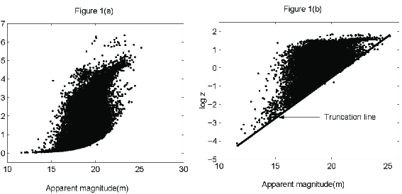
Figure 1: Apparent magnitude $(m)$ versus redshift$(z)$ in linear scale$(a)$ and in log-scale$(b)$ with truncation line, from Véron-Cetty(V-C) $(2006)$ quasar catalogue.

The magnitude limited survey employed in that catalogue points to the diagonal truncation boundary as is evident in fig.$1(b)$. The analysis clearly shows the redshift data for the range  $0<z<0.295$  fitted quite satisfactorily with a linear diagram of  $logz$  in  apparent magnitude ($m$) vs. redshift  ($z$)  diagram, agreeing well with the Hubble diagram. However, for the range  $0.3<z<\simeq 3$,  the data can be fitted with certain degree of nonlinear dependence, showing spread of redshift corresponding to a single value of apparent magnitude or vice versa.

4.1.2 Doppler Shift vs. Shifting due to Dynamic Multiple Scattering

As discussed above, the current astronomical observations point to the presence of the environment around quasars of diverse nature. So, for higher redshifts, some other mechanism should be effective and might play the dominant role compared to the Doppler mechanism. We propose the significant role of environment in our understanding of the redshift of quasars, especially through the effective evolutionary phase of their life. This can occur in the following manner :
We know

$$(1+z)=(1+z_{\rm DMS})(1+z_{\rm D})$$

which gives,

$$z=(1+z_{\rm DMS})(1+z_{\rm D})-1$$

$z_{\rm DMS}$ being the redshift due to DMS mechanism and $z_{D}$ is that due to Doppler mechanism.

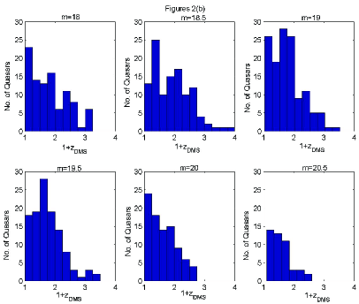
Figure 2: Relation between number of quasars and the redshift from V-C$(2006)$ quasar catalogue showing the contribution $z_{\rm DMS}$ from induced correlation mechanism(Wolf Effect) to redshift $(z)$ through the correlation parameters  $\alpha,\alpha^{\prime}$ and $\beta$  of the medium. Contribution is more prominent in the case of Radio-quiet quasars$(a)$ than that in Radio loud quasars$(b)$.

Now, let us take a particular value of $m$ and the corresponding redshift $z$ which lies on the truncation line as shown in Fig.$1(b)$ and, also, assume the $z$ values lying in the truncated line as that due to Doppler mechanism (as a rough approximation) whereas the spread in $z$ for a particular $m$ is mainly that due to the environmental effects. Then, considering that DMS active in these type of environments, we obtain from the equation(31),

$$1+z_{\rm{DMS}}=\frac{\alpha^{\prime}+(\alpha\alpha^{\prime}-\beta^{2})\delta^{2}_{N}}{|\beta|}$$ (40)

where,

$$\delta^{2}_{N}=(\frac{\beta^{2}}{{\alpha^{\prime}}^{2}})^{N}\delta_{0}^{2}+\frac{\alpha^{\prime}}{{\alpha^{\prime}}^{2}-\beta^{2}}$$

If $\delta_{0}$  is considered as due to Doppler broadening only, then

$$\delta_{N}^{2}\simeq\frac{\alpha^{\prime}}{{\alpha^{\prime}}^{2}-\beta^{2}}$$

Therefore,

$$1+z_{\rm{DMS}}=\frac{\alpha^{\prime}+(\alpha\alpha^{\prime}-\beta^{2})[\frac{\alpha^{\prime}}{{\alpha^{\prime}}^{2}-\beta^{2}}]}{|\beta|}$$ (41)

Then, what we observe as redshift, is

$$z_{obs}=\frac{\alpha^{\prime}}{\beta}\left[1+\frac{(\alpha\alpha^{\prime}-\beta^{2})}{{\alpha^{\prime}}^{2}-\beta^{2}}\right][1+z_{D}]-1$$ (42)

or,

$$1+z_{\rm obs}=\Gamma(1+z_{D})$$ (43)

where $\Gamma$  is a constant, dependent solely on the correlation parameters $\alpha,\ \alpha^{\prime},\ \beta$ of the medium through which the wave comes to the observer after experiencing multiple scattering.

The scatter plot of $m$ versus $z$ (Fig.$1(a)$)shows that there exists a set of $z$ even for a fixed $m$ i.e., a set of quasars, probably for diverse values of $\alpha,\ \alpha^{\prime},\ \beta$. Taking the values of $z$  as  $z_{\rm D}$(${\rm D}$ for Doppler)  from the truncation line(shown in Fig.$1(b)$), we find $(1+z_{\rm obs})$  from the eq.(43). Assuming a set of values for $\alpha,\ \alpha^{\prime},\beta$, and corresponding values of $\Gamma$ which can produce a certain extra redshift other than $z_{\rm D}$,  are obtained. Number of quasars vs. for a particular value of $z_{\rm D}$  has been plotted in Fig.$2(a\&b)$,  for various $m$, separately for radio quiet(Fig.2a) and radio loud quasars(Fig.2b).

We get $\Gamma\simeq 2.06$ which is solely dependent on the nature of the environment created in the laboratory condition. It is clear from the bar-diagrams(Fig. $2(a\&b)$) that there exists a sizable number of quasars around $\Gamma\simeq 2.06$ which implies that there exist large number of quasars for a particular value of $\Gamma$, indicating similar type of environments.

4.2 Effects on Distance Modulus and Line width

At this point, we can conclude that the intrinsic physical parameters of the medium (density, temperature , pressure and ionization characteristics, the effect of which are manifested through the induced correlation parameters as stated above)  through which the source radiation crosses vast astronomical distances to the point of observation, can contribute to the shifting as well as to the width of a spectral line. We can then write the relation between the width and the shift as[details in reference⁽⁸⁾]

$$W=\kappa{(\epsilon^{2}+\eta^{2}z^{2})}^{\frac{1}{2(1+z)}}$$ (44)

where $\kappa$, $\epsilon$ and $\eta$ are constants. $\kappa\epsilon=\delta_{0}^{2}$,  $\delta_{0}^{2}$  being the intrinsic spectral width of the source frequency. Taking the logarithm of both sides we can write

$$lnW=\frac{1}{2(1+z)}ln\kappa(\epsilon^{2}+\eta^{2}{z}^{2})$$ (45)

It is well known ⁽⁴⁰⁾ that the distance modulus $d$ can be written in terms of redshift $z$ as

$$d=m-M=42.38-5ln(\frac{H}{100})+5lnz+(1.086)(1-q_{0})z+O(z^{2})$$ (46)

Where $H$ is the Hubble constant in km/sec/Mpc and $M$ refers to the absolute magnitude. For small z i.e. $z<<1$ , the eq.(46) reduces to

$$d=42.38-5ln(\frac{H}{100})+\frac{1.086}{2}z\ \ \ {\rm for}\ \ \ q_{0}=\frac{1}{2}$$

This, after simplification becomes

$$z=\frac{d-C}{0.543},\ \ \ {\rm where}\ \ \ C=42.38-5ln\left(\frac{H}{100}\right)$$

Substituting this value of $z$  in eq.(45), we have

$$d=-\frac{1.086}{lnE}lnW+N\ \ \ {\rm where},\ \ \ lnE=ln(\kappa\epsilon^{2})\ \ {\rm and}\ \ \ N=C+0.543$$ (47)

The above relation(eq.47) between the distance modulus and the width has a striking similarity to the Tully-Fisher relation⁽⁴⁵⁾ but without any angular dependence. The reason is obvious since we have considered the shift and width due to scattering only, without considering any rotational effects (in other way, the angle of scattering is considered as very small i.e., $\theta\leq 15^{0}$ which is average in case of quasar). It appears that in the case of photons which are emitted almost perpendicular to the plane of the galaxy, we will be observing those photons only without any rotational effects.

4.3 Effects on Hubble Flow at High Redshift($z\geq 0.3$)

The extension of the redshift($z$) - apparent magnitude($m$) diagram towards high redshift in the Hubble diagram can be written as⁴⁶,

$$m=M-{\mathbf{K}}(z)-E(z)+5lncq_{0}^{-2}\left\{q_{0}z+(q_{0}-1)[(1+2q_{0}z)^{\frac{1}{2}}-1]\right\}+{\rm constant}$$

where $m$ is the apparent magnitude, $M$ is absolute magnitude.

$E(z)$ is a correction term due to evolution which calculates the change in the luminosity of the main sequence termination point in the Hertzsprung-Russel diagram for stars in a standard elliptical galaxy, as a function of time. However, following Sandage⁴⁷ , the value adopted here, is

$$E(z)\approx ln\left(\frac{1}{1+z}\right)$$

${\mathbf{K}(z)}$ is the ${\mathbf{K}}$-correction term which accounts for the effect of $z$, i.e., it takes into account the fact that the galaxy is no longer being observed at a particular wavelength, but at what for small redshift($z$), it would be a shorter wavelength, and also with a bandwidth term $2.5ln(1+z)$ to account for the stretching of the spectrum. Thus, ${\mathbf{K}}$ can be written as

$${\mathbf{K}}=-2.5ln(1+z)^{1-\alpha},\ \ \ \alpha=0.3$$

assuming the spectrum of quasars varies as $\nu^{-\alpha}$. Through $q_{0}$, termed the deceleration parameter, we must take into account the effects of curvature. However, there is problem considering simultaneously the effects of both the Evolution parameter and different values of $q_{0}$ which measures the departure of the linear Hubble law i.e., $m-lncz$ linear relation, generally in good arrangement for the low-redshift limit only. Following specific cosmological model i.e., with $q_{0}=1/2$ for Einstein-de Sitter model, we obtain,

$$m=M-{\mathbf{K}}(z)-E(z)+5lncz(1+z/4)+{\rm constant}\ \ \ \ \ {\rm for}\ \ \ q_{0}=1/2$$ (48)

Using eq.$(47)$ and $(48)$, the relation for apparent magnitude and absolute magnitude for standard model, i.e., $q_{0}=1/2$ can be written as

$$m=A+B+E+{\mathbf{K}}-C*D$$ (49)

where,
$A=m-M+{\rm constant}$ = $21.4$  is a constant term;
$B=\frac{5}{2.303}*lncz(1+\frac{z}{2})$  for $q_{0}=\frac{1}{2}$
$C=\frac{0.543}{(1+z)}$
$D=1+\frac{k}{2.303}*ln(1+F*z^{2})$;
$E=$  Evolution term;
${\mathbf{K}}=-\frac{2.5}{2.303}(1+z)^{1-\alpha};\ \ \ {\rm for}\ \ \ \alpha=0.3$

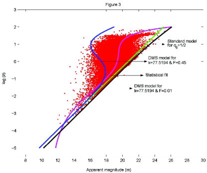
Figure 3: Comparison between Hubble curve with Standard cosmological model($q_{0}=1/2$), considering V-C$(2006)$ quasar data with that considering the proposed local environmental effects due to Induced correlation mechanism present in the medium together with statistical fitting.

$C$ and $D$ being the contributions due to the multiple scattering effect, as calculated from of induced correlation mechanism proposed in our framework, with $k=1/ln(\epsilon)$  and  $F=\eta/\epsilon$. Taking the value of $F$  and  $k$, we calculate corresponding Hubble diagram with the standard model i.e., for  $q_{0}=1/2$. But as we adopt a range of values for $F={0.45,....0.01}$,  we obtain a bulge  in Hubble diagram when approaching higher redshift limit(Fig.3). The limit of the values $k$  and $F$  as considered here, is intrinsically related to the induced correlation parameters of the medium surrounding the quasars. It is worth mentioning that, very recently, Cheng, Permutter^22,23 reviewed in detail the current situations, regarding Supernovae-redshift measurements and the corresponding Hubble diagram. They explored the possibility of having certain but variable values for cosmological parameters like $\Omega$ and the cosmological constant($\Lambda$) in order to consider the idea of accelerated expansion together with a phase transition in the evolution history of the universe and proposed an explanation of the bulging Hubble curve. Now, from eq.(45), for $z=z_{1}$,  the shift after the first scattering, is

$$z_{1}=\frac{ln\epsilon}{2\eta/\epsilon}$$

By taking, say, $F=0.5$, and $k=1/ln\epsilon\simeq 78$, the contribution in our framework from first scattering is $\sim 0.02$. It is interesting to note that the experimental values, mentioned by James and Wolf¹⁰, for $\alpha^{\prime}/\beta$  is found to range from 0.0085 to 0.146.

5 Possible Implications

The above analysis clearly indicates the following possibilities:

1. The DMS theory is applicable to a class of random media, similar to those which may be present around quasars especially as we proceed from low redshifts ($z\leq 0.295$), gradually, towards higher ranges of $z$, and this extra shift can be explained without even considering the relative motion between the observer and the source or the medium.

2. The evolutionary effect of this medium will be reflected in the DMS through a set of parameters $(\alpha,\alpha^{\prime},\beta)$  which are intrinsically related to the different physical characteristics of the media such as general dielectric susceptibility($\eta$). This, in turn is directly dependent on other physical parameters such as the refractive index($n$), permeability($\epsilon$), conductivity, temperature, pressure as well as the molecular content and degree of ionization due to the presence of the electromagnetic field.

3. However, the amount of the contribution from DMS will be dictated by the degree of the randomness or turbulence present in the medium. Here, the degree of the fluctuation of the above mentioned parameters should be such that the medium can be treated in the weak fluctuation case. We expect our mechanism to be more effective for radio quiet than for radio loud quasars (Fig. 2(a) & 2(b))where we expect suitable environment or in other words, we can describe the medium as weakly fluctuating. This information, however, will be very important, when it will be more and more available from astronomical observations(HST, KECK etc.). However, quantitative studies should be developed for this purpose with greater detail.

4. The discrepancy in the observed value of the quasars redshift should be traced back to both the Doppler as well as to the other possible local effects as reflected in DMS mechanism.

The clear deviation of the linear Hubble law for high redshift ($z$) quasars is provided in our framework for a certain range of medium parameters i.e.,  $\alpha$,  $\alpha^{\prime}$  and  $\beta$. This kind of deviation (or the existence of a bulge) has already been mentioned by several authors in connection with the Hubble diagram for high redshift Supernovae^22,23. It clearly points to the fact that there is a possibility of environmental effects on the observational aspects of quasar-like astronomical objects and their role should be considered in explaining the observed bulge and associated other criteria, i.e., the Hubble relation, especially at higher redshift in addition to the Doppler effect or gravitational redshifts. In our approach, we do not need to introduce any kind of phenomenological approaches except to consider the role played by the characteristics of the medium surrounding the radiating source. According to the currently established standard models of quasars, spectral lines are emitted from the broad line regions(BLR) as well as from the narrow line regions(NLR), i.e., from two types of clouds, named after the characteristics of lines and with respect to the position of those clouds relative to the torus surrounding the central black hole (central engine). Due to the gravitational attraction, matter from the dust torus is heated, causing it to radiate with a broad, non-thermal power spectrum. This radiation excites gaseous clouds which emit line radiation. It is worth mentioning that Wold et al.⁴⁸ have made a survey of quasar environments at $0.5\leq z\leq 0.8$ and also concluded that the quasars are located in a variety of environments, whereas, Hutchings⁽⁴⁹⁾, after his recent observations pointed out that the environment that triggers quasars activity almost certainly changes with cosmic time and with the nature and the characteristics of the emission line gas around at higher redshift quasars. Again, Papadopoulos et al.⁵⁰ reported the discovery of large amounts of low-excitation molecular gas around the infrared-luminous quasar, APM 08279+5255 at z = 3.91 and confirm the presence of an extended reservoir of molecular gas with low excitation, $10$ to $100$ times more massive than the gas traced by higher-excitation observations. This raises the possibility that significant amounts of low-excitation molecular gas may lurk in the environments of high-redshift ($z>3$) galaxies. Botoff and Ferland⁵¹ and his coworkers also point out the possible consequences about the role of turbulence and magnetic field in determining the line profiles of the emission lines which ultimately effects redshift values. Serious controversy already exists about the influence of individual quasars on their environments. It has been claimed as incontrovertible evidence for the evolution of $Ly\alpha$,  lines, especially in case of luminous quasars. From this, it appears that there is a certain kind of distribution in number density of lines and hence equivalent widths which hints to the evolution of the hydrogen column density of individual clouds of probable primordial origin, spread throughout the space. All together, it points to the essential role of the medium which is faced by the light waves that cross through the vast astronomical distance by experiencing multiple scattering in their journey. It is the nature of different physical parameters of the medium which determines ultimately the shape and nature of the spectrum we receive. This has great implications on many other aspects of astronomical observations, in scattering phenomena where the suitable physical characteristics are available for producing similar effects which we expect to study in future.

5.1 Concluding remarks

Our analysis is not complete for several reasons: At this time, we are not ready to claim adequate knowledge about the properties of the medium (such as $\alpha$,  $\alpha^{\prime}$  and  $\beta$) of the quasar environment. Also, as we are not in a position to specify quantitatively the underlying physical nature of the scattering medium, other than its anisotropic coherence properties, our model can only be considered as indicative of some possibilities. The scatterer, which is assumed to have a “white noise” power spectrum (implying that its fluctuations are very energetic and anisotropic), is situated farther away from the center of the radiating source than the line emitting clouds. These clouds can not be too hot or otherwise they would be completely ionized, making line radiation impossible. Besides these, so far we have confined our discussion to situations where the scattering medium is considered as weakly fluctuating medium and, also, if ionized, sufficiently under dense so that it can be treated as underdense plasma. Also, we have ignored the unscattered and backscattered radiation in the present problem. This effect is manifested by enhanced back scattering of light from disordered media and arises from constructive interference between propagation along forward and reverse paths. Lagendijk^52,53 noted that there is a connection between coherence-induced spectral changes and the phenomenon of weak localization. In this case, the spectral degree of coherence does not satisfy the scaling law, and, consequently, the spectrum of the backscattered radiation may be shifted relative to the spectrum of the field, very much like Wolf effect.

Acknowledgements

The authors (S.Roy and M.Roy) are greatly indebted for the kind hospitality and financial support from College of Science and Center for Earth Observation and Space Research, George Mason University, USA, during the period of this work.

References

1. Datta S., Roy S., Roy M. and Moles M.(1998), Int.Jour.Theort.Phys.,37,N5, 1469.

2. Datta S., Roy S.,Roy M. and Moles M.(1998), Phys.Rev.A,58,720.

3. Wolf E.(1986), Phys.Rev.Lett.,56,1370.

4. Wolf E.(1987),Nature,326,363.

5. Morris G.M. and Faklis D.(1987),Opt.Commun.,62,5

6. Faklis D. and Morris G.M.(1988),Opt.Lett.,13,4.

7. Wolf E.(1991),NPL Technical Bulletin:October 1991,p1

8. Roy S., Kafatos M. and Datta S.(1999), Phys.Rev.A,60, 273.

9. James D.V.F.,(1989), Phys.Lett.A.,140,213

10. James D.F.V. and Wolf E.(1990),Phy.Lett.A,146,167

11. James D. and Savedoff M.P.(1990), ApJ.,359,67.

12. Wolf E. and James D.F.V.(1996),Rep.Prog.Phys.,59,771

13. James D.F.V.(1998),Pure Appl.Opt.,7,959-970

14. Shirai T. and Asakura T.(1995),J.Opt.Soc.Am.A,12,N6,1354.

15. Shirai T. and Asakura T.(1996),Optical Rev.,3,N5,323

16. Wolf E. and Foley J.T.(1989),Phys.Rev.A,40,N2,579

17. Tatarskii V.(1998),Pure Appl.Opt.,7,953-957

18. Datta S, Roy S, Roy M and Moles M(1998),Int. Jour.Theor.Phys.,37,N4, 1313.

19. Roy S., Kafatos M. and Datta S., Astron.Astrophys.,353,1134-1138

20. Savedoff M.(1989), News l.Astronom.Soc.NY,3,22-23

21. Sulentic J.W.(1989), Astrophys.J.,343,54-65

22. Tai-Pei Cheng, http://www.umsl.edu/ tpcheng/AccUniv2/sld047.htm

23. Perlmutter S. and Schmidt Brian P., astro-ph/0303428 and references there in.

24. Wolf E.(1989), Phys Rev.Lett.,63, 2220.

25. Nussenzveig H.M.((1972), Causality and Dispersion relations(New York: Academic)

26. Watson Kenneth M.(1969), J.Math.Phys.,10,N4,688

27. Watson Kenneth M.(1970), Phys.Fluids,13,N10,2514

28. Van Hove Léon(1954), Phys.Rev.,95,N1,249;(1958),Physica,24,404

29. Glaubar R.J.(1962) in Lectures on Theoretical Physics IV(Univ. of Colorado Summer Institute for Theoretical Physics), eds. W.E.Britten,B.W.Downs and J.Downs,(Interscience,New York),p.571

30. Davenport W.B. and Root W.L.(1958),An Introduction to the Theory of Random Signals and Noise(New York:Mc-Graw-Hill)(Reprinted by IEEE Press, New York, 1987)

31. Wolf E., Foley J.T. and Gori F.(1989), Opt.Soc.Am.A,6,1142.

32. Van Cittert P.H.(1934), Physica,1,201

33. Zernike F.(1938), Physica5,785

34. Villars F. and Weisskopf V.F.(1954), Phys.Rev.,94,N2,232-240.

35. Allis W. et al.,(1963),Waves in anisotropic Plasmas(MIT Press, Cambridge),p13.

36. Born M. and Wolf E.(1998), “Principle of Optics”, 6th edition, Pergamon, Oxford.

37. Ishimaru Akira(1997) in Wave propagation and Scattering in Random Media (IEEE/OUP Series on Electromagnetic Wave Theory)

38. Ishimaru A.(1978),Wave propagation and scattering in random media, Vol II(Academic Press, New York),section 16.5.

39. Foley J.T. and Wolf E.(1989),Phys.Rev.A.,40,588

40. Gori F.,Guattari G.,Palma C.,and Padovani G.(1988) Opt.Commun,67,1

41. Efron B. and Petrosian V.,(1992), Astrophys J.,399:345-352.

42. Efron B. and Petrosian V.,(1999),Journal of the American Statistical Association,94,N447,824-834.

43. Roy S. et.al.(2006), Astro-phys/0605356, accepted for publication in Procd. of 6th International Workshop on ”Data analysis in Astronomy”, Erice, italy.

44. VERONCAT-Véron Quasars and AGNs(V2006),HEASARC Archive, ftp://cdsarc.u-strasbg.fr/pub/cats/VII/248/.

45. Tully R.B. and Fisher, J.R.(1977), A & A, 54, 661.

46. Narlikar, J. V., (1983), Introduction to Cosmology,(Jones & Bertlett Publishers,Inc.,Boston).

47. Sandage A. and Tamman G.A., (1983), in Large Scale structure of the Universe, Cosmology, and Fundamental Physics, (eds. S. setti & L. Van Hove, geneva, ESO/CERN),127

48. Wold M.,Lacy M., Lilje P.B. and Serjeant S.(2001), in ”QSO Hosts and their Environments”, QSO environments at Intermediate Redshifts and Companions at Higher Redshifts, eds. by Márquez eta al., Kluwer Academic/Plenum Publishers.

49. Hutchings John B.(2001), in”QSO Hosts and their Environments”, QSO environments at Intermediate Redshifts and Companions at Higher Redshifts, eds. by Márquez eta al., Kluwer Academic/Plenum Publishers.

50. Papadopoulos P. et al.(2001), Nature, 409, 58.

51. Botoff M. and Ferland G., Astrophys.J.(2002), 568,581-591.

52. Lagendijk A.(1990a),Phys.Lett.A,147,389.

53. Lagendijk A.(1990b),Phys.Rev.Lett.,65,2082.

Figure 1: Apparent magnitude $(m)$ versus redshift$(z)$ in linear scale$(a)$ and in log-scale$(b)$ with truncation line, from Véron-Cetty(V-C) $(2006)$ quasar catalogue.

Figure 2 : Relation between number of quasars and the redshift from V-C$(2006)$ quasar catalogue showing the contribution $z_{\rm DMS}$ from induced correlation mechanism(Wolf Effect) to redshift $(z)$ through the correlation parameters  $\alpha,\alpha^{\prime}$ and $\beta$  of the medium. Contribution is more prominent in the case of Radio-quiet quasars$(a)$ than that in Radio loud quasars$(b)$.

Figure 3: Comparison between Hubble curve with Standard cosmological model($q_{0}=1/2$), considering V-C$(2006)$ quasar data with that considering the proposed local environmental effects due to Induced correlation mechanism present in the medium together with statistical fitting.