Neutrino radiation from dense matter

Abstract

This article provides a concise review of the problem of neutrino radiation from dense matter. The subjects addressed include quantum kinetic equations for neutrino transport, collision integrals describing neutrino radiation through charged and neutral current interactions, radiation rates from pair-correlated baryonic and color superconducting quark matter.

1 Introduction

After an initial phase of rapid (of the order of weeks to years) cooling from temperatures $T\sim 50$ MeV down to 0.1 MeV, a neutron star’s core settles in a thermal quasi-equilibrium state which evolves slowly over the time scales $10^{3}-10^{4}$ yr down to temperatures $T\sim 0.01$ MeV. The cooling rate of the star during this period is determined by the processes of neutrino emission from dense matter, whereby the neutrinos, once produced, leave the star without further interactions. Understanding the cooling processes that take place during this neutrino radiation era is crucial for the interpretation of the data on surface temperatures of neutron stars. While the long term features of the thermal evolution of neutron stars are insensitive to the initial rapid cooling stage, the subsequent route in the temperature versus time diagram, which includes the late time ($t\geq 10^{5}$ yr) photoemission era, strongly depends on the emissivity of matter during the neutrino cooling era.

This lecture is a concise introduction to the physics of neutrino radiation from dense nucleonic and quark matter in compact stars. It starts with a classification of the reactions in Sec. 1.1, which is followed by a discussion of quantum kinetic equations for neutrinos and neutrino emissivities in Sec. 2. In Sec. 3 examples are given of polarization tensors of superfluid nucleonic matter and color superconducting quark matter. We close by suggesting two exercises for students.

1.1 Classification of the reactions

Historically, the weak reactions in neutron stars were classified within the quasiparticle description for fermions in matter: each reaction is distinguished by the number of the participating quasiparticles and the weak-interaction current. The simplest neutrino emission processes that involve single fermionic quasiparticle in the initial (final) state can be written as

$$f_{1}\to f_{2}+e+\bar{\nu},\quad f_{2}+e\to f_{1}+\nu,$$ (1)

$$f\to f+\nu+\bar{\nu},\hskip 142.26378pt({\rm forbidden})$$ (2)

where the first line is the charged current $\beta$-decay and its inverse, with $f_{1}$ and $f_{2}$ being neutron and proton quasiparticles in nucleonic matter or $d$ and $u$ flavor quarks in deconfined quark matter; $f$ refers to a fermion. This process is known in astrophysics as the Urca processes [1]. The Urca reaction is kinematically allowed in nucleonic matter under $\beta$-equilibrium if the proton fraction is sufficiently large, $Y_{p}\geq 11-14\%$ [2]. In deconfined, chirally symmetric, and interacting quark matter at moderate densities the Urca processes is kinematically allowed for any asymmetry between $u$ and $d$ quarks [3]. The second process - the neutral current neutrino pair bremsstrahlung, Eq. (2), is forbidden by the energy and momentum conservation, if one adopts the quasiparticle picture. If, however, we choose to work with excitations that are characterized by finite widths, the reaction (2) is allowed [4]. The processes with two fermions in the initial (and final) states are the modified Urca and its inverse [5]

$$f_{1}+f_{1}\to f_{1}+f_{2}+e+\bar{\nu},\quad f_{1}+f_{2}\to f_{2}+f_{2}+e+\bar{\nu},$$ (3)

$$f_{1}+f_{2}+e\to f_{1}+f_{1}+\nu,\quad f_{2}+f_{2}+e\to f_{2}+f_{1}+\nu,$$ (4)

and the modified bremsstrahlung process

$$f+f\to f+f+\nu+\bar{\nu}.$$ (5)

The modified processes are characterized by a spectator baryon that guarantees energy and momentum conservation in baryonic matter. In quark matter these processes are subdominant due to the extra phase space required by the spectator quarks. Indeed each extra fermion in the initial and final state introduces a small factor $T/E_{F}\ll 1$, where $E_{F}$ is the Fermi energy. The general arguments above apply to the reactions in quark matter featuring strange quarks and in the hypernuclear matter, where the kinematical constraints are less restrictive than in purely nucleonic matter [6, 7].

Due to the attractive component of the strong interaction nucleons and quarks form Cooper pairs at sufficiently low temperatures (for up-to-date reviews on nuclear and quark superconductivity see Refs. [8, 9]). The formation of Cooper condensates lifts the constraint on the neutral current one-body processes in nucleonic [10, 11] and quark matter [12], thus leading to the reaction

$$\{ff\}\to f+f+\nu_{f}+\bar{\nu}_{f},\quad f+f\to\{ff\}+\nu_{f}+\bar{\nu}_{f},$$ (6)

where $\{ff\}$ refers to a Cooper pair, $f+f$ to two quasiparticle excitations. These processes - termed Cooper pair breaking and formation (CPBF) reactions [13] - are efficient in the temperature domain $T^{*}\leq T\leq T_{c}$, where $T_{c}$ is the critical temperature of superfluid phase transition and $T^{*}\sim 0.2~{}T_{c}$; they are suppressed asymptotically at low temperatures as ${\rm exp}(-\Delta(0)/T)$, where $\Delta(0)$ is the zero-temperature pairing gap. The temperature domain above matches firmly with characteristic temperatures in the neutrino cooling era ($T_{c}\sim$ MeV for nucleonic matter). Thus, the CPBF processes are an important ingredient of the cooling of at least the nucleonic matter. The case of quark matter is less clear: the critical temperature of pairing of quarks in the dominant pairing channels could be as large as 50 MeV; however smaller, $\sim$ keV, gaps were predicted for some combinations of quantum numbers, and the associated critical temperatures lie within the relevant temperature range [9]. The neutral current processes (6) induced by the superfluidity have their charged current counterparts [14, 15]. While the former vanish, when the temperature approaches the critical temperature of superfluid phase transition, the emissivity of the latter process approaches the value of the corresponding Urca process.

2 Quantum kinetics of neutrinos in matter

Among the methods that are used to compute the rates of neutrino production in dense matter those that use the language of many-body theory are particularly suited, as the whole approach can be organized in a systematic way, that is consistent with the treatment of related problems of the equation of state, specific heat of matter, pairing fields, etc. In particular, the formulations based on the real-time Green’s functions (RTG) technique allow for treatments of non-equilibrium processes, including situations far from equilibrium. The RTG technique was applied to compute the neutrino emissivities for several reactions in nucleonic matter by Voskresensky and Senatorov [11]. In their approach the rates are computed from the $S$-matrix with the help of the optical theorem. Alternatively, the neutrino emission rates can be derived directly from a quantum kinetic equation for neutrinos, whereby the collision integrals are expressed in terms of neutrino self-energies [4, 17]. Below, the latter method will be illustrated on a few examples.

2.1 Transport equations for neutrinos

We wish to write down a transport equation for neutrinos in a general form involving only Green’s functions and self-energies. One way of doing this is to start with the Dyson equation for neutrinos written on a real time contour. At the first order in the gradient expansion, and upon taking the quasiparticle limit in neutrino propagators, one finds [17]

$$i\left\{\mathop{\rm Re}S^{-1}(q,x),S_{0}^{>,<}(q,x)\right\}_{P.B.}=S^{>,<}(q,x)\Omega^{>,<}(q,x)+\Omega^{>,<}(q,x)S^{>,<}(q,x),$$ (7)

where $S^{>,<}(q,x)$ and $\Omega^{>,<}(q,x)$ are the neutrino propagators and self-energies, $q=(q_{0},\bm{q})$ and $x=(t,\bm{x})$ are the four-momentum and space-time coordinates, $\{\dots\}_{P.B.}$ is the four-dimensional Poisson bracket; the symbols $>,<$ refer to the positioning of the time arguments of the two-point functions $S$ and $\Omega$ on the real-time contour; $\mathop{\rm Re}S^{-1}(q,x)$ is the inverse of the retarded Green’s function. The l. h. side of Eq. (7) corresponds to the drift term of the Boltzmann equation (hereafter BE), while the r. h. is the collision integral. The on-mass-shell neutrino propagator is related to the single-time distribution functions (Wigner functions) of neutrinos and anti-neutrinos, $f_{\nu}(q,x)$ and $f_{\bar{\nu}}(q,x)$, via the ansatz

$$S_{0}^{<}(q,x) = \frac{i\pi\!\not\!q}{\omega_{\nu}(\bm{q})}\Big{[}\delta\left(q_{0}-\omega_{\nu}(\bm{q})\right)f_{\nu}(q,x)-\delta\left(q_{0}+\omega_{\nu}(\bm{q})\right)\left(1-f_{\bar{\nu}}(-q,x)\right)\Big{]},$$ (8)

where $\omega_{\nu}(\bm{q})=|\bm{q}|$ is the on-mass-shell neutrino/anti-neutrino energy. Note that the ansatz includes simultaneously the neutrino particle states $\propto f_{\nu}(q,x)$ and anti-neutrino hole states $\propto 1-f_{\bar{\nu}}(-q,x)$.

Upon applying the trace operation (in the space of Dirac matrices) on both sides of the transport equation (7) and integrating out the off-shell energies on the l. h. side, one obtains a single time BE for neutrinos

$$\left[\partial_{t}+\vec{\partial}_{q}\,\omega_{\nu}(\bm{q})\vec{\partial}_{x}\right]f_{\nu}(\bm{q},x)=\int_{0}^{\infty}\frac{dq_{0}}{2\pi}{\rm Tr}\left[\Omega^{<}(q,x)S_{0}^{>}(q,x)-\Omega^{>}(q,x)S_{0}^{<}(q,x)\right];$$ (9)

a similar equation follows for the anti-neutrinos if one integrates in Eq. (7) over the range $[-\infty,0]$.

2.2 Collision integrals

Figure 1: The neutrino self-energy in the case of charged (left) and neutral (right) current interaction mediated by $W^{+}$ and $Z^{0}$ gauge bosons, respectively; the baryon/quark propagators are labeled as $f_{i}$, $i=1,2$; that of neutrino, anti-neutrino and electrons as $\nu$, $\bar{\nu}$ and $e^{-}$. Note that the $\nu$ and $\bar{\nu}$ propagators are shown for illustration and should not be included in the evaluation of the diagram.

Leading order contributions to the neutrino radiation rates arise from second order Born diagrams when the neutrino self-energies $\Omega^{>,<}(q)$ are expanded with respect to the weak coupling constant. The diagrams contributing to the charged and neutral current processes are shown in Fig. 1. The corresponding neutrino self-energies are given by

$$-i\Omega^{>,<}(q_{1},x) = \int\frac{d^{4}q}{(2\pi)^{4}}\frac{d^{4}q_{2}}{(2\pi)^{4}}(2\pi)^{4}\delta^{4}(q_{1}-q_{2}-q)i\Gamma_{q}^{\mu}\,iS_{0}^{<}(q_{2},x)i\Gamma_{q}^{\dagger\,\lambda}i\Pi^{>,<}_{\mu\lambda}(q,x),$$ (10)

where $\Pi^{>,<}_{\mu\lambda}(q)$ refer to the polarization tensors, $\Gamma_{q}^{\mu}$ is the weak interaction vertex to be specified below. The central problem of the theory is to compute the polarization tensors of nucleonic or quark matter.

To obtain the emissivity through, e. g., a charged current process, we compute from the BE the change in the energy per unit volume and time due to the change in the anti-neutrino distribution

$$\epsilon_{\bar{\nu}} = \frac{d}{dt}\int\!\frac{d^{3}q}{(2\pi)^{3}}f_{\bar{\nu}}(\bm{q})\omega_{\nu}(\bm{q})=-2\left(\frac{\tilde{G}}{\sqrt{2}}\right)^{2}\int\!\frac{d^{3}q_{1}}{(2\pi)^{3}2\omega_{e}(\bm{q}_{1})}\int\!\frac{d^{3}q_{2}}{(2\pi)^{3}2\omega_{\nu}(\bm{q}_{2})}\int\!d^{4}q\,\delta(\bm{q}_{1}+\bm{q}_{2}-\bm{q})$$ (11)

$$\delta(\omega_{e}+\omega_{\nu}-q_{0})\,\omega_{\nu}(\bm{q}_{2})g_{B}(q_{0})\left[1-f_{\bar{\nu}}(\omega_{\bar{\nu}})\right]\left[1-f_{e}(\omega_{e})\right]\Lambda^{\mu\zeta}(q_{1},q_{2})\mathop{\rm Im}\,\Pi^{R}_{\mu\zeta}(q),$$

where $\tilde{G}=G{\rm cos~{}}\theta_{C}$, $G$ is the weak coupling constant, $\theta_{C}$ is the Cabibbo angle (${\rm cos~{}}\theta_{C}=0.973$) and $\Lambda^{\mu\zeta}(q_{1},q_{2})={\rm Tr}\left[\gamma^{\mu}(1-\gamma^{5})\!\not\!q_{1}\gamma^{\zeta}(1-\gamma^{5})\!\not\!q_{2}\right]$. The symbol $\mathop{\rm Im}$ refers to the imaginary part of the polarization tensor’s resolvent. Here we used the relation $\Pi_{\mu\zeta}^{<}(q)=\Pi_{\zeta\mu}^{>}(-q)=2ig_{B}(q_{0}){\mathop{\rm Im}}\,\Pi_{\mu\zeta}^{R}(q)$, where $g_{B}(q_{0})$ is the Bose distribution function and $\Pi^{R}_{\mu\zeta}(q)$ is the retarded component of the polarization tensor. In equilibrium, $f_{\bar{\nu}/e}(\omega_{\bar{\nu}/e})$ reduce to Fermi-distribution functions for anti-neutrinos and electrons. Since the anti-neutrinos leave the star without interactions, there is no thermal population of anti-neutrinos, i. e. $f_{\bar{\nu}}(\omega_{\bar{\nu}})\ll 1$ and can be neglected. The neutrino emissivity for the case of neutral current processes can be obtained in a similar way [4, 17].

3 Polarization tensors of dense matter: Examples

It is instructive to study the polarization tensors describing charged and neutral current processes first at the single loop level. Descriptions that are consistent with the conservation laws and Ward identities require vertex corrections to the one-loop results, which we shall address later on. We shall now switch to the equilibrium finite temperature techniques of Matsubara Green’s functions thus treating the nucleonic/quark matter in thermal equilibrium.

3.1 Direct Urca process in baryonic matter

Since the temperature of dense matter core during the neutrino cooling era is well below the critical temperatures of pairing in baryonic and quark matter, pairing correlations should be included in the computation of polarization tensors. The non-relativistic Matsubara propagators that incorporate the pairing correlations are given by

$$\hat{G}^{M}_{\alpha\alpha^{\prime}}(ip_{n},\bm{p}) = \delta_{\sigma\sigma^{\prime}}\delta_{\tau\tau^{\prime}}\left(\frac{u_{p}^{2}}{ip_{n}-\varepsilon_{p}}+\frac{v_{p}^{2}}{ip_{n}+\varepsilon_{p}}\right)=\delta_{\sigma\sigma^{\prime}}\delta_{\tau\tau^{\prime}}G^{M}(ip_{n},\bm{p}),$$ (12)

$$\hat{F}_{\alpha\alpha^{\prime}}(ip_{n},\bm{p}) = -i\sigma_{y}\delta_{\tau\tau^{\prime}}u_{p}v_{p}\left(\frac{1}{ip_{n}-\varepsilon_{p}}-\frac{1}{ip_{n}+\varepsilon_{p}}\right),$$ (13)

where $p_{n}=(2n+1)\pi T$ is the fermionic Matsubara frequency, $\sigma$ and $\tau$ refer to spin and isospin, $\sigma_{y}$ is the $y$-component of the Pauli-matrix, $u_{p}^{2}=(1/2)(1+\xi_{p}/\varepsilon_{p})$ and $v_{p}^{2}=1-u_{p}^{2}$ are the Bogolyubov amplitudes and $\varepsilon_{p}=\sqrt{\xi_{p}^{2}+\Delta_{p}^{2}}$ is the quasiparticle spectrum, where $\xi_{p}=p^{2}/2m^{*}-\mu$ is the spectrum in the unpaired state, with $m^{*}$ and $\mu$ being the effective mass and chemical potential. Here $\Delta_{p}$ is the anomalous self-energy (gap function). The propagators above are written for the case of $S$-wave neutron or proton proton pairing in isospin-1, spin-0 state. Note that at high densities the neutron fluid is paired in a $P$ wave (this is not the case for protons because of their low abundance). Consider now the case of direct Urca process involving nucleons (Fig. 1, left diagram). The Matsubara polarization tensor is then given by

$$i\Pi_{\mu\nu}^{M}(iq,\bm{q})=\sum_{ip}\int\frac{d^{3}p}{(2\pi)^{3}}{\rm Tr}\left[\Gamma_{\mu}G_{\tau=1/2}^{M}(ip,\bm{p})\Gamma_{\nu}G_{\tau=-1/2}^{M}(ip+iq,\bm{p}+\bm{q})\right],$$ (14)

where the charged current weak interaction vertices are $\Gamma_{\mu}=\gamma_{\mu}(1-g_{A}\gamma^{5})$, with $g_{A}=1.26$ being the axial coupling constant. Upon performing the Matsubara sums and analytical continuation $(iq\to\omega+i\delta)$ we obtain the retarded polarization tensor

$$\Pi_{V/A}^{R}(iq,\bm{q}) = 2\int\frac{d^{3}p}{(2\pi)^{3}}\Biggl{\{}\left(\frac{u_{p}^{2}u_{p+q}^{2}}{\omega+\varepsilon_{p}-\varepsilon_{p+q}+i\delta}-\frac{v_{p}^{2}v_{p+q}^{2}}{\omega-\varepsilon_{p}+\varepsilon_{p+q}+i\delta}\right)\left[f(\varepsilon_{p})-f(\varepsilon_{p+q})\right]$$ (15)

$$+u_{p}^{2}v_{p+q}^{2}\left(\frac{1}{\omega-\varepsilon_{p}-\varepsilon_{p+q}+i\delta}-\frac{1}{\omega+\varepsilon_{p}+\varepsilon_{p+q}+i\delta}\right)\left[1-f(\varepsilon_{p})-f(\varepsilon_{p+q})\right]\Biggr{\}},$$

where the vector/axial-vector polarization tensors $\Pi^{R}_{V/A}$ are the components proportional to $1$ and $g_{A}^{2}$, respectively. The first two terms in Eq. (15) correspond to excitations of a particle-hole pair while the last two to excitation of particle-particle and hole-hole pairs. The last term does not contribute to the neutrino radiation rate $(\omega>0)$. We identify the first two terms as the scattering ($SC$) terms, while the third term as the pair-braking ($PB$) term. Upon evaluating the phase space integrals, the neutrino emissivity is written as $\epsilon_{\bar{\nu}}=\epsilon_{0}^{\rm Urca}J,$ where

$$\epsilon_{0}^{\rm Urca}=(1+3g_{A}^{2})\frac{3\tilde{G}^{2}m_{n}^{*}m_{p}^{*}p_{Fe}T^{6}}{2\pi^{5}},\quad J=-\frac{1}{6}\int_{-\infty}^{\infty}\!dy~{}g_{B}(y)\left[I^{SC}(y)+I^{PB}(y)\right]\int_{0}^{\infty}dzz^{3}f_{e}(z-y),$$ (16)

where $p_{Fe}$ is the Fermi-momentum of the electrons and $y=\beta\omega$; the integrals $I^{SC}(y)$ and $I^{PB}(y)$ are given in Refs. [14]. In the unpaired state ($u_{p}\to 1$ and $v_{p}\to 0$) only the scattering contribution survives; upon integrating we obtain

$$I^{SC}(y)={\rm ln}\Bigg{|}\frac{1+{\rm exp}\left[-\beta\xi\right]}{1+{\rm exp}\left[-\beta(\xi+\omega)\right]}\Bigg{|},$$ (17)

where $\xi=\tilde{p}^{2}/2m^{*}-\mu_{p}$ and $\tilde{p}=(m^{*}/q)(\omega-\mu_{p}+\mu_{n}-q^{2}/2m^{*})$; here the momentum transfer $q=p_{Fe}$, $\mu_{n}$ and $\mu_{p}$ are the chemical potentials of neutrons and protons, and we assumed for simplicity that their effective masses are equal. In the zero temperature limit $I^{SC}(y)=y\theta(-\beta\xi)$, the integrals in Eq. (16) can be performed analytically and one recovers the zero-temperature result of Lattimer et al. [2]. The zero temperature $\theta$-function can be rewritten as $\theta(p_{Fe}+p_{Fp}-p_{Fn})$ [2] which tells us that the “triangle inequality” $p_{Fe}+p_{Fp}\geq p_{Fn}$ must be obeyed by the Fermi-momenta of the particles for the Urca process to operate.

While the one-loop approximation provides a useful starting point, the complete treatment of the problem when the particle-hole interaction is not small, i. e. can not be treated as a perturbation, requires summation of infinite series of particle-hole loops. This is certainly the case in nuclear matter, where the Landau parameters are $O(1)$.

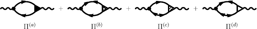
Figure 2: The sum of polarization tensors that contribute to the neutrino emission rate. The single arrowed solid line corresponds to the normal propagator (12), while the double arrowed line to the anomalous propagator (13). The contributions form $\Pi^{(b)}(q)$, $\Pi^{(c)}(q)$, and $\Pi^{(d)}(q)$ diagrams vanish at one-loop for the Urca process; the $\Pi^{(d)}(q)$ diagram is finite for charge neutral interactions at one-loop.

Figure 2 shows the four distinct diagrams in the case where the loops are summed up to all orders. Next subsection shows how to improve on the one-loop result using as an example the neutral current interactions.

3.2 Neutral current neutrino pair-bremsstrahlung

The polarization tensor describing the neutral current interactions in baryonic matter is given by

$$i\Pi_{\mu\nu}(q)=\sum_{ip}\int\frac{d^{3}p}{(2\pi)^{3}}{\rm Tr}\left[\Gamma_{\nu}G(ip,\bm{p})\Gamma_{\mu}G(ip+iq,\bm{p}+\bm{q})+\Gamma_{\nu}\hat{F}(ip,\bm{p})\Gamma_{\mu}\hat{F}^{\dagger}(ip+iq,\bm{p}+\bm{q})\right],$$ (18)

where the neutral current vertices are $\Gamma_{\mu}=\gamma_{\mu}(c_{V}-c_{A}\gamma^{5})$. Performing the Matsubara sums we obtain for the vector and axial-vector contributions in this case

$$\Pi^{V/A}(q) = \sum_{\sigma\bm{p}}\left[f(\varepsilon_{p})-f(\varepsilon_{k})\right]\left(\frac{A_{\mp}}{iq+\varepsilon_{p}-\varepsilon_{k}}-\frac{B_{\mp}}{iq-\varepsilon_{p}+\varepsilon_{k}}\right)$$ (19)

$$+ \sum_{\sigma\bm{p}}\left[f(-\varepsilon_{p})-f(\varepsilon_{k})\right]\left(\frac{C_{\mp}}{iq-\varepsilon_{k}-\varepsilon_{p}}-\frac{D_{\mp}}{iq+\varepsilon_{p}+\varepsilon_{k}}\right),$$

where $k=p+q$, $A_{\mp}=u_{p}^{2}u_{k}^{2}\mp h$, $B_{\mp}=v_{p}^{2}v_{k}^{2}\mp h$, $C_{\mp}=u_{k}^{2}v_{p}^{2}\pm h$, $D_{\mp}=u_{p}^{2}v_{k}^{2}\pm h$, $h=u_{p}u_{k}v_{p}v_{k}$. The first line in Eq. (19) corresponds to the process of scattering where a quasiparticle is promoted out of the condensate into an excited state, or inversely, an excitation merges with the condensate. The corresponding piece of the response function $\mathop{\rm Im}\Pi^{V/A}(q)$ vanishes for small momentum transfers. The second line in Eq. (19) describes the process of pair-breaking and recombination, i. e., excitation of pairs of quasiparticles out of the condensate, and inversely, restoration of a pair within the condensate. Since we are interested in the emission process we shall keep only the terms that do not vanish for $\omega>0$; then, the pair-braking contribution is given by the term $\propto C_{\pm}$. This contribution to the polarization tensor can be evaluated analytically in the limit $\bm{q}\to 0$ and the case $\Delta\neq\Delta(p)$ and is given by

$$\mathop{\rm Im}\,\Pi^{V}(q) = -2\pi\nu(p_{F})g(\omega)^{-1}f\left(\frac{\omega}{2}\right)^{2}\left(\frac{\Delta^{2}}{\omega^{2}}\right)\frac{\omega}{\sqrt{\omega^{2}-4\Delta^{2}}}\theta(\omega-2\Delta),$$ (20)

$$\mathop{\rm Im}\,\Pi^{A}(q) \simeq 0+O\left(\frac{v_{F}^{2}}{c^{2}}\right),$$ (21)

where $\nu(p_{F})=m^{*}p_{F}/2\pi^{2}$ is the density of states ($\hbar=1$) and $\theta$ is the Heaviside step function; the explicit form of the $O\left({v_{F}^{2}}/{c^{2}}\right)$ contribution to the axial current response is given by Flowers et al in Ref. [10].

Upon substituting Eq. (20) in the neutral current analog of Eq. (11) and carrying out the phase-space integrals we obtain the emissivity per neutrino flavor [10]

$$\epsilon_{\nu\bar{\nu}}=\frac{G^{2}\,c_{V}^{2}}{240\pi^{3}}~{}~{}\nu(p_{F})~{}T^{7}~{}I_{1}(\zeta)\equiv\epsilon_{0}^{\rm brems.}~{}I_{1}(\zeta),$$ (22)

where $\zeta=2\Delta(T)/T$ and

$$I_{1}(\zeta)=\zeta^{7}\int_{0}^{\infty}\!\!d\phi~{}({\rm cosh}\,\phi)^{5}~{}f\left(\frac{\zeta}{2}\,{\rm cosh}\,\phi\right)^{2}.$$ (23)

Note that the rate (22) scales as $\zeta^{7}$ and, consequently, it is sensitive to the magnitude of the pairing gap. Because of the substantial density dependence of the gap, the emissivity (22) varies strongly across the stellar interior.

In nuclear and neutron matter problem the particle-hole interactions are not small and cannot be treated in the perturbation theory. The resummation of particle-hole diagrams in a superfluid leads to coupled integral equations shown in Fig. 3. In the non-relativistic limit the driving terms in the vector and axial-vector channels correspond to the scalar and spinor perturbations, i. e. the bare vector and axial-vector vertices are $\Gamma^{V}=1$ and $\Gamma^{A}=\bm{\sigma}$. The topologically non-equivalent polarization tensors and the associated vertices are shown in Figs. 2 and  3.

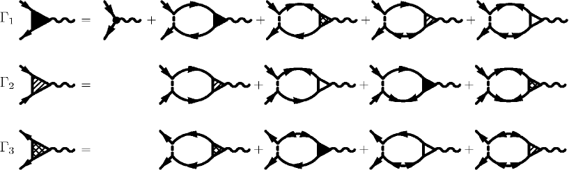
Figure 3: Coupled integral equations for the effective weak vertices in superfluid baryonic matter. The “normal” $\Gamma_{1}$ vertex (full triangle) and two “anomalous” vertices $\Gamma_{2}$ (hatched) and $\Gamma_{3}$ (shaded triangle) are shown explicitly, the fourth vertex (empty triangle) is obtained by interchanging the particle and hole lines in the first line. The anomalous vertices vanish in the normal state.

Including the vertex corrections modifies the one-loop result to (Sedrakian et al. in ref. [10])

$$\epsilon_{\nu\bar{\nu}}=\epsilon_{0}~{}(I_{2}+I_{3}),$$ (24)

where

$$I_{2} = -\frac{1}{\pi\nu(p_{F})T^{7}}\int_{0}^{\infty}\!\!d\omega~{}\omega^{6}g(\omega)\sum_{i=1}^{3}\left[{\rm Im}\Pi_{i}(\omega)~{}{\rm Re}\Gamma_{i}(\omega)\right],$$ (25)

$$I_{3} = -\frac{1}{\pi\nu(p_{F})T^{7}}\int_{0}^{\infty}\!\!d\omega~{}\omega^{6}g(\omega)\sum_{i=1}^{3}\left[{\rm Re}\Pi_{i}(\omega)~{}{\rm Im}\Gamma_{i}(\omega)\right],$$ (26)

where $\Pi_{1}=\Pi^{(a)}-\Pi^{(d)}$, $\Pi_{2}=\Pi^{(b)}$ and $\Pi_{3}=\Pi^{(c)}$. For $T\to T_{c}$ the rates vanish, consistent with the observation that the pair bremsstrahlung is absent in normal matter for on-shell (non-interacting) baryons. At small $T\leq 0.3T_{c}$ the rates are suppressed exponentially as ${\rm exp}(-\Delta/T)$.

3.3 Direct Urca process in color superconducting matter

Although quark matter in compact stars and its superfluidity were suggested more than three decades ago, these topics have received much attention in recent years after the models, which were designed to describe the chiral phase transition in dense matter, were applied to the problem of quark superconductivity (the current state of the art is reflected in the reviews [9]). At moderate densities relevant to compact stars the quark matter is in the non-perturbative regime and one has to rely on effective models that capture (at least some) features predicted by the QCD (chiral symmetry breaking, confinement, etc.) The ground state of superconducting quark matter under $\beta$-equilibrium is not known; one significant problem is that under the stress caused by $\beta$-equilibrium and/or the strange quark mass, the Fermi-surfaces of up ($u$) and down ($d$) quarks are shifted apart, and the resulting pairing patterns differ from the ones predicted by the BCS theory. Color and flavor degrees of freedom are responsible for the multitude of possible pairing patterns.

In contrast to the case of nucleonic matter the Urca process is permitted in interacting quark matter for any asymmetry between $u$ and $d$ quarks. The emissivity to first order in the strong coupling constant $\alpha_{c}$ is given by [3]

$$\epsilon_{0}=\frac{914}{315}~{}\tilde{G}_{F}^{2}~{}\alpha_{c}~{}\mu_{d}~{}\mu_{u}~{}\mu_{e}~{}T^{6},$$ (27)

where $\mu_{i}$, $i=d,\,u,\,e\,$ are the chemical potentials of down and up quarks and electrons. If non-superconducting quark matter is present in the core of a neutron star, the star will cool very rapidly to temperatures well below the observational threshold.

What are the effects of superfluidity on the cooling rate of such a star? Let us consider a specific model [15], where the pairing is in the so-called 2SC phase, i. e. quark pairing is characterized by the order parameter $\Delta\propto\langle\psi^{T}(x)C\gamma_{5}\tau_{2}\lambda_{2}\psi(x)\rangle$, where $\tau_{2}$ is the Pauli matrix in the isospin state, $\lambda_{2}$ is the Gell-Mann matrix in the color space, $C=i\gamma^{2}\gamma^{0}$ is the matrix of charge conjugation. The minimal effective Lagrangian describing the pairing is given by

$${\cal L}_{\rm eff}=\bar{\psi}(x)(i\gamma^{\mu}\partial_{\mu})\psi(x)+G_{1}(\psi^{T}C\gamma_{5}\tau_{2}\lambda_{A}\psi(x))^{\dagger}(\psi^{T}C\gamma_{5}\tau_{2}\lambda_{A}\psi(x)),$$ (28)

where $G_{1}$ is the attractive pairing interaction. The Lagrangian is minimal in the sense that apart from the pairing interaction it includes only the kinetic term for massless quarks; other channels of interaction, such as the repulsive components which would lead to the renormalizations of the single-particle spectra of quarks are omitted. The normal and anomalous propagators of quarks of flavor $f$ are

$$S_{f=u,d}=i\delta_{ab}\frac{\Lambda^{+}(p)}{(p_{0}+\delta\mu)^{2}-\varepsilon_{p}^{2}}(\!\not\!p-\mu_{f}\gamma_{0}),\quad\quad F(p)=-i\epsilon_{ab3}\epsilon_{fg}\Delta\frac{\Lambda^{+}(p)}{(p_{0}+\delta\mu)^{2}-\varepsilon_{p}^{2}}\gamma_{5}C,$$ (29)

where $\varepsilon_{p}=\sqrt{(p-\mu)^{2}+\Delta^{2}}$, $\delta\mu=(\mu_{d}-\mu_{u})/2$ and $\mu=(\mu_{d}+\mu_{u})/2$, $\Lambda^{+}$ is the projector to the positive energy state. The emissivity at one-loop can be obtained by evaluating the sum

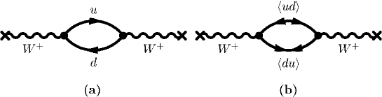
Figure 4: One-loop $W$-polarization tensor: (a) normal piece, which represents the sole contribution above $T_{c}$; and (b) “anomalous” piece, which is proportional to $\Delta^{2}(T)$ and vanishes at $T_{c}$.

of diagrams in Fig. 4, which leads to the polarization tensor

$$\Pi_{\mu\lambda}(q)=-i\int\frac{d^{4}p}{(2\pi)^{4}}{\rm Tr}\left[(\Gamma_{-})_{\mu}S(p)(\Gamma_{+})_{\lambda}S(p+q)+(\Gamma_{-})_{\mu}F(p)(\Gamma_{+})_{\lambda}F(p+q)\right],$$ (30)

where $\Gamma_{\pm}(q)=\tilde{G}\gamma_{\mu}(1-\gamma_{5})\otimes\tau_{\pm}$ and $\tau_{\pm}=(\tau_{1}\pm\tau_{2})/2$ are flavor-raising and lowering operators. The result for the emissivity depends on whether the parameter $\zeta=\Delta/\delta\mu$ is larger or smaller than unity [15]. For $\zeta>1$ all the particle modes are “gapped”, therefore, as the temperature is lowered, the emissivity is suppressed (for asymptotically low temperatures exponentially). When $\zeta<1$ there are gapless modes in the quasiparticle spectrum; this implies that the neutrino production is not affected by color superconductivity for these modes. As a result, the superconducting quark matter cools at a rate comparable to the unpaired matter. Fig. 5 illustrates these two distinct cases.

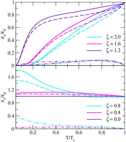
Figure 5: Temperature dependence of the neutrino emissivity normalized to its value at the critical temperature for a range of values of $\zeta=\Delta(0)/\delta\mu$; the upper panel corresponds to the gapped regime ($\zeta>1$) while the lower panel to the gapless regime ($\zeta<1$). The dashed and dashed-dotted lines are the normal and anomalous contributions; the solid line is their sum.

The neutrino emissivity of color-superconducting matter has been studied for alternative realizations of the ground state matter: one such realization is the spin-1 color superconductivity [16]. Since the condensate in this case breaks the rotational symmetry the neutrino emission turns out to be anisotropic for some choices of the order parameter [18]. Another realization is the crystalline color superconductivity, which is characterized by spatially modulated gap parameter. The neutrino radiation rates from crystalline color superconducting matter and cooling of compact stars featuring such a phase is discussed in Refs. [19].

4 Suggested exercises

1. Derive the emissivity of the direct Urca process $n\to p+e+\bar{\nu}$ in unpaired matter by using the Fermi Golden rule and following the similar derivation of the emissivity of the modified Urca process $n+n\to n+p+e+\bar{\nu}$ in Ref. [20]. Rederive the emissivity in unpaired matter by setting $u_{p}=1$ and $v_{p}=0$ in Eq. (15) and $\Lambda^{\mu\lambda}{\rm Im}\Pi^{R}_{\mu\lambda}\simeq 8\omega_{e}\omega_{\nu}({\rm Im}\Pi_{V}+3g_{A}^{2}{\rm Im}\Pi_{A})$ in Eq. (11).

2. Derive the emissivity of unpaired quark matter featuring $u$ and $d$ quarks through the direct Urca process $d\to u+e+\bar{\nu}$ by using the Fermi Gold rule in the case where the quarks interact to leading order in $\alpha_{s}$ [3]. Repeat the calculation by starting from the polarization tensor (30) with $\Delta=0$ (see Ref. [15] for the case $\Delta\neq 0$). Next assume that quarks are non-interacting but massive. Repeat the calculations in this case and compare to the result of Ref. [3].

References

- [1] G. Gamow and M. Schoenberg, Phys. Rev. 59, 539 (1941); C. J. Pethick, Rev. Mod. Phys. 64, 1133 (1992).
- [2] J. Boguta, Phys. Lett. B 106, 255 (1981); J. M. Lattimer, C. J. Pethick, M. Prakash, and P. Haensel, Phys. Rev. Lett. 66, 2701 (1991).
- [3] N. Iwamoto, Phys. Rev. Lett. 44, 1637 (1980); A. Burrows, ibid. 1640.
- [4] A. Sedrakian and A. Dieperink, Phys. Lett. B 463, 145 (1999); see also J. Knoll and D. N. Voskresensky, Ann. Phys. 249, 532 (1996).
- [5] H. Y. Chiu and E. E. Salpeter, Phys. Rev. Lett. 12, 413 (1964); J. N. Bahcall and R. A. Wolf, Phys. Rev. Lett. 14, 343 (1965); Phys. Rev. 140, B145 (1965).
- [6] R. C. Duncan, I. Wasserman, and S. L. Shapiro, ApJ 278, 806 (1984).
- [7] M. Prakash, M. Prakash, C. J. Pethick, and J. M. Lattimer, ApJ 390, L77 (1992).
- [8] A. Sedrakian and J. W. Clark, eprint nucl-th/0607028.
- [9] M. G. Alford, eprint hep-lat/0610046; M. Alford and K. Rajagopal, eprint hep-ph/0606157; M. Alford, Prog. Theor. Phys. Suppl. 153, 1 (2004); D. Blaschke, nucl-th/0603063; M. Buballa, Phys. Rep. 407, 205 (2005); G. Nardulli, epirnt hep-ph/0610285; D. H. Rischke, Prog. Part. Nucl. Phys. 52, 197 (2004); S. B. Rüster et al., eprint nucl-th/0602018. T. Schaefer, eprint nucl-th/0602067.
- [10] E. G. Flowers, M. Ruderman, and P. G. Sutherland, Astrophys. J. 205, 541 (1976); A. D. Kaminker, P. Haensel, and D. G. Yakovlev, Astron. Astrophys. 345, L14 (1999); L. B. Leinson, Nucl. Phys. A 687, 489 (2001); A. Sedrakian, H. Müther and P. Schuck, eprint nucl-th/0611676.
- [11] D. N. Voskresensky and A. V. Senatorov, Sov. J. Nucl. Phys. 45, 411 (1987) [Yad. Fiz. 45, 657 (1987)].
- [12] P. Jaikumar and M. Prakash, Phys. Lett. B 516, 345 (2001).
- [13] C. Schaab, D. N. Voskresensky, A. Sedrakian, F. Weber, and M. Weigel, Astron. Astrophys. 321, 591 (1996).
- [14] A. Sedrakian, Phys. Lett. B 607, 27 (2005); Prog. Part. Nucl. Phys. 58, 168 (2007), eprint nucl-th/0601086.
- [15] P. Jaikumar, C. D. Roberts, and A. Sedrakian, Phys. Rev. C 73, 042801(R) (2006).
- [16] T. Schaefer, Phys. Rev. D 62, 094007 (2000); M. G. Alford, J. A. Bowers, J. M. Cheyne, and G. A. Cowan, Phys. Rev. D 67, 054018 (2003); D. N. Aguilera, D. Blaschke, H. Grigorian, N. N. Scoccola, Phys. Rev. D 74, 114005 (2006); D. N. Aguilera, D. Blaschke, M. Buballa, V. L. Yudichev, Phys. Rev. D 72, 034008 (2005); A. Schmitt, Phys. Rev. D 71, 054016 (2005).
- [17] A. Sedrakian and A. Dieperink, Phys. Rev. D 62, 083002 (2000).
- [18] A. Schmitt, I. A. Shovkovy, and Q. Wang, Phys. Rev. D 73, 034012 (2006); Q. Wang, Zhi-Gang Wang, Jian Wu, Phys. Rev. D 74 014021.
- [19] R. Anglani, G. Nardulli, M. Ruggieri, and M. Mannarelli, Phys. Rev. D 74, 074005 (2006); R. Anglani, eprint hep-ph/0610404.
- [20] S. L. Shapiro and S. A. Tuekolsky, Black Holes, White Dwarfs and Neutron Stars: The Physics of Compact Objects (John Willey & Sons, New York, 1983).