Gravitational instability on the brane: the role of boundary conditions

Abstract

An outstanding issue in braneworld theory concerns the setting up of proper boundary conditions for the brane–bulk system. Boundary conditions (BC’s) employing regulatory branes or demanding that the bulk metric be nonsingular have yet to be implemented in full generality. In this paper, we take a different route and specify boundary conditions directly on the brane thereby arriving at a local and closed system of equations (on the brane). We consider a one-parameter family of boundary conditions involving the anisotropic stress of the projection of the bulk Weyl tensor on the brane and derive an exact system of equations describing scalar cosmological perturbations on a generic braneworld with induced gravity. Depending upon our choice of boundary conditions, perturbations on the brane either grow moderately (region of stability) or rapidly (instability). In the instability region, the evolution of perturbations usually depends upon the scale: small scale perturbations grow much more rapidly than those on larger scales. This instability is caused by a peculiar gravitational interaction between dark radiation and matter on the brane. Generalizing the boundary conditions obtained by Koyama and Maartens, we find for the Dvali–Gabadadze–Porrati model an instability, which leads to a dramatic scale-dependence of the evolution of density perturbations in matter and dark radiation. A different set of BC’s, however, leads to a more moderate and scale-independent growth of perturbations. For the mimicry braneworld, which expands like LCDM, this class of BC’s can lead to an earlier epoch of structure formation.

1 Introduction

A specific feature of braneworld models of gravity [1, 2] and cosmology [3, 4, 5] is that the arena of observable events occurs in a lower-dimensional Lorentzian submanifold of the higher-dimensional space-time. For instance, in the scenario which we shall be considering, the brane is a four-dimensional boundary of a space-time with a noncompact (‘infinite’) extra dimension, and an observer is in direct contact only with the induced metric on the brane. In this situation, one might worry about the well-posedness of physical problems from the observer’s viewpoint. Indeed, phenomena taking place on the brane can depend upon physical conditions in the higher-dimensional bulk manifold which is inaccessible to an observer living on the brane. Consequently, the brane observer loses the ability of predicting classical physical phenomena on the brane. Indeed, it appears that no initial-value problem can be well posed on the brane since, no matter how detailed the specification of the initial conditions on a spacelike hypersurface on the brane, this does not uniquely determine events occurring either in the future or the past of this hypersurface. At best, one can uniquely predict the events in the future of a Cauchy hypersurface on the brane if one has the knowledge of the entire past to this hypersurface (and vice versa). This situation is illustrated by Fig. 1, which depicts the brane as a boundary of a bulk space with a noncompact extra dimension. Let a solution of the bulk–brane system be given. By smoothly perturbing data on a hypersurface $S$ in the bulk at some distance from the brane, one modifies the solution on the brane only to the past of the hypersurface $A$ and to the future of the hypersurface $B$; hence, even complete knowledge of the data on the brane in the region between the hypersurfaces $A$ and $B$ is not sufficient for predicting the evolution to the past or future of this region. This is sometimes expressed by saying that the braneworld equations are nonlocal from the viewpoint of an observer living on the brane.

Figure 1: Brane as a four-dimensional boundary of the five-dimensional bulk.
By smoothly perturbing the data on a hypersurface $S$ in the bulk at some distance from the brane, one modifies the solution on the brane only to the past of the hypersurface $A$ and to the future of the hypersurface $B$; hence, even complete knowledge of the data on the brane in the spacetime region between the hypersurfaces $A$ and $B$ is not sufficient for predicting the evolution to the past or future of this region.

One might try to limit the space of solutions by specifying some appropriate boundary conditions for the full brane–bulk system. Much effort has been applied to formulate reasonable conditions in the bulk, by demanding that the bulk metric be nonsingular or by employing other (regulatory) branes. However, to date, these proposals have not been implemented in the braneworld theory in full generality — with certain success they were used only in a linearized theory under some additional approximations (see e.g., [6, 7, 8]) — and it is clear that such an approach to boundary conditions still leaves intact the property of nonlocality described above.

The issue of cosmological perturbations on the brane in induced-gravity models remains poorly studied in the literature precisely because of the difficulties posed by the nonlocal character of this theory and the lack of proper boundary conditions. Thus, in treating the scalar perturbations on the brane, one is led to consider the problem in the bulk space using, for instance, the Mukohyama master variable [9], which is a scalar function describing gravitational degrees of freedom in the bulk and obeying there a second-order partial differential equation. The corresponding initial-value problem was argued to be well posed in the brane–bulk system [10]. However, in this case, one needs to specify initial conditions on the brane as well as in the bulk, with the obvious complication of having to deal with a function dependent on the coordinate of the extra dimension. This problem can be tackled to some extent in the linear approximation, but looks insurmountable when nonlinearities in the metric become significant — and, in principle, they can become significant in the bulk space much ‘earlier’ than on the brane. And — what is more important — one still has to face the problem of boundary conditions in the bulk, since not all possible values of the Mukohyama variable may lead to well-behaved solutions of the brane-bulk system.

In an earlier paper [11], we suggested a new approach to the issue of boundary conditions for the brane–bulk system. From a broader perspective, boundary conditions can be regarded as any conditions which restrict the space of solutions. Our idea was to specify such conditions directly on the brane which represents the observable world, so as to arrive at a local and closed system of equations on the brane. In fact, this is what some researches usually do in practice in the form of making various reasonable assumptions (see, e.g., [12, 13] for the issue of cosmological perturbations; and [14] for the case of spherically symmetric solutions on the brane). The behaviour of the metric in the bulk is of no further concern in this approach, since this metric is, for all practical purposes, unobservable directly. As first noted in [15], the nonlocality of the braneworld equations is connected with the dynamical properties of the bulk Weyl tensor projected on to the brane. It therefore seems logical to impose certain restrictions on this tensor in order to obtain a closed system of equations on the brane.

Neglecting the projected Weyl tensor on the brane [16], though simple, is incorrect [7] since it is incompatible with the equation that follows from the Bianchi identity [see Eq. (9) below]. Hence, to proceed along this road, one needs to impose some other condition on this tensor. Perhaps, the simplest choice is to set to zero its (appropriately defined) anisotropic stress. This condition is fully compatible with all equations of the theory and eventually amounts to a brane universe described by a modified theory of gravity with an additional invisible component — the Weyl fluid, or dark radiation — having nontrivial dynamics. However, this is not a unique prescription and we shall discuss other possibilities in this paper applying some of them to the study of scalar cosmological perturbations on the brane.

An important result of this paper is that our choice of boundary conditions (BC’s) strongly influences the growth of density perturbations. For a class of BC’s, a qualitative analysis of the linearized equations for scalar perturbations in a matter-dominated braneworld reveals the existence of an instability. In particular, the boundary condition which formally coincides with the approximate condition derived in [7] in the context of the Dvali–Gabadadze–Porrati (DGP) model [2], leads to a dramatic dependence of the growth of perturbations on spatial scale. In a matter-dominated braneworld, perturbations on small spatial scales grow many orders of magnitude larger than those on large spatial scales, indicating an early breakdown of linear regime. The cause of this instability is a peculiar gravitational interaction between matter and dark radiation on the brane which arises for this class of BC’s. Our qualitative conclusions are supported by a numerical integration of the exact system of linearized equations. A different choice of BC’s, however, leads to a perfectly ‘normal’ situation in which the growth of perturbations is moderate and virtually independent of scale.

In the DGP model, the brane tension and the bulk cosmological constant are both set to zero, and the current acceleration of the universe expansion is explained as an effect of extra dimension without severe fine tuning of the fundamental constants of the theory. However, an interesting situation arises also in the opposite case, where both these constants are large. As shown in [11], a low-density braneworld exactly mimics the expansion properties of the LCDM model. In particular, a universe consisting solely of baryons with $\Omega_{\rm b}\simeq 0.04$ can mimic the LCDM cosmology with a much larger ‘effective’ value of the matter density $\Omega_{\rm m}\simeq 0.2$$-$$0.3$. A conventional low-density universe runs into trouble with observations on account of its slow growth rate of perturbations. It is therefore interesting that such a model survives in the braneworld context which allows perturbations to grow much faster.

Whether one can altogether do away with the notion of dark matter, as suggested in [17, 18] is a moot point, since, in addition to alleviating the so-called growth problem, dark matter also explains other observations including rotation curves of galaxies, etc. Whether all such observations can be accommodated in induced-gravity models is an interesting open subject which we set aside for future investigations. For recent results in frames of the the induced-gravity models, see our paper [19].

This paper is organized as follows: In section 2, we introduce the theory and formulate the boundary conditions. In section 3, we apply the theory to the issue of scalar cosmological perturbations. We derive an exact convenient system of equation governing the growth of perturbations of pressureless matter and dark radiation and discuss boundary conditions of various type. In section 4, we study numerically the evolution of perturbations in the DGP cosmology, and in section 5 we do this for the mimicry braneworld models. Finally, we discuss our results in section 6.

2 Boundary conditions for the brane–bulk system

We consider a generic braneworld model with the action given by the expression

$$M^{3}\left[\int_{\rm bulk}\left({\cal R}-2\Lambda\right)-2\int_{\rm brane}K\right]+\int_{\rm brane}\left(m^{2}R-2\sigma\right)+\int_{\rm brane}L\left(h_{ab},\phi\right)\,.$$ (1)

Here, ${\cal R}$ is the scalar curvature of the metric $g_{ab}$ in the five-dimensional bulk, and $R$ is the scalar curvature of the induced metric $h_{ab}=g_{ab}-n_{a}n_{b}$ on the brane, where $n^{a}$ is the vector field of the inner unit normal to the brane, which is assumed to be a boundary of the bulk space, and the notation and conventions of [20] are used. The quantity $K=h^{ab}K_{ab}$ is the trace of the symmetric tensor of extrinsic curvature $K_{ab}=h^{c}{}_{a}\nabla_{c}n_{b}$ of the brane. The symbol $L(h_{ab},\phi)$ denotes the Lagrangian density of the four-dimensional matter fields $\phi$ whose dynamics is restricted to the brane so that they interact only with the induced metric $h_{ab}$. All integrations over the bulk and brane are taken with the corresponding natural volume elements. The symbols $M$ and $m$ denote the five-dimensional and four-dimensional Planck masses, respectively, $\Lambda$ is the bulk cosmological constant, and $\sigma$ is the brane tension. Note that the Hilbert–Einstein term $\int_{\rm brane}m^{2}R$ may be induced by quantum fluctuations of matter fields residing on the brane [2, 4]. This idea was originally suggested by Sakharov in the context of his induced gravity model of general relativity [21].

The following famous cosmologies are related to important subclasses of action (1):

1. The Randall–Sundrum model [1] is obtained after setting $m=0$ in (1).

2. The Dvali–Gabadadze–Porrati model [2] corresponds to the special case where both the cosmological constant in the bulk and the brane tension vanish, i.e., $\Lambda=0$ and $\sigma=0$ in (1).

3. Finally, general relativity, leading to the LCDM cosmological model, is obtained after setting $M=0$ in (1).

In addition to the above, braneworld cosmology described by (1) is very rich in possibilities and leads to several new and interesting cosmological scenarios including the following [11, 22, 23, 24]:

• Braneworld universe can accelerate at late times, and the effective equation of state of dark energy can be $w_{\rm eff}\leq-1$ as well as $w_{\rm eff}\geq-1$. The former provides an example of phantom cosmology without the latter’s afflictions.

• The current acceleration of the universe is a transient feature in a class of braneworld models. In such models, both the past and the future are described by matter-dominated expansion.

• The braneworld scenario is flexible enough to allow a spatially flat universe to loiter in the past ($z\geq\mbox{few}$). During loitering, the universe expands more slowly than in LCDM (i.e., $H(z)/H_{\rm LCDM}<1$), which leads to interesting observational possibilities for this scenario.

• For large values of some of its parameters, the braneworld can mimic LCDM at low redshifts, so that $H(z)\simeq H_{\rm LCDM}$ and $w_{\rm eff}\simeq-1$ for $z\leq\mbox{few}$. At higher redshifts, the Hubble parameter departs from its value in concordance cosmology leading to important observational possibilities.

It is therefore quite clear that the action (1) can give rise to cosmological models with quite definite attributes and properties. Confronting these models against observations becomes a challenging and meaningful exercise. At present, most tests of these models have been conducted under the assumption that the three-dimensional brane is homogeneous and isotropic [25]. Since braneworld cosmology has passed these tests successfully, the next step clearly is to probe it deeper by examining its perturbations. This shall form the focus of the present paper.

The action (1) leads to the Einstein equation with cosmological constant in the bulk:

$${\cal G}_{ab}+\Lambda g_{ab}=0\,,$$ (2)

while the field equation on the brane is

$$m^{2}G_{ab}+\sigma h_{ab}=T_{ab}+M^{3}\left(K_{ab}-h_{ab}K\right)\,,$$ (3)

where $T_{ab}$ is the stress–energy tensor on the brane stemming from the last term in action (1). By using the Gauss–Codazzi identities and projecting the field equations onto the brane, one obtains the effective equation [11, 15]

$$G_{ab}+\Lambda_{\rm eff}h_{ab}=8\pi G_{\rm eff}T_{ab}+{1\over\beta+1}\left({1\over M^{6}}Q_{ab}-C_{ab}\right)\,,$$ (4)

where

$$\beta={2\sigma m^{2}\over 3M^{6}}$$ (5)

is a dimensionless parameter,

$$\Lambda_{\rm eff}={1\over\beta+1}\left({\Lambda\over 2}+{\sigma^{2}\over 3M^{6}}\right)$$ (6)

is the effective cosmological constant,

$$8\pi G_{\rm eff}={\beta\over\beta+1}\cdot{1\over m^{2}}$$ (7)

is the effective gravitational constant,

$$Q_{ab}=\frac{1}{3}EE_{ab}-E_{ac}E^{c}{}_{b}+\frac{1}{2}\left(E_{cd}E^{cd}-\frac{1}{3}E^{2}\right)h_{ab}$$ (8)

is a quadratic expression with respect to the ‘bare’ Einstein equation $E_{ab}\equiv m^{2}G_{ab}-T_{ab}$ on the brane, and $E=h^{ab}E_{ab}$. The symmetric traceless tensor $C_{ab}\equiv n^{c}n^{d}C_{acbd}$ in (4) is a projection of the bulk Weyl tensor $C_{abcd}$. It is connected with the tensor $Q_{ab}$ through the equation following from the energy conservation and Bianchi identity:

$$\widetilde{\nabla}^{a}\left(Q_{ab}-M^{6}C_{ab}\right)=0\,,$$ (9)

where $\widetilde{\nabla}^{a}$ denotes the covariant derivative on the brane associated with the induced metric $h_{ab}$.

The system of equations (2), (3) can have many formal solutions — too many to represent physically admissible cases. The issue that arises is what conditions should determine the space of its physical solutions. A common approach consists in demanding that the bulk space be singularity free. This approach is physically most appealing; however, because of obvious difficulties, it is very difficult to implement this idea in practice. (In the Appendix, we critically discuss the recent efforts [7, 8] to derive the proper boundary condition in this way.) Moreover, it may not be really necessary to impose this condition given that the entire observable world is represented by the brane only. Provided that the physical situation on the brane is regular, it may not be vital to worry about the situation in the bulk. This last consideration suggests that one might try to impose boundary conditions for the brane–bulk system not far away in the bulk but closer to home — directly on the brane or in a close neighbourhood of the brane — since this approach is likely to be the one most relevant for an observer residing in our (3+1)-dimensional universe.

It is clear that the absence of the time derivatives of certain components of the traceless symmetric tensor $C_{ab}$ in Eq. (9) results in a functional arbitrariness in the dynamics of this tensor on the brane. Hence, it is reasonable to postulate boundary conditions in the form of certain constraints imposed on this tensor. In fact, conditions of this sort on the components of the tensor $C_{ab}$ have been applied in many papers as an approximation or a reasonable guess (see, e.g., [12, 13] for a discussion in the Randall–Sundrum model). Here, we would like to consider such conditions as an exact physical principle.

The tensor $C_{ab}$ can be decomposed through a convenient physically determined normalized timelike vector field $u^{a}$ on the brane (see [12]):

$$m^{2}C_{ab}=\rho_{\cal C}\left(u_{a}u_{b}+\frac{1}{3}q_{ab}\right)+2v_{(a}u_{b)}+\pi_{ab}\,,$$ (10)

where

$$q_{ab}=h_{ab}+u_{a}u_{b}$$ (11)

is the tensor of projection to the tangent subspace orthogonal to $u^{a}$, and the covector $v_{a}$ and traceless symmetric tensor $\pi_{ab}$ are both orthogonal to $u^{a}$. In this decomposition, the quantities $\rho_{\cal C}$, $v_{a}$, and $\pi_{ab}$ have the meaning of dark-radiation density, momentum transfer, and anisotropic stress, respectively, as measured by observers following the world lines tangent to $u^{a}$.

The anisotropic stress can be further conveniently decomposed into scalar, vector, and tensor parts in the following way:

$$\pi_{ab}=\left[D_{(a}D_{b)}-\frac{1}{3}q_{ab}D^{2}\right]\pi_{\cal C}+D_{(a}\pi_{b)}+\widetilde{\pi}_{ab}\,.$$ (12)

Here, we have introduced the derivative operator $D_{a}$ acting on tensor fields $T^{cd\cdots}_{ef\cdots}$ tangent to the brane and orthogonal to $u^{a}$ according to the rule

$$D_{a}T^{cd\cdots}_{ef\cdots}=\prod\widetilde{\nabla}_{a}T^{cd\cdots}_{ef\cdots}\,,$$ (13)

where the symbol $\prod$ denotes the projection using $q_{ab}$ with respect to all tensorial indices. For example,

$$D_{a}\pi_{b}=q^{c}{}_{a}q^{d}{}_{b}\widetilde{\nabla}_{c}\pi_{d}\,.$$ (14)

If the vector field $u^{a}$ is hypersurface orthogonal, then $q_{ab}$ represents the induced metric in the family of hypersurfaces orthogonal to $u^{a}$, and $D_{a}$ is the (unique) derivative operator on these hypersurfaces compatible with this induced metric. Furthermore, the covector field $\pi_{a}$ and the symmetric tensor $\widetilde{\pi}_{ab}$ in (12) are both orthogonal to $u^{a}$ and, for their unique specification, the latter can also be assumed to have zero trace and ‘spatial divergence’ (i.e., to be trace-free and ‘transverse’):

$$h^{ab}\widetilde{\pi}_{ab}=0\,,\qquad D^{a}\widetilde{\pi}_{ab}=0\,.$$ (15)

The first of these conditions implies $D^{a}\pi_{a}=0$.

There are no evolution equations for the tensor fields $\pi_{ab}$ on the brane, which is a manifestation of the nonlocality problem discussed in the introduction. Therefore, boundary conditions on the brane can be specified by imposing additional conditions on this tensor. The simplest possible choice of such conditions would be to set it entirely to zero:

$$\pi_{ab}=0\,.$$ (16)

In this case, equation (9) gives the evolution equations for the remaining dark-radiation components $\rho_{\cal C}$ and $v_{a}$. However, other conditions on the components $\pi_{\cal C}$, $\pi_{a}$, and $\widetilde{\pi}_{ab}$ of the anisotropic stress are possible. Without introducing any additional dimensional parameters into the theory, one can relate the scalar ‘spatial Laplacian’ $D^{2}\pi_{\cal C}$ to the energy density $\rho_{\cal C}$

$$D^{2}\pi_{\cal C}=A\rho_{\cal C}\,,$$ (17)

while setting $\pi_{a}=0$ and $\widetilde{\pi}_{ab}=0$. Here, $A$ is some dimensionless covariant scalar. In this paper, we mostly assume $A$ to be just a constant so that the boundary condition (17) forms a one-parameter family.

Boundary conditions of the type (16) or (17) clearly depend on the choice of the timelike vector field $u^{a}$ used in the decompositions (10) and (12). In order for these BC’s to be covariantly specified, the vector field $u^{a}$ should be determined by the intrinsic geometric properties of the brane. One can think of several options as to the choice of this field. For example, one can identify $u^{a}$ with a timelike eigenvector (thereby demanding the existence of such an eigenvector) of a geometric quantity such as $C^{a}{}_{b}$, $R^{a}{}_{b}$, $K^{a}{}_{b}$, etc. We will not attempt to make a specific prescription in this paper. In studying cosmological scalar perturbations, it will be sufficient to assume that the unperturbed field $u^{a}$ is tangent to the world lines of isotropic observers — the only distinguished choice — and that it is perturbed linearly. In this case, condition (17) represents a generalization of the approximate boundary condition derived in [7, 8] for the DGP cosmology [2, 5] (there, the value $A=-1/2$ was obtained).

The specific form (16) or (17) of our set of boundary conditions, of course, contains some arbitrariness. To us it seems to be the simplest one of the kind of boundary conditions that we propose (specified directly on the brane); however, we cannot justify its uniqueness at this moment. Therefore, it should be regarded as a proposal which demonstrates how the braneworld theory with our type of boundary conditions can operate in principle, and which can be tested observationally. Perhaps, one should keep in mind that the specific form of boundary conditions in the multi-dimensional space is part of any braneworld theory with large extra dimension, to be tested against observations.

After the boundary conditions have been specified, the tensor $C_{ab}$ plays the role of the stress–energy tensor of an ideal fluid with equation of state like that of radiation but with a nontrivial dynamics described by Eq. (9). In the literature, this tensor has been called ‘Weyl fluid’ [26] and, in the cosmological context, ‘dark radiation’ [27]. The stress–energy of this ideal fluid is not conserved due to the presence of the source term $Q_{ab}$ in (9). Equation (4) together with boundary conditions such as those described by (10)–(17) form a complete set of equations on the brane.

3 Scalar cosmological perturbations

3.1 Main equations

The unperturbed metric on the brane is described by the Robertson–Walker line element and brane expansion is described by [4, 5, 22]

$$H^{2}+{\kappa\over a^{2}}={\rho+\sigma\over 3m^{2}}+{2\over\ell^{2}}\left[1\pm\sqrt{1+\ell^{2}\left({\rho+\sigma\over 3m^{2}}-{\Lambda\over 6}-{C\over a^{4}}\right)}\right]\,,$$ (18)

where $\rho$ is the matter density,

$$\ell={2m^{2}\over M^{3}}$$ (19)

defines a new fundamental length scale, $\kappa=0,\pm 1$ describe different possibilities for the spatial geometry and the term $C/a^{4}$ ($C$ is a constant) is the homogeneous contribution from dark radiation. The two signs in (18) describe two different branches corresponding to the two different ways in which a brane can be embedded in the Schwarzschild–anti-de Sitter bulk [4, 5]. In [22], we classified models with lower (upper) sign as Brane 1 (Brane 2). Models with the upper sign can also be called self-accelerating because they lead to late-time cosmic acceleration even in the case of zero brane tension and bulk cosmological constant [5]. Throughout this paper, we consider the spatially flat case ($\kappa=0$) for simplicity.

On a spatially homogeneous and isotropic brane, the timelike vector field $u^{a}$ used in the decomposition (10) coincides with the four-velocity field of isotropic observers comoving with matter, and the homogeneous dark-radiation density $\rho_{\cal C}$ is related to the constant $C$ by $\rho_{\cal C}=-3m^{2}C/a^{4}$. Due to spatial homogeneity and isotropy, we have $\pi_{a}=0$ and $\pi_{ab}=0$, and equation (17) then implies $\rho_{\cal C}=0\ \Rightarrow\ C=0$ (for $A\neq 0$).

Scalar metric perturbations are most conveniently described by the relativistic potentials $\Phi$ and $\Psi$ in the so-called longitudinal gauge:

$$ds^{2}=-(1+2\Phi)dt^{2}+a^{2}(1-2\Psi)d\vec{x}^{2}\,.$$ (20)

We denote the components of the linearly perturbed stress–energy tensor of matter in the coordinate basis as follows:

$$T^{\alpha}{}_{\beta}=\left(\begin{array}[]{rl}\displaystyle-(\rho+\delta\rho)\,,&\displaystyle-\partial_{i}v\vskip 6.0pt plus 2.0pt minus 2.0pt\\ \displaystyle{\partial_{i}v\over a^{2}}\,,&\displaystyle(p+\delta p)\delta^{i}{}_{j}\end{array}\right)\,,$$ (21)

where $\delta\rho$, $\delta p$, and $v$ are small quantities. Similarly, we introduce the scalar perturbations $\delta\rho_{\cal C}$, $v_{\cal C}$, and $\delta\pi_{\cal C}$ of the tensor $C_{ab}$ in the coordinate basis:

$$m^{2}C^{\alpha}{}_{\beta}=\left(\begin{array}[]{rl}\displaystyle{3m^{2}C\over a^{4}}-\delta\rho_{\cal C}\,,&\displaystyle-\partial_{i}v_{\cal C}\vskip 6.0pt plus 2.0pt minus 2.0pt\\ \displaystyle{\partial_{i}v_{\cal C}\over a^{2}}\,,&\displaystyle\left({\delta\rho_{\cal C}\over 3}-{m^{2}C\over a^{4}}\right)\delta^{i}{}_{j}+{\delta\pi^{i}{}_{j}\over a^{2}}\end{array}\right)\,,$$ (22)

where, according to (12), $\delta\pi_{ij}=\partial_{i}\partial_{j}\delta\pi_{\cal C}-\frac{1}{3}\delta_{ij}\partial^{2}\delta\pi_{\cal C}$, and the spatial indices are raised and lowered with $\delta^{i}{}_{j}$. We call $v$ and $v_{\cal C}$ the momentum potentials for matter and dark radiation, respectively.

Then, equation (4) together with the stress–energy conservation equation for matter and conservation equation (9) for dark radiation result in the following complete system of equations describing the evolution of scalar perturbations on the brane:

$$\displaystyle\ddot{\Psi}+3(1+\gamma)H\dot{\Psi}+H\dot{\Phi}+\left[2\dot{H}+3H^{2}(1+\gamma)\right]\Phi-{\gamma\over a^{2}}\nabla^{2}\Psi+{1\over 3a^{2}}\nabla^{2}(\Phi-\Psi)$$

$$=\displaystyle\left[c_{s}^{2}-\gamma+{2\over\ell^{2}\lambda}\left(c_{s}^{2}-\frac{1}{3}\right)\right]{\delta\rho\over 2m^{2}}+\left(1+{2\over\ell^{2}\lambda}\right){\tau\delta S\over 2m^{2}}\,,$$ (23)

$$\delta\dot{\rho}+3H(\delta\rho+\delta p)=3(\rho+p)\dot{\Psi}+{1\over a^{2}}\nabla^{2}v\,,$$ (24)

$$\dot{v}+3Hv=\delta p+(\rho+p)\Phi\,,$$ (25)

$$\delta\dot{\rho}_{\cal C}+4H\delta\rho_{\cal C}={1\over a^{2}}\nabla^{2}v_{\cal C}-{12m^{2}C\over a^{4}}\dot{\Psi}\,,\vskip 6.0pt plus 2.0pt minus 2.0pt$$ (26)

$$\dot{v}_{\cal C}+3Hv_{\cal C}=\frac{1}{3}\delta\rho_{\cal C}-{4m^{2}C\over a^{4}}\Phi-{m^{2}\ell^{2}\dot{\lambda}\over 3H}\left[{\Delta_{\rm m}\over 2m^{2}}-{\nabla^{2}\over a^{2}}\Psi\right]-{m^{2}\ell^{2}\lambda\over 3a^{2}}\nabla^{2}(\Phi-\Psi)\,,$$ (27)

$${1\over a^{2}}\nabla^{2}\Psi=\left(1+{2\over\ell^{2}\lambda}\right){\Delta_{\rm m}\over 2m^{2}}+{\Delta_{\cal C}\over m^{2}\ell^{2}\lambda}\,,$$ (28)

$$m^{2}\ell^{2}\lambda\left(\dot{\Psi}+H\Phi\right)=\left(1+{\ell^{2}\lambda\over 2}\right)v+v_{\cal C}\,,$$ (29)

$$\delta\pi_{\cal C}=-{m^{2}\ell^{2}\lambda\over 4}\left(1+3\gamma\right)(\Phi-\Psi)\,.$$ (30)

Here, we use the following notation: $S$ is the entropy density of the matter content of the universe, $\tau=\left(\partial p/\partial S\right)_{\rho}\,$, $c_{s}^{2}=\left(\partial p/\partial\rho\right)_{S}$ is the adiabatic sound velocity, the time-dependent functions $\lambda$ and $\gamma$ are given by

$$\lambda\equiv H^{2}-{\rho+\sigma\over 3m^{2}}-{2\over\ell^{2}}=\pm{2\over\ell^{2}}\sqrt{1+\ell^{2}\left({\rho+\sigma\over 3m^{2}}-{\Lambda\over 6}-{C\over a^{4}}\right)}\,,$$ (31)

$$\gamma\equiv\displaystyle\frac{1}{3}\left(1+{\dot{\lambda}\over H\lambda}\right)=\frac{1}{3}\left[1-{\displaystyle{\rho+p\over m^{2}}-{4C\over a^{4}}\over\displaystyle 2\left({\rho+\sigma\over 3m^{2}}+{1\over\ell^{2}}-{\Lambda\over 6}-{C\over a^{4}}\right)}\right]\,,$$ (32)

and the perturbations $\Delta_{\rm m}$ and $\Delta_{\cal C}$ are defined as

$$\Delta_{\rm m}=\delta\rho+3Hv\,,\qquad\Delta_{\cal C}=\delta\rho_{\cal C}+3Hv_{\cal C}\,.$$ (33)

The overdot, as usual, denotes the partial derivative with respect to the time $t$.

The system of equations (23)–(30) generalizes the work of Deffayet [10] (for the DGP brane) to the case of a generic braneworld scenario described by (1), which allows non-zero values for the brane tension and bulk cosmological constant. It describes two dynamically coupled fluids: matter and dark radiation. It is important to emphasize that the evolution equations (26), (27) for the dark-radiation component are not quite the same as those for ordinary radiation. Of special importance are the last two source terms on the right-hand side of (27) which lead to nonconservation of the dark-radiation density. Thus, the behaviour of this component is rather nontrivial, as will be demonstrated in the next section.

It is also interesting to note that the perturbations in dark radiation formally decouple from those in ordinary matter in the important limiting case $M\to 0$ (equivalently, $\ell\to\infty$), for which the system (23)–(30) reproduces the corresponding equations of general relativity (after setting $\gamma=c_{s}^{2}$).

From equations (24)–(29), one can derive the following useful system for perturbations in pressureless matter and dark radiation in the important case $C=0$ :

$$\ddot{\Delta}+2H\dot{\Delta}=\left(1+{6\gamma\over\ell^{2}\lambda}\right){\rho\Delta\over 2m^{2}}+(1+3\gamma){\delta\rho_{\cal C}\over m^{2}\ell^{2}\lambda}\,,$$ (34)

$$\dot{v}_{\cal C}+4Hv_{\cal C}=\gamma\Delta_{\cal C}+\left(\gamma-\frac{1}{3}\right)\Delta_{\rm m}+{4\over 3(1+3\gamma)a^{2}}\nabla^{2}\delta\pi_{\cal C}\,,$$ (35)

$$\delta\dot{\rho}_{\cal C}+4H\delta\rho_{\cal C}={1\over a^{2}}\nabla^{2}v_{\cal C}\,,$$ (36)

where

$$\Delta\equiv{\Delta_{\rm m}\over\rho}$$ (37)

is the conventional dimensionless variable describing matter perturbations.

3.2 Boundary conditions

The system of equations (23)–(30), or (34)–(36), describing scalar cosmological perturbations, is not closed on the brane since the quantity $\delta\pi_{\cal C}$ in (30) or (35) (hence, the difference $\Phi-\Psi$) is undetermined and, in principle, can be set arbitrarily from the brane viewpoint. This is a particular case of the nonclosure of the basic equations of the braneworld theory which we noted earlier. As discussed in the introduction, our approach to this issue will be different from that in other papers in that we will not look to the bulk to specify boundary conditions but, rather, will specify such conditions directly on the brane.

A general family of boundary conditions on the brane is obtained by relating the quantities $\pi_{\cal C}$ and $\rho_{\cal C}$ as discussed in the introduction. Equation (17) implies $C=0$ in the case $A\neq 0$ and, in the linearized form, becomes

$${1\over a^{2}}\nabla^{2}\delta\pi_{\cal C}=A\,\delta\rho_{\cal C}\,.$$ (38)

In most of this paper, $A$ shall be assumed to be a constant. By virtue of (30), this relates the difference $\Phi-\Psi$ between the gravitational potentials to the perturbation of the dark-radiation density $\delta\rho_{\cal C}$ :

$${1\over a^{2}}\nabla^{2}(\Phi-\Psi)=-{4A\over m^{2}\ell^{2}\lambda(1+3\gamma)}\delta\rho_{\cal C}\,.$$ (39)

For the boundary condition (38), one can derive a second-order differential equation for $\delta\rho_{\cal C}$ by substituting for $v_{\cal C}$ from (36) into (35):

$$\delta\ddot{\rho}_{\cal C}+(10-\gamma)H\delta\dot{\rho}_{\cal C}+4\left[\dot{H}+3(2-\gamma)H^{2}\right]\delta\rho_{\cal C}$$

$$={1\over a^{2}}\nabla^{2}\left[\gamma\delta\rho_{\cal C}+{4A\over 3(1+3\gamma)}\delta\rho_{\cal C}+\left(\gamma-\frac{1}{3}\right)\Delta_{\rm m}\right]\,.$$ (40)

Equations (34) and (3.2) will then form a closed system of two coupled second-order differential equations for $\Delta$ and $\delta\rho_{\cal C}$. From the form of the right-hand side of (3.2) one expects this system to have regions of stability as well as instability. Specifically, a necessary condition for stability on small spatial scales is that the sign of the coefficient of $\nabla^{2}\delta\rho_{\cal C}$ on the right-hand side of (3.2) be positive. This leads to the condition

$$A\geq-\frac{3}{4}\gamma(1+3\gamma)\,.$$ (41)

From (32), we find that $\gamma\approx-1/6$ in a matter-dominated universe, and condition (41) simplifies to

$$A\geq\frac{1}{16}\,.$$ (42)

We consider two important subclasses of (38) which we call the minimal boundary condition and the Koyama–Maartens boundary condition, respectively:

3.2.1 Minimal boundary condition.

Our simplest condition (16) corresponds to setting $A=0$. Then, from (30) we obtain the relation $\Phi=\Psi$, the same as in general relativity. Under this condition, equations (23)–(25) constitute a complete system of equations for scalar cosmological perturbations on the brane in which initial conditions for the relativistic potential $\Phi$, $\dot{\Phi}$ and matter perturbations $\delta\rho$, $\delta p$, $v$ can be specified quite independently. Once a solution of this system is given, one can calculate all components of dark-radiation perturbations using (28) and (29). Thus, with this boundary condition, equations (26)–(29) can be regarded as auxiliary and can be used to felicitate and elucidate the dynamics described by the main system (23)–(25). We should stress that only the quantities pertaining to the induced metric on the brane ($\Phi$, $\Psi$) and those pertaining to matter ($\delta\rho$, $\delta p$, $v$) can be regarded as directly observable, while those describing dark radiation ($\delta\rho_{\cal C}$, $v_{\cal C}$) are not directly observable.

3.2.2 Koyama–Maartens boundary condition.

In an important paper [7], Koyama and Maartens arrived at condition (38) with

$$A=-\frac{1}{2}\,.$$ (43)

This boundary condition was derived in [7] as an approximate relation in the DGP model valid only on small (subhorizon) spatial scales under the assumption of quasi-static behaviour. It was later re-derived in [8] under a similar approximation. However, according to the approach to boundary conditions taken in the present paper, one can regard (43) as being a linearized version of the more general relation (17) which is valid on all spatial scales. We call it the Koyama–Maartens boundary condition, although one should be aware of the different status of this relation in our paper, where it is regarded as an exact additional relation, and in [7, 8], where it is derived as an approximation to the more complicated situation.

In discussing the small-scale approximation in quasi-static regime, it was argued in [7] that equation (36) permits one to neglect the perturbation $v_{\cal C}$ in (35), which, together with (38), will then transform (34) into a closed equation for matter perturbations:

$$\ddot{\Delta}+2H\dot{\Delta}=\Theta_{\rm KM}\,{\rho\Delta\over 2m^{2}}\,,\qquad\Theta_{\rm KM}=1+{12A\gamma+3\gamma+1\over\ell^{2}\lambda\left[2A+\frac{3}{2}\gamma(1+3\gamma)\right]}\,.$$ (44)

Some cosmological consequences of this approach are discussed in [28]. As in general relativity, this equation does not contain spatial derivatives; hence, the evolution of $\Delta$ is independent of the spatial scale. We would obtain equation of the type (44) for perturbations had we followed the route of [7] or [8] in finding approximate solutions of perturbation equations in the bulk and using the quasi-static approximation (some difficulties with this approach are discussed in the appendix). However, in the approach adopted in this paper, as will be shown in the following two sections, numerical integration of the exact linearized system (34)–(36) does not support approximation (44). No matter what initial conditions for dark radiation are set initially, one observes a strong dependence of the evolution of matter perturbations on the wave number. In particular, it is incorrect to neglect the quantity $v_{\cal C}$ on small spatial scales, since it is precisely this quantity which is responsible for the dramatic growth of perturbations both in $\Delta_{\rm m}$ and in $\delta\rho_{\cal C}$ on such scales.

From equations (41) and (42), we can see that the minimal and Koyama–Maartens boundary conditions generally lead to unstable evolution. This will be confirmed by numerical simulations in the next section.

3.2.3 Scale-free boundary conditions.

Evolution of perturbations in the stability region (41) & (42) shows little dependence on spatial scale. It is interesting that there also exists an important class of boundary conditions leading to exact scale-independence. We call these, for simplicity, scale-free boundary conditions. To remove the dependence on wave number altogether and thereby obtain a theory in which perturbations in matter qualitatively evolve as in standard (post-recombination) cosmology, it suffices to set the right-hand side of (35) identically zero:

$${1\over a^{2}}\nabla^{2}\delta\pi_{\cal C}={1+3\gamma\over 4}\Bigl{[}(1-3\gamma)\Delta_{\rm m}-3\gamma\Delta_{\cal C}\Bigr{]}\,,$$ (45)

which, in view of equation (28), can also be expressed in a form containing only the geometrical quantities $\delta\pi_{\cal C}$, $\Delta_{\cal C}$, and $\Psi$. In this case, the perturbations $\delta v_{\cal C}$ and $\delta\rho_{\cal C}$ in dark radiation decay very rapidly, according to equations (35) and (36), and (34) reduces to the simple equation

$$\ddot{\Delta}+2H\dot{\Delta}=\Theta\,{\rho\Delta\over 2m^{2}}\,,\qquad\Theta=\left(1+{6\gamma\over\ell^{2}\lambda}\right)\,,$$ (46)

valid on all spatial scales. Equations (28) and (30) then lead to simple relations between the gravitational potentials $\Phi$ and $\Psi$ and matter perturbations:

$${1\over a^{2}}\nabla^{2}\Phi=\Theta{\Delta_{\rm m}\over 2m^{2}}\,,\qquad{1\over a^{2}}\nabla^{2}\Psi=\left(1+{2\over\ell^{2}\lambda}\right){\Delta_{\rm m}\over 2m^{2}}\,.$$ (47)

The difference $\Phi-\Psi$ can be conveniently determined from

$${1\over a^{2}}\nabla^{2}(\Phi-\Psi)={3\gamma-1\over m^{2}\ell^{2}\lambda}\Delta_{\rm m}\,.$$ (48)

As can easily be seen from (30) or (48), the general-relativistic relation $\Phi=\Psi$ is not usually valid in braneworld models. An important exception to this rule is provided by the mimicry models discussed in section 5.3.

One can propose other conditions of type (45) that lead to scale-independent behaviour. For instance, one can equate to zero the right-hand side of (3.2). But it remains unclear how these may be generalized to the fully nonlinear case as was done in the case of the boundary conditions (38) via equation (17). Nevertheless, in view of the interesting properties of scale-independence and the fact that perturbations in the stability region (41) & (42) behave in this manner, the consequences of (46) need to be further explored, and we shall return to this important issue later on in this paper.

Having described the system of linearized equations governing the evolution of scalar perturbations in pressureless matter and dark radiation, we now proceed to apply them to two important braneworld models: the popular DGP model [2, 5] and the ‘mimicry’ model suggested in [11]. It should be noted that these two models are complementary in the sense that the mimicry model arises for large values of the bulk cosmological constant $\Lambda$ and brane tension $\sigma$, whereas the DGP cosmology corresponds to the opposite situation $\Lambda=0$ and $\sigma=0$.

4 Scalar perturbations in the DGP model

Amongst alternatives to LCDM, the Dvali–Gabadadze–Porrati (DGP) model [2] stands out because of its stark simplicity. Like the cosmological constant which features in LCDM, the DGP model too has an extra parameter $\ell={2m^{2}/M^{3}}$, the length scale beyond which gravity effectively becomes five-dimensional. However, unlike the cosmological constant whose value must be extremely small in order to satisfy observations, the value $\ell\sim cH_{0}^{-1}$, required to explain cosmic acceleration, can be obtained by a ‘reasonable’ value of the five-dimensional Planck mass $M\sim 10$ MeV. As pointed out earlier, DGP cosmology belongs to the class of induced gravity models which we examine and is obtained from (1) after setting to zero the brane tension and the cosmological constant in the bulk (i.e., $\sigma=0$ and $\Lambda=0$). Under the additional assumption of spatial flatness ($\kappa=0$) and $C=0$, the modified Friedmann equation (18) becomes [5]

$$H^{2}-\frac{2H}{\ell}=\frac{\rho}{3m^{2}}\,.$$ (49)

In a spatially flat universe, given the current value of the matter density and Hubble constant, $\ell$ ceases to be a free parameter and becomes related to the matter density by the following relation

$$\Omega_{\ell}\equiv{1\over\ell^{2}H_{0}^{2}}=\left(\frac{1-\Omega_{\rm m}}{2}\right)^{2}\,,$$ (50)

which may be contrasted with $\Omega_{\Lambda}=1-\Omega_{\rm m}$ in LCDM.

     

Figure 2: The DGP brane with the Koyama–Maartens boundary condition $A=-1/2$. Growth of perturbations in matter (left) and dark radiation (right) on the DGP brane are shown for different values of the comoving wave number $k/a_{0}H_{0}$ (indicated by numbers above the corresponding curves). The current matter density is chosen to be $\Omega_{\rm m}=0.22$, and the initial value of $v_{\cal C}$ is set to zero. (Our results remain qualitatively the same for other values of the density parameter.) Note the dramatic $k$-dependence in the growth of perturbations both in matter and in dark radiation. For comparison, $\Delta/a=1$ at these redshifts in the standard CDM model with $\Omega_{\rm m}=1$.

Linear perturbation equations for this model were discussed in [6, 7, 9, 10]. An approximate boundary condition for scalar perturbations was obtained by Koyama and Maartens [7] on subhorizon scales, and it is described by equations (38), (43). For convenience, we present system (34)–(36) for this case:

$$\ddot{\Delta}+2H\dot{\Delta}=\left(1+{6\gamma\over\ell^{2}\lambda}\right){\rho\Delta\over 2m^{2}}+(1+3\gamma){\delta\rho_{\cal C}\over m^{2}\ell^{2}\lambda}\,,$$ (51)

$$\dot{v}_{\cal C}+4Hv_{\cal C}=\gamma\Delta_{\cal C}+\left(\gamma-\frac{1}{3}\right)\Delta_{\rm m}-{2\over 3(1+3\gamma)}\delta\rho_{\cal C}\,,$$ (52)

$$\delta\dot{\rho}_{\cal C}+4H\delta\rho_{\cal C}={1\over a^{2}}\nabla^{2}v_{\cal C}\,.$$ (53)

In the DGP model, the general expressions (31) and (32) for $\lambda$ and $\gamma$ in the case of pressureless matter reduce to

$$\lambda={2\over\ell}\left(H-\frac{1}{\ell}\right)\,,\qquad\gamma={1\over 2(\ell H-1)^{2}}-\frac{1}{6}\,.$$ (54)

Figure 3: Shown is the logarithm of the ratio (55) for scalar perturbations in the DGP model described by the system of equations (51)–(53) with comoving wave number $k/a_{0}H_{0}=50$. Initial conditions (at $z=10^{3}$) are chosen such that $v_{\cal C}=0$ and $\dot{v}_{\cal C}=0$, so that the initial value of the ratio (55) is equal to zero. Observe that this ratio grows quickly and exceeds unity by several orders of magnitude at late times (low redshifts) demonstrating the breakdown of the quasi-static approximation.

Figure 4: The DGP brane with the boundary condition $A=1/2$. The parameters of the model are the same as in figure 2 but the y-axis is no longer plotted in logarithmic units. The two solid curves show the evolution of scalar perturbations corresponding to the comoving wave numbers $k/a_{0}H_{0}=0$ (thin curve) and $40$ (thick curve). Note that these two curves are almost indistinguishable which illustrates that the growth of perturbations is virtually scale-independent in this case. The dashed line shows the behaviour of scalar perturbations in the LCDM model. (In all cases $\Omega_{\rm m}=0.22$ is assumed.)

The results of a typical integration of the exact system of equations (51)–(53) for different values of the wave number $k$ are shown in figure 2. We observe a dramatic escalation in the growth of perturbations at moderate redshifts and a strong $k$-dependence for perturbations in matter as well as in dark-radiation (the y-axis is plotted in logarithmic units). These results do not support the approximation made in [7], which assumes the left-hand side of equation (52) to be much smaller than individual terms on its right-hand side for sufficiently large values of $k$, and which leads, subsequently, to the scale-independent equation (44). To show explicitly that this ‘quasi-static’ regime is rather unlikely, we have integrated the system (51)–(53) for a sufficiently high comoving value $k/a_{0}H_{0}=50$ and with the initial condition $v_{\cal C}=0$ and $\dot{v}_{\cal C}=0$, which sets both sides of equation (52) initially to zero. In figure 3, we plot the logarithm of the ratio

$$\left|{\dot{v}_{\cal C}+4Hv_{\cal C}\over\left(\gamma-\frac{1}{3}\right)\Delta_{\rm m}}\right|\,,$$ (55)

which is assumed to be $\ll 1$ in the quasi-static approximation of [7]. From figure 3 we see that this ratio soon becomes much larger than unity. This demonstrates that, even if $v_{\cal C}$ and $\dot{v}_{\cal C}$ were small initially, during the course of expansion both quantities grow to large values casting doubt on the validity of the quasi-static approximation for small-wavelength modes.

We would like to stress that our conclusions themselves are not based on the small-scale or quasi-static approximation. Indeed, we integrate the exact system of equations (34)–(36) on the brane, and the only ansatz that we set in this system is the boundary condition (38), (43). Our failure to find the regime in which the ratio (55) remains small indicates that such regime is incompatible with the boundary condition (38), (43).

Figure 5: Growth of scalar perturbations in matter on the DGP brane is shown for different boundary conditions in the brane–bulk system. (The comoving wave number $k/a_{0}H_{0}=20$ in all cases.) Boundary conditions are specified by (38) and differ in the expression for $A$; namely: (a) the Koyama–Maartens condition $A=-1/2$, (b) $A=-(1+3\gamma)/4$, (c) the minimal condition $A=0$, and (d) $A=1/2$. Condition (b) with time-dependent value of $A$ was chosen because it simplifies equation (27), and condition (d) because it lies well inside the stability domain (41). For comparison, note that $\Delta/a=1$ for all values of $k$ in the standard CDM model with $\Omega_{\rm m}=1$.

The strong $k$-dependence of the evolution of perturbations can be explained by the presence of the term $\nabla^{2}v_{\cal C}$ on the right-hand side of (53), which leads to the generation of large perturbations of dark radiation $\delta\rho_{\cal C}$. The quantity $v_{\cal C}$ is being generated by the right-hand side of equation (52). The instability in the growth of perturbations for the Koyama–Maartens boundary condition is in agreement with the fact that the value of $A=-1/2$ lies well beyond the stability domain (42).

As demonstrated earlier, depending upon the value of $A$, perturbations on the brane can be either unstable or quasi-stable. By unstable is meant $\Delta/a\gg 1$ while quasi-stability implies $\Delta/a\sim O(1)$. The quasi-stable region (41) is illustrated in figure 4, in which we show the results of a numerical integration of equations (34)–(36) for $A=1/2$. It is instructive to compare this figure with the left panel of figure 2. One clearly sees the much weaker growth of perturbations as well as their scale-independence in this case. We therefore conclude that boundary conditions can strongly influence the evolution of perturbations on the brane. Our results are summarized in figure 5, which shows the evolution $\Delta/a$ obtained by integrating the system (34)–(36) for different boundary conditions. (Results for the wave number $k/a_{0}H_{0}=20$ are shown.) We see that the growth of perturbations becomes weaker as the value of $A$ approaches the stability domain (41), and quasi-stability is observed for $A=1/2$.

The behaviour of scalar perturbations on the DGP brane in the case of scale-free boundary conditions (45) is very similar to that shown in figure 4. As in [6, 7], we also find that perturbation growth on the DGP brane is slower than that in LCDM.

5 Scalar perturbations in mimicry models

5.1 Cosmic mimicry on the brane

In our paper [11], we described a braneworld model in which cosmological evolution proceeds similarly to that of the Friedmannian cosmology but with different values of the effective matter parameter $\Omega_{\rm m}$, or, equivalently, with different values of the effective gravitational constant $G_{\rm N}$, at different cosmological epochs.

Specifically, for a spatially flat universe with zero background dark radiation ($C=0$), the cosmological equation (18) can be written as follows:

$$H^{2}={\Lambda\over 6}+\left[\sqrt{{\rho-\rho_{0}\over 3m^{2}}+\left(\sqrt{H_{0}^{2}-{\Lambda\over 6}}\mp\frac{1}{\ell}\right)^{2}}\pm\frac{1}{\ell}\right]^{2}\,,$$ (56)

where $\rho_{0}$ and $H_{0}$ are the energy density of matter and Hubble parameter, respectively, at the present moment of time. Proceeding from (18) to this equation, we traded the brane tension $\sigma$ for the new parameters $H_{0}$ and $\rho_{0}$.

In the effective mimicry scenario [11], the parameters $H_{0}^{2}-\Lambda/6$ and $1/\ell^{2}$ are assumed to be of the same order, and much larger than the present matter-density term $\rho_{0}/3m^{2}$. The mimicry model has two regimes: one in the deep past (high matter density) and another in the more recent past (lower matter density). In the deep past, we have

$${\rho-\rho_{0}\over 3m^{2}}\gg\left(\sqrt{H_{0}^{2}-{\Lambda\over 6}}\mp{1\over\ell}\right)^{2}\,,$$ (57)

and the universe expands in a Friedmannian way

$$H^{2}\approx{\rho\over 3m^{2}}\,.$$ (58)

In the recent past, we have

$${\rho-\rho_{0}\over 3m^{2}}\ll\left(\sqrt{H_{0}^{2}-{\Lambda\over 6}}\mp{1\over\ell}\right)^{2}\,,$$ (59)

and the expansion law is approximated by

$$H^{2}\approx H_{0}^{2}+{\alpha\over\alpha\mp 1}{\rho-\rho_{0}\over 3m^{2}}\,,$$ (60)

where

$$\alpha=\ell\sqrt{H_{0}^{2}-{\Lambda\over 6}}$$ (61)

is the parameter introduced in [11]. In the case of the cosmological branch with upper sign, it is assumed that the coefficient $\alpha/(\alpha-1)$ in (60) and in similar expressions is always positive, i.e., $\alpha$ is assumed to be greater than unity in this case.

One can interpret the result (60) either as a renormalization of the effective gravitational constant relative to its value in the deep past or as a renormalization of the effective density parameter:

$$H^{2}\approx H_{0}^{2}+{\rho^{\rm LCDM}-\rho^{\rm LCDM}_{0}\over 3m^{2}}\,,\qquad\rho^{\rm LCDM}={\alpha\over\alpha\mp 1}\rho\,.$$ (62)

In a universe in which matter dominates in the energy density $\rho$, introducing the cosmological parameters

$$\Omega_{\rm m}={\rho_{0}\over 3m^{2}H_{0}^{2}}\,,\quad\Omega_{\ell}={1\over\ell^{2}H_{0}^{2}}\,,\quad\Omega_{\Lambda}=-{\Lambda\over 6H_{0}^{2}}\,,$$ (63)

one can express the Hubble parameter as a function of redshift for the case under consideration:

$${H^{2}(z)\over H_{0}^{2}} = \Omega_{\rm m}(1\!+\!z)^{3}+1-\Omega_{\rm m}+2\Omega_{\ell}\mp 2\sqrt{\Omega_{\ell}}\,\sqrt{1+\Omega_{\Lambda}}$$ (64)

$$\pm 2\sqrt{\Omega_{\ell}}\,\sqrt{\Omega_{\rm m}(1\!+\!z)^{3}-\Omega_{\rm m}+\left(\sqrt{1+\Omega_{\Lambda}}\mp\sqrt{\Omega_{\ell}}\right)^{2}}\,.$$

For large values of the extra-dimensional parameters $\Omega_{\Lambda}$ and $\Omega_{\ell}\,$, for which the domain of redshifts $z$ exists such that

$$\Omega_{\rm m}(1\!+\!z)^{3}\ll\left(\sqrt{1+\Omega_{\Lambda}}\mp\sqrt{\Omega_{\ell}}\right)^{2}\,,$$ (65)

expression (64) in this domain reduces to

$${H^{2}(z)\over H_{0}^{2}}\approx\Omega^{\rm LCDM}_{\rm m}(1\!+\!z)^{3}+1-\Omega^{\rm LCDM}_{\rm m}\,,$$ (66)

where

$$\Omega^{\rm LCDM}_{\rm m}={\alpha\over\alpha\mp 1}\,\Omega_{\rm m}\,,\quad\alpha={\sqrt{1+\Omega_{\Lambda}}\over\sqrt{\Omega_{\ell}}}\,.$$ (67)

Equation (66) is equivalent to (60).

Remarkably, the behaviour of the Hubble parameter on the brane practically coincides with that in LCDM at low redshifts $z\ll z_{{\rm m}}$, where

$$z_{{\rm m}}=\frac{\left(\sqrt{1+\Omega_{\Lambda}}\mp\sqrt{\Omega_{\ell}}\right)^{2/3}}{\Omega_{\rm m}^{1/3}}-1\,.$$ (68)

This property was called ‘cosmic mimicry’ in [11] and $z_{\rm m}$ the mimicry redshift. An important aspect of the mimicry model, illustrated by (66) and (67), is that the matter density entering (66) is an effective quantity. A consequence of this is the fact that the two density parameters $\Omega_{\rm m}$ and $\Omega^{\rm LCDM}_{\rm m}$ need not be equal and, based solely on observations of the coordinate distance, a low/high density braneworld could easily masquerade as LCDM with a moderate value $\Omega^{\rm LCDM}_{\rm m}\simeq 0.2-0.3$. This situation is illustrated in figure 6.

     

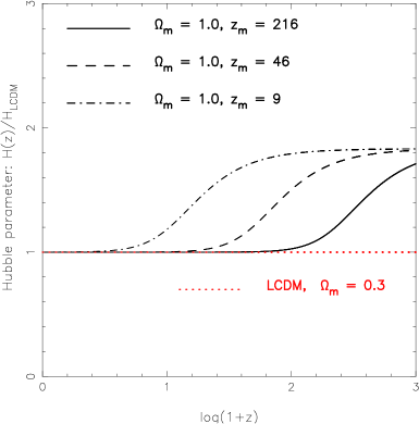
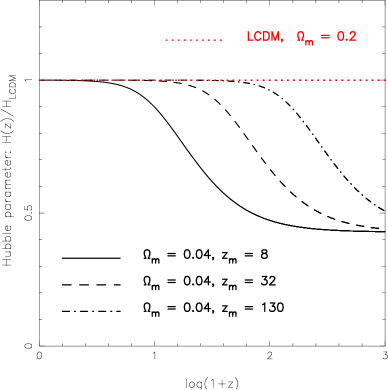
Figure 6: This figure illustrates that $H_{\rm brane}\simeq H_{\rm LCDM}$ for low redshifts, whereas at higher redshifts $H_{\rm brane}>H_{\rm LCDM}$ (for Mimicry 1, shown in the left panel) or $H_{\rm brane}<H_{\rm LCDM}$ (for Mimicry 2, shown in the right panel). This behaviour arises when $\Omega_{\rm m}>\Omega_{\rm m}^{\rm LCDM}$ (Mimicry 1) or $\Omega_{\rm m}<\Omega_{\rm m}^{\rm LCDM}$ (Mimicry 2). See [11] for details of mimicry models and for some cosmological consequences of mimicry.

We remind the reader that the two signs in (56) or (64) correspond to two complementary possibilities for embedding the brane in the higher-dimensional (Schwarzschild-AdS) bulk. In our ensuing discussion, we shall refer to the model with the lower (upper) sign in (64) as Mimicry 1 (Mimicry 2), and we consider these two models separately.

5.2 Cosmological perturbations in the mimicry model:
I. Scale-dependent boundary conditions

As expected, perturbations in the mimicry model crucially depend upon the type of boundary condition which has been imposed. Generally speaking, brane perturbations grow moderately for BC’s which lie in the stability domain (41) or (42) and more rapidly in the instability region. This remains true for mimicry models. In this section, we explore the behaviour of perturbations in this model for the boundary condition $A=0$, which belongs to the instability class. In the next section, we shall explore BC’s which give rise to more moderate and scale-independent behavior.

The growth of perturbations if $A=0$ is substituted in (38) is illustrated in figure 7. The $k$-dependence, clearly seen in this figure, can be understood by inspecting the system of equations (34)–(36). Even if we start with zero initial conditions for the dark-radiation components $\delta\rho_{\cal C}$ and $v_{\cal C}$, the nontrivial right-hand side of Eq. (35) leads to the generation of $v_{\cal C}$; then, via the $k$-dependent right-hand side of (36), the density $\delta\rho_{\cal C}$ is generated, which later influences the growth of perturbations of matter in (34). The instability in the growth of perturbations is explained by the fact that the value of $A=0$ lies outside the stability domain (41) or (42). However, the growth of perturbations is not as dramatic in this case as in the DGP model with the Koyama–Maartens BC’s, mainly because the value $A=0$ lies much closer to the boundary (42) than the Koyama–Maartens value $A=-1/2$.

     

Figure 7: Growth of matter perturbations in the Mimicry 1 and Mimicry 2 models are shown for different values of the comoving wave number $k/a_{0}H_{0}$ (indicated by numbers above the corresponding curves) and for the minimal boundary condition $A=0$ in (38). Both models have the same effective parameter $\Omega^{\rm LCDM}_{\rm m}=0.22$, hence, quite different matter content, indicated by the parameter $\Omega_{\rm m}$. The value of $v_{\cal C}$ is set to zero initially. The position of the mimicry redshift $z_{\rm m}$ is indicated by the vertical dotted lines.

Qualitatively, the evolution of matter perturbations in mimicry models can be understood as follows: during the early stages of matter-domination the last term on the right-hand side of equation (34) is not very important, which transforms (34) into a closed equation for the matter perturbation. Indeed, in the pre-mimicry regime, for $z\gg z_{\rm m}\,$, we have $\left|\ell^{2}\lambda\right|\gg 1$ for the quantity in the denominator of the last term on the right-hand side of (34), which makes this term relatively small for moderate values of $\delta\rho_{\cal C}$. Thus, perturbations in matter evolve according to (46) on all spatial scales, for redshifts greater than the mimicry redshift $z_{\rm m}$. For $z\leq z_{\rm m}$, the quantity $\left|\ell^{2}\lambda\right|$ is of order unity. By this time, the perturbations $\delta\rho_{\cal C}$ have grown large, and their amplitude strongly depends on the wave number. Through the last term in equation (34), they begin to influence the growth of matter perturbations for $z\sim z_{\rm m}$, resulting in the $k$-dependent growth of the latter. The reason for the opposite $k$-dependence of matter perturbations in Mimicry 1 and Mimicry 2 shown in figure 7 is connected with the difference in the sign of $\lambda$ — defined in (32) — for the two models. Thus, the last term in (34) comes with opposite signs in Mimicry 1 and Mimicry 2, and therefore works in opposite directions in these two models.

Well inside the mimicry regime, for $z\ll z_{\rm m}$, we have $\gamma\approx 1/3$, so that the second term on the right-hand side of (35) can be ignored if matter perturbations are not too large. Then equations (35), (36), and (38) lead to a closed system of equations for the evolution of dark-radiation perturbations. Substituting $\gamma=1/3$ into this system, we obtain:

$$v_{\cal C}=a^{-7/2}\xi\,,\qquad\delta\rho_{\cal C}={3\over(1+2A)a^{3}}{\partial\over\partial t}\left(a^{3}v_{\cal C}\right)\,,$$ (69)

where we assumed $A\not\approx-1/2$ to be constant. The function $\xi$ obeys an oscillator-type equation

$$\ddot{\xi}-\left(\frac{1}{2}\dot{H}+\frac{1}{4}H^{2}+{1+2A\over 3a^{2}}\nabla^{2}\right)\xi=0\,.$$ (70)

This means that both $\delta\rho_{\cal C}$ and $v_{\cal C}$ rapidly decay during the mimicry regime (oscillating approximately in opposite phase) and the last term on the right-hand side of (34) again becomes unimportant. In particular, this will describe the behaviour of the mimicry model with the minimal boundary condition $A=0$. The transient oscillatory character of $\delta\rho_{\cal C}$ induces transient oscillations with small amplitude in $\Delta$ through the last term in (36). These small oscillations can be noticed in figure 7 for $\log\,(1+z)\ \lower-2.0pt\vbox{\hbox{\hbox to0.0pt{$>$\hss}\lower 5.5pt\vbox{\hbox{$\sim$}}}}\ 1$, particularly for values $40$ and $30$ of the comoving wave number.

Two important features of mimicry models deserve to be highlighted:

1. As demonstrated in figure 7, there is a strong suppression of long-wavelength modes in Mimicry 2.

2. From this figure, we also find that the growth of short-wavelength modes in Mimicry 2 can be substantial, even in a low-density universe.

Both properties could lead to interesting cosmological consequences. For instance, the relative suppression of low-$k$ modes may lead to a corresponding suppression of low-multipole fluctuations in the cosmic microwave background, while the increased amplitude of high-$k$ modes could lead to an earlier epoch of structure formation. (Since the mimicry models behave as LCDM at low redshifts, they satisfy the supernova constraints quite well.) A detailed investigation of both effects, however, requires that we know the form of the transfer function of fluctuations in matter (and dark radiation) at the end of the radiative epoch. Such an investigation lies outside the scope of the present paper, but we may return to it elsewhere.

For the minimal boundary condition ($A=0$), assumed in this section, equations (28) and (39) imply $\Phi=\Psi$ and

$${1\over a^{2}}\nabla^{2}\Phi=\left(1+{2\over\ell^{2}\lambda}\right){\Delta_{\rm m}\over 2m^{2}}+{\Delta_{\cal C}\over m^{2}\ell^{2}\lambda}\,,$$ (71)

which is a generalization of the Poisson equation for the mimicry brane.

Mimicry models with the Koyama–Maartens boundary condition exhibit much stronger instability in the growth of $\delta\rho_{\cal C}$ for high values of $k$, enhancing the growth of matter perturbations (not shown). This can be explained by the fact that $A=0$ is much closer to the boundary of the stability domain (42) than the Koyama–Maartens value $A=-1/2$. For the latter, the density perturbation $\Delta$ in the Mimicry 1 model grows to be large and negative, while the perturbation $\delta\rho_{\cal C}$ becomes large and positive; for instance, both $\Delta$ and the dimensionless quantity $\delta\rho_{\cal C}/m^{2}H^{2}$ grow by a factor of $10^{11}$ for $k/a_{0}H_{0}=40$. This provides another example of the very strong dependence of perturbation evolution on boundary conditions.

In our calculations, we have not found any significant dependence of the eventual growth of perturbations on initial conditions for dark radiation specified in a reasonable range (at $z=10^{3}$).

5.3 Cosmological perturbations in the Mimicry model:
II. Scale-free boundary conditions

As mentioned earlier, BC’s lying in the stability region (41) lead to an almost scale-free growth of density perturbations. A similar result is obtained if we assume the scale-free boundary condition (45) of section 3.2. In this case, the momentum potential $v_{\cal C}$ decays as $v_{\cal C}\propto a^{-4}$, and its spatial gradients in (36) can therefore be neglected. The same is true, of course, if one considers super-horizon modes with $k\ll aH$. In both cases, we have approximately $\delta\rho_{\cal C}\propto 1/a^{4}$, suggesting that the dynamical role of perturbations in dark radiation is unimportant. This results in a radical simplification: as in the DGP model, for BC’s lying in the stability region, the growth of perturbations in matter can be effectively described by a single second-order differential equation (46), namely,

$$\ddot{\Delta}+2H\dot{\Delta}=\Theta\,{\rho\Delta\over 2m^{2}}\,,\qquad\Theta=\left(1+{6\gamma\over\ell^{2}\lambda}\right)\,,$$ (72)

where $\lambda$ and $\gamma$ are defined in (31) and (32), respectively. We shall call $\Theta(z)$ in (72) the ‘gravity term’ since it incorporates the effects of modified gravity on the growth of perturbations. The value of this term on the brane can depart from the canonical $\Theta=1$ in general relativity.

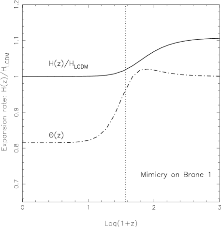
Figure 8: The Hubble parameter in the braneworld ‘Mimicry 1’ is shown relative to LCDM (solid). The LCDM model has $\Omega^{\rm LCDM}_{\rm m}=0.22$ while $\Omega_{\rm m}=0.27$ on the brane. Also shown is the ‘gravity term’ $\Theta(z)$ defined in (46) whose value diminishes from unity at high redshifts to the asymptotic form (73) at low redshifts. The dotted vertical line shows the mimicry redshift $z_{m}\approx 37$.

Figure 8 shows the behaviour of $\Theta(z)$ for a typical mimicry model. At redshifts significantly larger than the mimicry redshift, $z\gg z_{\rm m}$, we have $\Theta(z)\simeq 1$, whereas at low redshifts, $z\ll z_{\rm m}$, the value of $\Theta(z)$ changes to

$$\Theta(z)\simeq\frac{\Omega^{\rm LCDM}_{\rm m}}{\Omega_{\rm m}}=\frac{\rho^{\rm LCDM}}{{\rho}}\quad\mbox{for}\quad z\ll z_{\rm m}\,,$$ (73)

where $\rho^{\rm LCDM}$ is defined in (62). The solid line in the same figure shows the ratio of the Hubble parameter on the brane to that in LCDM. The consequences of this behaviour for the growth equation (46) are very interesting. Substituting (73) into (46) and noting that $H(z)\simeq H^{\rm LCDM}$ during mimicry, we recover the standard equation describing perturbation growth in the LCDM model

$${\ddot{\Delta}}+2H^{\rm LCDM}\dot{\Delta}={\rho^{\rm LCDM}\Delta\over 2m^{2}}\,.$$ (74)

Thus, ordinary matter in mimicry models gravitates in agreement with the effective value of the gravitational constant which appears in the cosmological equations (58) and (60).

Figure 9: Density perturbations on the Mimicry 1 brane (dot-dash) and in LCDM (solid). The evolution of perturbations in Mimicry 1 in this case is effectively described by (46). In both cases, the perturbation amplitude is scaled by the expansion factor $a(t)$. (It may be noted that $\Delta/a=1$ in standard CDM with $\Omega_{\rm m}=1$.) The dotted vertical line shows the mimicry redshift $z_{\rm m}\approx 37$. The braneworld has $\Omega_{\rm m}=0.27$ while $\Omega^{\rm LCDM}_{\rm m}=0.22$. This leads to a moderate enhancement in the amplitude of brane perturbations over LCDM.

We therefore conclude that, deep in the mimicry regime ($z\ll z_{\rm m}$), perturbations grow at the same rate on the brane and in LCDM. This is borne out by figure 9, which shows the results of a numerical integration of (46) for Mimicry 1 [integrating the exact system (34)–(36) gives indistinguishable results]. Notice that the total amplitude of fluctuations during mimicry in this model is greater on the brane than in LCDM. Indeed, for mimicry models, we have

$$\frac{\Delta_{\rm brane}}{\Delta_{\rm LCDM}}\simeq\frac{\Omega_{\rm m}}{\Omega^{\rm LCDM}_{\rm m}}\quad\mbox{for}\quad z\ll z_{\rm m}\,,$$ (75)

and this ratio is greater than unity for Mimicry 1.

Since the contribution from perturbations in dark radiation can be neglected, the growth of matter perturbations in Mimicry 2 is again described by (46) and by (75). However, since $\Omega_{\rm m}<\Omega^{\rm LCDM}_{\rm m}$ in this case, the final amplitude of perturbations will be smaller in Mimicry 2 than the corresponding quantity in LCDM, which is the opposite of what we have for Mimicry 1.

It is interesting that during mimicry, when $\gamma\approx 1/3$, the relation between the gravitational potentials $\Phi$ and $\Psi$ reduces to the general-relativistic form $\Phi=\Psi$, as can be seen from (48), where $\Phi$ satisfies the generalized Poisson equation (47), namely,

$${1\over a^{2}}\nabla^{2}\Phi=\Theta{\Delta_{\rm m}\over 2m^{2}}\,.$$ (76)

An interesting feature of Mimicry 1 is that, at early times, the expansion rate in this model exceeds that in LCDM, i.e., $H(z)|_{\rm Mimicry1}>H(z)|_{\rm LCDM}$ for $z>z_{\rm m}$ (see Figs. 6 & 8). [The opposite is the case for Mimicry 2: the expansion rate in this model is lower than that in LCDM at early times, i.e., $H(z)|_{\rm Mimicry\,2}<H(z)|_{\rm LCDM}$ for $z>z_{\rm m}$.] As we can see, this has important consequences for the growth of structure in this model. The increase in the growth of perturbations in Mimicry 1 relative to LCDM occurs during the period before and slightly after the mimicry redshift has been reached, when the relative expansion rate $H(z)/H^{\rm LCDM}$ is declining while the ‘gravity term’ $\Theta(z)$ has still not reached its asymptotic form (73). A lower value of $H(z)$ in (46) diminishes the damping of perturbations due to cosmological expansion while a slower drop in $\Theta(z)$ signifies a much more gradual decrease in the force of gravity. Consequently, there is a net increase in the growth of perturbations on the Mimicry 1 brane relative to LCDM. For the models in figure 9, which have $\Omega^{\rm LCDM}_{\rm m}=0.22$ and $\Omega_{\rm m}=0.27$, the increase is about $20\%$. The increased amplitude of perturbations in Mimicry 1 stands in contrast to the DGP model as well as Quintessence model, in both of which linearized perturbations grow at a slower rate than in the LCDM cosmology [6, 7, 29].

It is important to note that observations of galaxy clustering by the 2dFGRS survey provide the following estimate [30] for perturbation growth at a redshift $z=0.15$ :

$${d\log\delta\over d\log a}\equiv-\left.(1+z)\frac{d\log\delta}{dz}\right|_{z=0.15}=0.51\pm 0.11\,,$$ (77)

where $\delta\equiv\delta\rho/\rho$. Since the growth of perturbations during the mimicry regime stays proportional to that in the LCDM model ($\delta_{\rm mimic}\propto\delta_{\rm LCDM}$, $z\ll z_{\rm m}$), it follows that if perturbations in the LCDM model satisfy (77) (which they do), then so will those in the mimicry scenario. Nevertheless, as we have seen, the net increase in the amplitude of perturbations on the brane is larger than that in the LCDM model. This clearly has important cosmological consequences since it can enhance structure formation at high redshifts as well as lead to higher values of $\sigma_{8}$. Thus, while preserving the many virtues of the LCDM model, the mimicry models add important new features which could be tested by current and future observations. We hope to return to some of these issues in a future work.

6 Discussion

Braneworld theories with large extra dimensions, while having a number of very attractive properties, also have a common difficulty: on the one hand, the dynamics of the higher-dimensional bulk space needs to be taken into account in order to understand brane dynamics; on the other hand, all observables are restricted to the four-dimensional brane. In field-theoretic language, the situation can be described in terms of an infinite (quasi)-continuum of Kaluza–Klein gravitational modes existing on the brane from the brane viewpoint. This property makes braneworld theory complicated, solutions on the brane non-unique and evolution nonlocal. For instance, while the solution with a spherically symmetric source is relatively simple and straightforward in general relativity, a similar problem in braneworld theory does not appear to have a unique solution (see, e.g., [31]).

Fortunately, in situations possessing a high degree of symmetry, the above properties of braneworld theory do not affect its cosmological solutions (at least, in the simplest case of one extra dimension). Thus, homogeneous and isotropic cosmology on the brane is almost uniquely specified since it involves only one additional integration constant which is associated with the mass of a black hole in the five-dimensional bulk space. This makes braneworld theory an interesting alternative for modelling dark-energy [22] and dark-matter [11] effects on cosmological scales.

However, in order to turn a braneworld model into a complete theory of gravity viable in all physical circumstances, it is necessary to address the issue of boundary conditions. Usually, one tries to formulate reasonable conditions in the bulk by demanding that the bulk metric be nonsingular or by employing other (regulatory) branes. However, neither of these conditions have been implemented in braneworld theory in full generality; moreover, they leave open the problem of nonlocality of the gravitational laws on the brane (since the brane is left open to influences from the bulk).

In this paper, we adopted a different approach to the issue of boundary conditions in the brane–bulk system. From a broader perspective, boundary conditions can be regarded as any conditions restricting the space of solutions. Our approach is to specify such conditions directly on the brane which represents the observable world, in order to arrive at a local and closed system of equations on the brane. The behaviour of the metric in the bulk is of no further concern in this approach, since this metric is for all practical purposes unobservable. Since the nonlocality of the braneworld equations is known to be connected with the dynamical properties of the bulk Weyl tensor projected onto the brane [15], it is natural to consider the possibility of imposing certain restrictions on this tensor. Perhaps, the simplest condition is to set to zero its (appropriately defined) anisotropic stress. This is fully compatible with all the equations of the theory and results in a brane universe described by a modified theory of gravity and having an additional invisible component — dark radiation — which is endowed with nontrivial dynamics. More generally, we suggest (17) and (38) which describes a one-parameter family of BC’s with the parameter $A$. This family generalizes the boundary condition derived by Koyama and Maartens [7] for the DGP model in the small-scale and quasi-static approximation (Koyama and Maartens derived the value $A=-1/2$).

An important conclusion of our paper is that the growth of perturbations in braneworld models strongly depends upon our choice of BC’s. This was illustrated in figure 5 for the DGP model. Specifying boundary conditions in the form (38) allows us to determine regions of stability and instability in terms of the single parameter $A$; they are described by Eq. (41). In the DGP model, perturbations are explicitly demonstrated to be quasi-stable for $A=1/2$ (figure 4) and unstable for $A=-1/2$ (figure 2). In the instability domain, gradients in the momentum potential $v_{\cal C}$ of dark radiation, lead to the creation of perturbations in this quantity via equation (35). This effect can significantly boost the growth of perturbations in matter. An important implication of this effect is that perturbations in the baryonic component might overcome the ‘growth problem,’ which plagues them in standard general relativity, and grow to acceptable values without requiring the presence of (deep potential wells in) dark matter. The Mimicry 2 model looks promising from this perspective. Note that, in this model, the expansion of a low-density universe is virtually indistinguishable from that of a (higher-density) LCDM model. Enhanced perturbation growth in this ‘mimicry’ model might permit a low-density universe to also match observations of gravitational clustering (thereby circumventing the need for large amounts of dark matter to achieve this purpose). A detailed investigation of this effect, however, lies outside the scope of the present paper and will be taken up elsewhere.

Values of $A$ lying in the stability region (41) or a scale-free boundary condition such as (45) may also be important. In this case, perturbations in the DGP model grow slower than in LCDM whereas perturbations in Mimicry 1 grow somewhat faster. This suggests that structure formation may occur slightly earlier in Mimicry 1 than it does in LCDM.

Two related points deserve mention. In general relativity, the linearized perturbation equation

$${\ddot{\delta}}+2H{\dot{\delta}}=\frac{3}{2}H_{0}^{2}\Omega_{\rm m}\left(\frac{a_{0}}{a}\right)^{3}\delta$$ (78)

depends exclusively upon the expansion history of the universe and the value of $\Omega_{\rm m}$, so that a knowledge of $H(z)$ from independent sources (such as the luminosity distance) permits one to determine $\delta(z)$ and, vice-versa, the observed value of $\delta(z)$ can be used to reconstruct the expansion history $H(z)$ [34]. As we have demonstrated in this paper, equation (78) is no longer valid for the braneworld, and it remains to be seen whether knowing $H(z)$ and $\Omega_{\rm m}$ will allow us to reconstruct $\delta(z)$ uniquely.

It is also well known that the expansion history, $H(z)$, does not characterize a given world model uniquely, and it is conceivable that cosmological models having fundamentally different theoretical underpinnings (such as different forms of the matter Lagrangian or different field equations for gravity) could have identical expansion histories (some examples may be found in [34] which also contains references to earlier work). As an illustration, consider the Brane 2 model in which the effective equation of state is never phantom-like, so that $w_{\rm eff}\geq-1$. As we have seen, Mimicry 2 and the DGP model form important subclasses of this braneworld. A quintessence potential corresponding to a given expansion history can be determined from [35]

$${8\pi G\over 3H_{0}^{2}}V(x)\ = {H^{2}\over H_{0}^{2}}-{x\over 6H_{0}^{2}}{dH^{2}\over dx}-\frac{1}{2}\Omega_{\rm m}\,x^{3}\,,$$ (79)

$${8\pi G\over 3H_{0}^{2}}\left({d\phi\over dx}\right)^{2} = {2\over 3H_{0}^{2}x}{d\ln H\over dx}-{\Omega_{\rm m}x\over H^{2}}\,,\quad x\equiv 1+z\,.$$ (80)

Substitution for $H(z)$ from (18) with the plus sign results in a quintessence model which has the same expansion history as the braneworld. Perturbative effects, however, are likely to break this degeneracy, since it is unlikely that matter perturbations will grow at the same rate in the quintessence model as on the brane.

Although we have explicitly solved the perturbation equations only for two cases: the mimicry models [11] and the DGP braneworld [2], it is quite clear that the treatment developed by us may have larger ramifications since it could be applied to a broader class of models. In [36], for instance, it was shown that a braneworld dual to the Randall–Sundrum II model — the bulk dimension being time-like instead of space-like — will bounce at early times, thereby avoiding the singularity problem which plagues general relativity. It would be an interesting exercise to apply the formalism developed in this paper to this non-singular braneworld to see if the problem of tachyonic gravitational modes can be avoided. Since the boundary conditions of type (10)–(17), specified directly on the brane, effectively freeze certain degrees of freedom in the brane–bulk system, the corresponding braneworld theory may also be free from the debatable problem of ghosts (see [37] for a recent discussion of this problem).

Whether boundary conditions such as those described by equations (10)–(17) or (45) will remain in place for a more fundamental extra-dimensional theory is presently a moot point. Perhaps, by comparing the consequences of different boundary conditions with observations we will gain a better understanding of the type of braneworld theory most consistent with reality.

We believe that our calculations have opened up an interesting avenue for further research in braneworld cosmology. Related astrophysical phenomena which demand further exploration include gravitational lensing, fluctuations in the cosmic microwave background, the power spectrum of density fluctuations, etc. For a deeper understanding of gravitational instability on the brane, we also need to examine the behaviour of perturbations during the radiative epoch as well as their origin as vacuum fluctuations (presumably) during inflation. Additional issues of considerable interest relate to non-linear gravitational clustering on the brane. For instance, it is well known that a density field which was originally Gaussian develops non-Gaussian features even in the weakly non-linear regime of gravitational instability [38]. Although these effects do not appear to be unduly sensitive to the presence of dark energy, this has only been tested for $\Lambda$CDM and a few other conventional dark-energy models [39]. The value of the lower moments of the density field such as its skewness $\langle\delta^{3}\rangle/\langle\delta^{2}\rangle^{2}$ and kurtosis $\langle\delta^{4}\rangle/\langle\delta^{2}\rangle^{3}$ in models which give rise to acceleration because of amendments to the gravitational sector of the theory remain unexplored and could lead to a deeper understanding of structure formation in these models.

We hope to return to some of these issues in the future.

Appendix A Attempts at deriving boundary conditions

Recent attempts at deriving proper boundary conditions for the brane–bulk system by considering perturbations in the bulk were made in [7, 8]. Here we would like to discuss this approach in more detail and illustrate some difficulties with this treatment.

Both approaches study perturbation in the DGP model, which has Minkowski bulk background, and use the Mukohyama master equation [9] for the scalar variable $\Omega(t,{\vec{x}},y)$ written in Gaussian normal coordinates with respect to the brane, which is located at $y=0$ in the fifth coordinate $y$ and has intrinsic coordinates $\{t,{\vec{x}}\}$:

$$-{\partial\over\partial t}\left({1\over nb^{3}}{\partial\Omega\over\partial t}\right)+{\partial\over\partial y}\left({n\over b^{3}}{\partial\Omega\over\partial y}\right)-{nk^{2}\over b^{5}}\Omega=0\,,$$ (81)

where

$$n(t,y)=1+\left({\dot{H}\over H}+H\right)y\,,\qquad b(t,y)=a\left(1+Hy\right)$$ (82)

are the functions describing the unperturbed bulk metric

$$ds^{2}=-n^{2}dt^{2}+b^{2}d{\vec{x}}^{2}+dy^{2}\,,$$ (83)

and $k$ is the wave number in the Fourier decomposition in the ${\vec{x}}$ space.

The (suitably normalized) Mukohyama variable is related to perturbations on the DGP brane via [10]:

$$\begin{array}[]{l}\displaystyle\delta\rho_{\cal C}=-{k^{4}\over 3a^{5}}\left.\Omega\right|_{y=0}\,,\vskip 6.0pt plus 2.0pt minus 2.0pt\\ \displaystyle v_{\cal C}={k^{2}\over 3a^{3}}\left.\left(\dot{\Omega}-H\Omega\right)\right|_{y=0}\,,\vskip 6.0pt plus 2.0pt minus 2.0pt\\ \displaystyle\delta\pi_{\cal C}=-{1\over 6a}\left.\left(3\ddot{\Omega}-3H\dot{\Omega}+{k^{2}\over a^{2}}\Omega+3\dot{H}\left(\ell-H^{-1}\right){\partial\Omega\over\partial y}\right)\right|_{y=0}\,.\end{array}$$ (84)

Koyama and Maartens [7] study perturbations on subhorizon scales, $k\gg aH$, and employ what they call ‘quasi-static approximation,’ which consists in neglecting the time derivatives in (81) and (84). By considering the approximate ‘quasi-static’ solution for $\Omega$ with appropriate (decaying) boundary condition in the bulk, they argue that the term with the derivative $\partial\Omega/\partial y$ in the brackets on the right-hand side of the last relation in (84) can also be neglected, and this relation then becomes

$$\delta\pi_{\cal C}\approx-{k^{2}\over 6a^{3}}\left.\Omega\right|_{y=0}\,.$$ (85)

This results in the Koyama–Maartens boundary condition (38), (43).

However, as was shown in the paper, the boundary condition (38), (43) leads directly to equation (3.2), which exhibits strong scale-dependent instability. The last effect was also demonstrated numerically. We note that, in deriving equation (3.2), we used the exact system of equations (34)–(36) on the brane, and we did not perform any time differentiation of the approximate relation (38), which might be illegitimate in the quasi-static approximation. This means, in our view, that the quasi-static approximation, which was assumed in deriving conditions (85), cannot hold during the whole course of evolution described by the system of equations for perturbations (34)–(36).

Sawicki, Song, and Hu [8] study scalar perturbations on all scales. They note that the distance $y_{\rm hor}$ to the causal horizon of the brane remains proportional to $H^{-1}$ during periods of domination of matter with constant equation of state, and they impose the zero boundary condition for $\Omega$ at this causal horizon. This does not fix the value of $\Omega$ at the brane, and it is done separately by setting a ‘scaling’ ansatz of the form

$$\Omega=A(p)a^{p}G\left(x,{k\over aH}\right)\,,\qquad x={y\over y_{\rm hor}}\,,\qquad y_{\rm hor}=\xi H^{-1}\,.$$ (86)

They substitute (86) into (81) to derive a differential equation on $G\left(x,{k\over aH}\right)$ during periods of domination of a fluid with constant equation of state (radiation or matter). In doing this, they treat $p$, $A(p)$, and $\xi$ as constants and also neglect the derivative of $G\left(x,{k\over aH}\right)$ with respect to the second argument. One cane note that this already imposes certain restriction on the form of $\Omega$ on the brane, hence, via (84), also on the perturbations of dark radiation. The result is the differential equation for $G\left(x,{k\over aH}\right)$ of the form

$${\partial^{2}G\over\partial x^{2}}+f_{1}(p,x){\partial G\over\partial x}+\left[f_{0}(p,x)-\left({k\over aH}\right)^{2}g(p,x)\right]G=0\,,$$ (87)

where $f_{0}$, $f_{1}$, and $g$ are some functions, and in which the quantity ${k\over aH}$ plays the role of a parameter. This equation is solved with the boundary conditions $G(0)=1$, $G(1)=0$, which uniquely determines the derivative $G^{\prime}(0)$, hence, the quantity $\partial\Omega/\partial y$ on the brane needed in (84).

The power $p$ in (86) is not yet specified, and it is adjusted in [8] by an iterative procedure so as to satisfy the Bianchi identity on the brane coupled to the cosmological equations for matter perturbations. In this way, $p$ also becomes a function of the scale factor $a$.

One can see that a number of assumptions were made in this procedure. In deriving equation (87), the time derivatives of $p$ and the partial derivative of $G\left(x,{k\over aH}\right)$ with respect to its second argument were neglected. Together with ansatz (86), this means that an effective ‘quasi-static’ approximation was used for $\Omega$, similar to the one employed in [7]. It is not surprising, therefore, that, on subhorizon scales, the result of [7] is reproduced, with the approximate relations (38), (43), for which the quasi-static regime is unstable, as we have shown in this paper.

Furthermore, the authors did not extend smoothly their approximate solution in the bulk beyond the horizon $y=y_{\rm hor}$, so it is not at all clear whether it is really singularity-free in the bulk, as was claimed. To specify simply $\Omega\equiv 0$ for $y\geq y_{\rm hor}$ means introducing a discontinuity in the derivative of $\Omega$ at $y=y_{\rm hor}$, which itself can be regarded as a singularity. This once again illustrates the general difficulty which one encounters in finding singularity-free solutions in the bulk.

References

References

-
[1]
Randall L and Sundrum R 1999 Phys. Rev. Lett. 83 3370 (Preprint arXiv:hep-ph/9905221)
Randall L and Sundrum R 1999 Phys. Rev. Lett. 83 4690 (Prepront arXiv:hep-th/9906064) -
[2]
Dvali G, Gabadadze G and Porrati M 2000 Phys. Lett. B 485 208
(Preprint arXiv:hep-th/0005016)
Dvali G and Gabadadze G 2001 Phys. Rev. D 63 065007 (Preprint arXiv:hep-th/0008054) -
[3]
Binetruy P, Deffayet C and Langlois D 2000 Nucl. Phys. B 565 26
(Preprint arXiv:hep-th/9905012)
Binetruy P, Deffayet C, Ellwanger U and Langlois D 2000 Phys. Lett. B 477 285 (Preprint arXiv:hep-th/9910219) -
[4]
Collins H and Holdom B 2000 Phys. Rev. D 62 105009 (Preprint arXiv:hep-ph/0003173)
Shtanov Yu V 2000 On brane-world cosmology Preprint arXiv:hep-th/0005193 -
[5]
Deffayet C 2001 Phys. Lett. B 502 199 (Preprint arXiv:hep-th/0010186)
Deffayet C, Dvali G and Gabadadze G 2002 Phys. Rev. D 65 044023 (Preprint arXiv:astro-ph/0105068) -
[6]
Lue A, Scoccimarro R and Starkman G D 2004 Phys. Rev. D 69 124015
(Preprint arXiv:astro-ph/0401515)
Lue A 2006 Phys. Rept. 423 1 (Preprint arXiv:astro-ph/0510068) -
[7]
Koyama K and Maartens R 2006 JCAP 0601 016 (2006)
(Preprint arXiv:astro-ph/0511634)
Koyama K 2006 JCAP 0603 017 (Preprint arXiv:astro-ph/0601220) - [8] Sawicki I, Song Y-S and Hu W 2007 Phys. Rev. D 75 064002 (Preprint arXiv:astro-ph/0606285)
- [9] Mukohyama S 2000 Phys. rev. D 62 084015 (Preprint arXiv:hep-th/0004067)
-
[10]
Deffayet C 2002 Phys. Rev. D 66 103504 (Preprint
arXiv:hep-th/0205084)
Deffayet C, 2005 Phys. Rev. D 71 023520 (Preprint arXiv:hep-th/0409302) - [11] Sahni V, Shtanov Yu and Viznyuk A 2005 JCAP 0512 005 (Preprint arXiv:astro-ph/0505004)
- [12] Maartens R 2003 Prog. Theor. Phys. Suppl. 148 213 (Preprint arXiv:gr-qc/0304089)
- [13] Barrow J D and Maartens R 2002 Phys. Lett. B 532 153 (Preprint arXiv:gr-qc/0108073)
-
[14]
Kofinas G, Papantonopoulos E and Zamarias V 2002 Phys. Rev. D 66
104028 (Preprint arXiv:hep-th/0208207)
Harko T and Mak M K 2004 Phys. Rev. D 69 064020 (Preprint arXiv:gr-qc/0401049) - [15] Shiromizu T, Maeda K and Sasaki M 2000 Phys. Rev. D 62 024012 (Preprint arXiv:gr-qc/9910076)
-
[16]
Song Y-S 2005 Phys. Rev. D 71 024026 (Preprint
arXiv:astro-ph/0407489)
Knox L, Song Y-S and Tyson J A 2005 Two Windows on Acceleration and Gravitation: Dark Energy or New Gravity? Preprint arXiv:astro-ph/0503644
Sawicki I and Carroll S M 2005 Cosmological Structure Evolution and CMB Anisotropies in DGP Braneworlds Preprint arXiv:astro-ph/0510364 -
[17]
Mak M K and Harko T 2004 Phys. Rev. D 70 024010
(Preprint arXiv:gr-qc/0404104)
Harko T and Cheng K S 2006 Astrophys. J. 636 8 (Preprint arXiv:astro-ph/0509576) -
[18]
Pal S, Bharadwaj S and Kar S 2005 Phys. Lett. B 609 194
(Preprint arXiv:gr-qc/0409023)
Pal S 2005 Phys. Teacher 47 144 (Preprint arXiv:astro-ph/0512494) - [19] Viznyuk A and Shtanov Yu 2007 Phys. Rev. D 76 064009 (Preprint arXiv:0706.0649)
- [20] Wald R M 1984 General Relativity (Chicago: The University of Chicago Press)
- [21] Sakharov A D 1967 Dokl. Akad. Nauk SSSR. Ser. Fiz. 177 70 [1968 Sov. Phys. Dokl. 12 1040] reprinted in: 1991 Usp. Fiz. Nauk 161 64 [1991 Sov. Phys. Usp. 34 394]; 2000 Gen. Rel. Grav. 32 365
- [22] Sahni V and Shtanov Yu 2003 JCAP 0311 014 (Preprint arXiv:astro-ph/0202346)
- [23] Sahni V and Shtanov Yu 2005 Phys. Rev. D 71 084018 (Preprint arXiv:astro-ph/0410221)
- [24] Sahni V Cosmological Surprises from Braneworld models of Dark Energy, Proceedings of the 14th Workshop on General Relativity and Gravitation (JGRG14), Kyoto University, Japan, 29 November – 3 December, 2004. Edited by W. Hikida, M. Sasaki, T. Tanaka and T. Nakamura, pp.95–115 (Preprint arXiv:astro-ph/0502032)
-
[25]
Alam U and Sahni V 2006 Phys. Rev. D 73 084024 (Preprint
arXiv:astro-ph/0511473)
Maartens R and Majerotto E 2006 Phys. Rev. D 74 023004 (Preprint arXiv:astro-ph/0603353)
Szydłowski M and Godłowski W 2006 Phys. Lett. B 639 5 (Preprint arXiv:astro-ph/0511259) -
[26]
Maartens R 2000 Phys. Rev. D 62 084023 (Preprint
arXiv:hep-th/0004166)
Langlois D 2000 Phys. Rev. D 62 126012 (Preprint arXiv:hep-th/0005025)
Langlois D 2001 Phys. Rev. Lett. 86 2212 (Preprint arXiv:hep-th/0010063)
Langlois D, Maartens R, Sasaki M and Wands D 2001 Phys. Rev. D 63 084009 (Preprint arXiv:hep-th/0012044)
Bridgman H A, Malik K A and Wands D 2002 Phys. Rev. D 65 043502 (Preprint arXiv:astro-ph/0107245) -
[27]
Mukohyama S 2000 Phys. Lett. B 473 241 (Preprint
arXiv:hep-th/9911165)
Koyama K and Soda J 2002 Phys. Rev. D 65 023514 (Preprint arXiv:hep-th/0108003) - [28] Ishak M, Upadhye A and Spergel D N 2006 Phys. Rev. D 74 043513 (Preprint arXiv:astro-ph/0507184)
-
[29]
Wang L and Steinhardt P 1998 Astrophys. J. 508 483 (Preprint arXiv:astro-ph/9804015)
Benabed K and Bernardeau F 2001 Phys. Rev. D 64 083501 (Preprint arXiv:astro-ph/0104371) -
[30]
Verde L et al 2002 MNRAS 335 432 (Preprint
arXiv:astro-ph/0112161)
Hawkins E et al 2003 MNRAS 346 78 (Preprint arXiv:astro-ph/0212375) - [31] Majumdar A S and Mukherjee N 2005 Int. J. Mod. Phys. D 14 1095 (Preprint arXiv:astro-ph/0503473)
- [32] Clowe D et al 2006 A direct empirical proof of the existence of dark matter Preprint arXiv:astro-ph/0608407
-
[33]
Sahni V, Feldman H and Stebbins A 1992 Astrophys. J. 385 1
Skordis C, Mota D F, Ferreira P G and Boehm C 2006 Phys. Rev. D 96 011301 (Preprint arXiv:astro-ph/0505519)
Skordis C 2006 Phys. Rev. D 74 103513 (Preprint arXiv:astro-ph/0511591)
Dodelson S and Liguori M 2006 Can Cosmic Structure form without Dark Matter? Preprint arXiv:astro-ph/0608602 -
[34]
Sahni V and Starobinsky A A 2000 Int. J. Mod. Phys. D 9 373 (Preprint arXiv:astro-ph/9904398)
Sahni V and Starobinsky A A 2006 Int. J. Mod. Phys. D 15 2105 )Preprint arXiv:astro-ph/0610026) -
[35]
Starobinsky A A 1998 JETP Lett. 68 757 (Preprint
arXiv:astro-ph/9810431)
Saini T D, Raychaudhury S, Sahni V and Starobinsky A A 2000 Phys. Rev. Lett. 85 1162 (Preprint arXiv:astro-ph/9910231) - [36] Shtanov Yu and Sahni V 2003 Phys. Lett. B 557 1 (Preprint arXiv:gr-qc/0208047)
-
[37]
Charmousis C, Gregory R, Kaloper N and Padilla A 2006 JHEP 0610 066
(Preprint arXiv:hep-th/0604086)
Deffayet C, Gabadadze G and Iglesias A 2006 JCAP 0608 012 (Preprint arXiv:hep-th/0607099) -
[38]
Munshi D, Sahni V and Starobinsky A A 1994 Astrophys. J. 436 517
(Preprint arXiv:astro-ph/9402065)
Sahni V and Coles P 1995 Phys. Rept. 262 1 (Preprint arXiv:astro-ph/9505005) -
[39]
Tatekawa T and Mizuno S 2006 JCAP 0602 006 (Preprint
arXiv:astro-ph/0511688)
Tatekawa T and Mizuno S 2006 JCAP 0702 015 (Preprint arXiv:astro-ph/0608691)