Modified gravity with $f(R)=\sqrt{R^{2}-R_{0}^{2}}$

Abstract

Here in this work we propose a modified gravity with the action of $f(R)=\sqrt{R^{2}-R_{0}^{2}}$ instead of Einstein-Hilbert action to describe the late time acceleration of the universe. We obtain the equation of the modified gravity both in the metric and Palatini formalisms. An asymptotic solution of gravity equations corresponding to a constant Ricci scalar causes a late time acceleration of the universe. We do a conformal transformation in the action of the modified gravity and obtain the equivalent minimally coupled scalar-tensor gravity. The equivalent Brans-Dicke gravity of this model is also studied. To examine this model with the observation, the perihelion Precession of the Mercury is compared with our prediction and we put an upper constraint of $R_{0}<H_{0}^{2}$. This range for $R_{0}$ is also in agreement with the cosmological acceleration at the present time. Finally we show that this action has instability for the small perturbations of the metric in vacuum solution in which adding a quadratic term of Ricci scalar can stabilize it.

I Introduction

Recent cosmological data from the Supernova Type Ia (SNIa) and Cosmic Microwave Background (CMB)Ben03 ; Net01 ; Hal02 indicate that universe is currently in the accelerating phase of expansion. The effect of acceleration of the universe on the Supernova Type Ia (SNIa) is making their apparent luminosity dimmer than our expectation R04 ; Perl99 ; Tor03 . The cosmological constant can explain this observational effect. The best fit of the data with the standard (Friedmann Robertson Walker) FRW model results an energy density of $10^{-47}Gev^{4}$ for the cosmological constant. This value is a 55 order of magnitude smaller than the energy density of vacuum in quantum field theory (for review seeCar100 ; Peeb103 ). The cosmological constant is a geometrical term, however it can be regarded as a perfect fluid with the equation of state of $w=-1$. This equation of state provides a constant density during the expansion of the universe. To have the present universe the cosmological constant should be fine-tuned and a small change in this term induces a dramatic change in the destiny of universe.

To solve the cosmological constant problem, the Quintessence model as a time varying cosmological constant due to slow rolling of a scalar field is proposed. This model can cure the fine-tuning problem at the early universe, however there is no physical candidate for the origin of this scalar field peb88 ; wet88 ; sah99 ; arm00 ; pad03 ; cal02 ; cal03 ; w04 ; mov06 ; Arm99 ; Mers01 ; carTr03 ; par99 . The other alternative approach dealing with the acceleration problem of the universe is changing the gravity law through the modification of action of gravity by means of using $f(R)$ instead of the Einstein-Hilbert action. Some of these models as $1/R$ and logarithmic models provide an acceleration for the universe at the present time bar05 ; Noj03 ; Noj103 ; Def02 ; Fre02 ; Ahm02 ; Ark02 ; Dva03 .

The back-reaction of the structures at large scales on the dynamics of the background of the universe Bran03 is also proposed as a candidate for interpretation of the acceleration of the universe. Structured FRW universe is another approach which provides a larger luminosity distance in the expanding universe, making the luminosity of SNIa dimmer Mans05 . Here in this work we propose a model for the modified gravity with the action of $f(R)=(R^{2}-R_{0}^{2})^{1/2}$ to provide a positive acceleration for the universe at the later times of the cosmic history. In section II we derive the modified Einstein equations both in the metric and Palatini formalisms and show that the solution of maximally symmetric static universe could be a de-Sitter space. In section III we show the equivalence of the modified gravity with the scalar tensor models such as the the Brans-Dicke and non minimally coupled conformal transformed scalar tensor theories. In Section IV we show the instability of this action for small perturbations of curvature around the vacuum solution and show that adding an $R^{2}$ term can stabilize this model. The conclusions are presented in Section V

II Field equation of $f(R)=\sqrt{R^{2}-R_{0}^{2}}$ in Modified Gravity

For an arbitrary action of the gravity there are two main approaches to extract the field equations. The first one is the so-called ”metric formalism” in which the variation of action is performed with respect to the metric. In the second approach, ”Palatini formalism”, the connection and metric are considered independent of each other and we have to do variation for those two parameters independently. Here we obtain the field equations in the two mentioned approaches:

II.1 metric formalism

A generalized form of the action due to geometrical part of gravity can be written as follows:

$$S=\frac{1}{16\pi G}\int f(R)\sqrt{-g}dx^{4}+S_{matter},$$ (1)

where in the case of $f(R)=R$ we have the ordinary Einstein-Hilbert gravity. Variation of the action with respect to the metric results in the field equations as:

$$f^{\prime}(R)R_{\mu\nu}-\frac{1}{2}f(R)g_{\mu\nu}-(\nabla_{\mu}\nabla_{\nu}-g_{\mu\nu}\nabla_{\alpha}\nabla^{\alpha})f^{\prime}(R)=8\pi GT_{\mu\nu}.$$ (2)

Here we choose the geometric part of the Lagrangian as $f(R)=\sqrt{R^{2}-R_{0}^{2}}$ which implies the field equations as:

$$\frac{RR_{\mu\nu}}{\sqrt{R^{2}-R_{0}^{2}}}-\frac{1}{2}\sqrt{R^{2}-R_{0}^{2}}g_{\mu\nu}$$ (3)

$$-\frac{R_{0}^{2}}{(R^{2}-R_{0}^{2})^{3/2}}[\nabla_{\mu}\nabla_{\nu}R-g_{\mu\nu}{\nabla_{\alpha}\nabla^{\alpha}R}$$

$$-\frac{3R}{R^{2}-R_{0}^{2}}(\nabla_{\mu}R\nabla_{\nu}R-g_{\mu\nu}{\nabla^{\alpha}R\nabla_{\alpha}R})]=8\pi GT_{\mu\nu}.$$

For the special case of $R_{0}=0$ we will recover the familiar Einstein field equations. One of the features of this action is that we will have an intrinsic minimum curvature for the space. Taking the trace of (3) results:

$$\frac{R^{2}}{\sqrt{R^{2}-R_{0}^{2}}}-2\sqrt{R^{2}-R_{0}^{2}}+\frac{R_{0}^{2}}{(R^{2}-R_{0}^{2})^{\frac{3}{2}}}[3\nabla_{\alpha}\nabla^{\alpha}R$$

$$-\frac{9R}{R^{2}-R_{0}^{2}}\nabla_{\mu}R\nabla^{\mu}R]=kT.$$ (4)

As a special solution we consider a maximally symmetric space-time without the energy momentum source where $R$ is independent of space and time. This condition requires $R=\sqrt{2}R_{0}$ and it can happen at the ultimate stage of the expansion of the universe. Now we solve the field equations for the modified gravity in the two special cases of static spherically symmetric and spatially homogenous spaces:

II.1.1 Spherical static space

We take a spherically symmetric Schwarzschild-like metric as:

$$ds^{2}=-e^{-\lambda(r)}dt^{2}+e^{\lambda(r)}dr^{2}+r^{2}(d\theta^{2}+\sin(\theta)^{2}d\phi^{2})$$ (5)

It is just a straightforward task to find the Christoffel symbols related to this metric. The non-vanishing components of Ricci tensor are as following:

$$R_{11}=\frac{\lambda^{{}^{\prime\prime}}(r)}{2}-\frac{{\lambda^{{}^{\prime}2}(r)}}{2}+\frac{\lambda^{{}^{\prime}}(r)}{r},$$ (6)

$$R_{22}=-e^{-\lambda(r)}[1-r\lambda^{{}^{\prime}}(r)]+1=\frac{R_{33}}{\sin{\theta}},$$ (7)

$$R_{44}=e^{-\lambda(r)}(-\frac{\lambda^{{}^{\prime\prime}}(r)}{2}+\frac{\lambda^{{}^{\prime}2}(r)}{2}-\frac{\lambda^{{}^{\prime}}(r)}{r}),$$ (8)

where the Ricci scalar obtain as:

$$R=e^{-\lambda(r)}(\lambda^{\prime\prime}-{\lambda^{\prime}}^{2}+\frac{4\lambda^{\prime}}{r}-\frac{2}{r^{2}})+\frac{2}{r^{2}}$$ (9)

By substituting Ricci scalar and tensor in equation (3) we will have a forth order non-linear differential equation for $\lambda(r)$ with no analytical solution. A simple case is the vacuum solution which results in:

$$R=\sqrt{2}R_{0}$$ (10)

Substituting in equation (9) we obtain $\lambda(r)$ as:

$$\lambda(r)=-\ln(1+\frac{c_{1}}{r}-\frac{c_{2}}{r^{2}}-\frac{\sqrt{2}}{12}R_{0}r^{2})$$ (11)

In analogy with the Schwarzschild metric in the Newtonian limit we set $c_{1}=-\frac{2GM}{c^{2}}$ and $c_{2}=0$ and we have the metric as follows:

$$ds^{2}=-(1-\frac{2GM}{c^{2}r}-\frac{\sqrt{2}}{12}R_{0}r^{2})c^{2}dt^{2}+$$

$$(1-\frac{2GM}{c^{2}r}+\frac{\sqrt{2}}{12}R_{0}r^{2})^{-1}dr^{2}+r^{2}(d\theta^{2}+\sin{\theta}^{2}d\varphi^{2}).$$ (12)

This metric in the generalized gravity is similar to the Schwarzschild–de Sitter space in the Einstein-Hilbert action where $R_{0}=2\sqrt{2}\Lambda$ plays the role of the cosmological constant. A the solution of generalized Einstein equation for a perturbation around the vacuum solution in the spherically symmetric metric is given in Appendix.

There is a list of the observations from the solar system to the cosmological scales the modified gravity can be examined. Here we use the perihelion of the Mercury to check the behavior of the orbit in this model and put constraint on $R_{0}$ as the parameter of the generalized gravity. Mercury is the inner most of the four terrestrial planets in Solar system, moving with high velocity in Sun’s gravitational field. That is why mercury offers unique possibilities for testing general relativity and exploring the limits of alternative theories of gravitation. The observed advance of the perihelion of Mercury that is unexplained by Newtonian planetary perturbations or solar oblately is Pir :

$$\Delta\omega_{obs}=42.980\pm 0.002\hskip 14.22636ptarcsecond/century$$ (13)

$$=2\pi(7.98734\pm 0.00037)\times 10^{-8}radians/revolution$$

The calculation of the perihelion of Mercury in the Schwarzschild–de Sitter metric has been studied so far in Krani . For the time like geodesics they used Jacobi’s inversion problem and found the constraint of $\Lambda<10^{-55}cm^{-2}$. From the spherical solution we have the similar constraint of $R_{0}<10^{-55}cm^{-2}$ in our model. Comparing with the horizon size of universe at the present time implies $R_{0}^{1/2}<H_{0}$.

II.1.2 cosmological solution

We start the cosmological solution with the dynamics of universe in the radiation dominant epoch. For the early universe the equation of state of cosmic fluid is $p=1/3\rho$ and the right hand side of equation (4) is zero. The Ricci scalar for the FRW metric is as follows:

$$3\ddot{R}R_{0}^{2}-\frac{9R_{0}^{2}R\dot{R}^{2}}{R^{2}-R_{0}^{2}}+R^{4}-3R^{2}R_{0}^{2}+2R_{0}^{4}=0.$$ (14)

We divide this equation by $R_{0}^{4}$ and rename $y=R/R_{0}$ and define a dimensionless variable as $\tau=tR_{0}^{1/2}$. Equation (14) with the new variables can be written as:

$$3y^{\prime\prime}-\frac{9y^{\prime 2}y}{y^{2}-1}+y^{4}-3y^{2}+2=0$$ (15)

We expect to have Einstein-Hilbert action for the early times of the universe which means $y>>1$. The numerical solution of this equation is shown in Fig. 1.

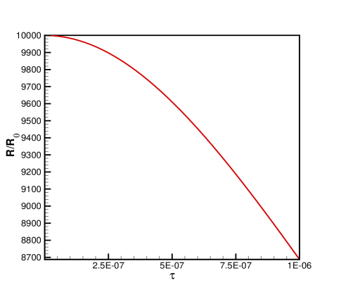
Figure 1: Dynamics of $y=R/R_{0}$ in terms of $\tau=tR_{0}^{1/2}$ for the radiation dominate epoch. This dynamics results from the metric formalism for the field equation. The action for the modified gravity is taken as $f(R)=\sqrt{R^{2}-R_{0}^{2}}$.

Here the Ricci scalar should be larger than $R_{0}$ but comparable with this term. This assumption implies that Ricci scalar should be smaller than $H^{2}$ at that time. From the FRW metric Ricci scalar is related to the Hubble parameter through: $R=6\dot{H}+12H^{2}$. Considering $R(t)$ as a small and constant perturbation due to the modified gravity, the differential equation for the scale factor is $\ddot{a}+\dot{a}^{2}=\epsilon a^{2}$. By a change of variable as $x=a^{2}$ and considering the initial condition of $a=0$ at $t=0$, the solution of the equation yields: $x(t)=A\sinh(\sqrt{\epsilon}t)$. Expanding this expression around $t=0$ results in $a(t)=Ct^{1/2}+\sigma t^{5/2}$, where $\sigma$ is a small value.

This deviation of the scale factor from $a\propto t^{1/2}$ depends on the Ricci scalar at the radiation epoch. Since $R$ and $R_{0}$ are in the order of $H_{0}^{-2}$, we expect that this model does not alter the dynamics of the early universe from that of Einstein-Hilbert action.

II.2 Palatini formalism

In the Palatini formalism, the connections are considered as independent variables, different than the Christoffel symbols of the metricsot06 . Varying the action with respect to both the metric and the connections the corresponding field equations are obtained as:

$$f^{\prime}(R)R_{\mu\nu}-\frac{1}{2}f(R)g_{\mu\nu}=\kappa T_{\mu\nu},$$ (16)

$$\nabla_{\lambda}(\sqrt{-g}f^{\prime}(R)g^{\mu\nu})=0,$$ (17)

in which we have considered the matter action to be independent of the connections. From equation(17) we can see that the connections are the Christoffel symbols of the new metric $h_{\mu\nu}$ where it is conformally related to the original one via the equation

$$h_{\mu\nu}=f^{\prime}(R)g_{\mu\nu}.$$ (18)

Equation (16) shows that in contrast to the metric variation approach (see equation 2), the field equations are second order in this formalism. The trace of field equations in the Palatini formalism for $f(R)=\sqrt{R^{2}-R_{0}^{2}}$ is:

$$\frac{R^{2}}{\sqrt{R^{2}-R_{0}^{2}}}-2\sqrt{R^{2}-R_{0}^{2}}=\kappa T.$$ (19)

The vacuum solution of this equation $R=\sqrt{2}R_{0}$, is the same as in the metric formalism. Through the conformal transformation of the metric $g_{\mu\nu}$ to $h_{\mu\nu}$, we get the corresponding Ricci tensor:

$$R_{00}=-3\frac{\ddot{a}}{a}+\frac{3}{2}f^{\prime-2}(\partial_{0}f^{\prime})^{2}-\frac{3}{2}f^{\prime-1}\bar{\nabla}_{0}\bar{\nabla}_{0}f^{\prime},$$ (20)

$$R_{ij}=[a\ddot{a}+2\dot{a}^{2}+f^{\prime-1}\left\{{}^{\lambda}_{\mu\nu}\right\}\partial_{0}f^{\prime}+\frac{a^{2}}{2}f^{\prime-1}\bar{\nabla}_{0}\bar{\nabla}_{0}f^{\prime}]\delta_{ij},$$ (21)

where $\left\{{}^{\lambda}_{\mu\nu}\right\}$ and $\bar{\nabla}$ are associated with $g_{\mu\nu}$. Using eqs. (16), (20) and (21) we can derive the modified Friedmann equation:

$$6H^{2}+6Hf^{\prime-1}\partial_{0}f^{\prime}+\frac{3}{2}f^{\prime-2}(\partial_{0}f^{\prime})^{2}=\frac{\kappa(\rho+3p)+f}{f^{\prime}}.$$ (22)

Now we want to obtain the dynamics of universe in the radiation dominant epoch. For this epoch implying the equation of state $p=1/3\rho$, from the equation (19) $T=0$, we get a constant value of $R_{r}=\sqrt{2}R_{0}$ for the Ricci scalar. Substituting it in (22) results in:

$$6H^{2}=\frac{2\kappa\rho_{r}+R_{0}}{\sqrt{2}}$$ (23)

in which the radiation density changes by the scale factor of the universe as $\rho_{r}=\rho_{0}a^{-4}$. The solution of equation (23) results:

$$a(t)\propto\sinh^{1/2}(\sqrt[4]{\frac{2R_{0}^{2}}{9}}t).$$ (24)

This solution is similar to the case of metric formalism, showing that for the action of $f(R)=\sqrt{R^{2}-R_{0}^{2}}$, we have almost the same dynamics for the early universe in both Palatini and metric formalism.

For the matter dominant epoch we use the direct dependence of the Hubble parameter and scale factor on $f(R)$ asama06 :

$$H^{2} = \frac{1}{6f^{\prime}}\frac{Rf^{\prime}-3f}{\left(1-\frac{3}{2}\frac{f^{\prime\prime}(Rf^{\prime}-2f)}{f^{\prime}(Rf^{\prime\prime}-f^{\prime})}\right)^{2}},$$ (25)

$$a = \left(\frac{1}{\kappa\rho_{0}}\left(Rf^{\prime}-2f\right)\right)^{-\frac{1}{3}}.$$ (26)

The numerical solution of these equations for $f(R)=\sqrt{R^{2}-R_{0}^{2}}$ gravity is shown in Fig. 2. Here we obtain the Hubble parameter normalized to its present value in terms of the scale factor, in logarithmic scale.

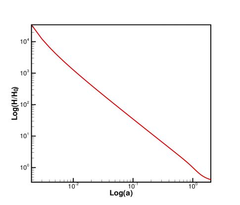
Figure 2: Numerical solution of Equations (25) and (26). Here we omit the Ricci scalar between the two equations and obtain a direct relation between the Hubble parameter and scale factor in the logarithmic scale.

By the numerical solution of H=H(a) a direct relation between the scale factor and cosmic time normalized to the $R_{0}^{-1/2}$ is shown in Fig. 3.

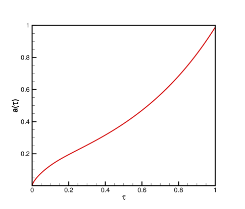
Figure 3: Numerical solution of scale factor in terms of cosmic time, normalized to the $R_{0}^{-1/2}$.

III Equivalence of the Modified gravity with scalar tensor theories

Here in this section we discuss the equivalence of the modified gravity with the scalar tensor theories, such as scalar-tensor coupled to the curvature like Brans-Dicke and non-minimally coupled one which is a result of conformal transformation from the Jordan to the Einstein framebrans . Here in this section we study the corresponding theories of $f(R)=\sqrt{R^{2}-R_{0}^{2}}$ action.

III.1 Brans-Dicke theory

Theories in which scalar fields are coupled directly to the curvature, are termed scalar-tensor gravity tey83 . Such theories can be found in the low-energy effective string theory which couples a dilation field to the Ricci curvature tensor. The simplest and the well known one is the Brans-Dicke (BD) theory. The BD theory is a generalization of the general relativity with the action of:

$$S_{BD}=\frac{1}{2\kappa}\int{d^{4}x\sqrt{-g}[\phi{R}-\frac{\omega_{0}}{\phi}(\partial_{\mu}\phi\partial^{\mu}\phi)-V(\phi)]}$$

$$+S_{M}(g_{\mu\nu},\psi),$$ (27)

where the free parameter $\omega_{0}$ is often called Brans-Dicke parameter and for the case of $\omega_{0}\rightarrow\infty$ GR is recovered. The field equation that one derives from the action (27) by varying with respect to the metric and the scalar field are

$$G_{\mu\nu}=\frac{\kappa}{\phi}T_{\mu\nu}+\frac{\omega_{0}}{\phi^{2}}(\nabla_{\mu}\phi\nabla_{\nu}\phi-\frac{1}{2}g_{\mu\nu}\nabla^{\lambda}\phi\nabla_{\lambda}\phi)$$ (28)

$$+\frac{1}{\phi}(\nabla_{\mu}\nabla_{\nu}\phi-g_{\mu\nu}\nabla_{\alpha}\nabla^{\alpha}\phi)-\frac{V}{2\phi}g_{\mu\nu}$$

$$\frac{2\omega_{0}}{\phi}\nabla_{\alpha}\nabla^{\alpha}{\phi}+R-\frac{\omega_{0}}{\phi^{2}}\nabla_{\alpha}\phi\nabla^{\alpha}\phi-V^{\prime}=0$$ (29)

where $G_{\mu\nu}=R_{\mu\nu}-\frac{1}{2}Rg_{\mu\nu}$ is the Einstein tensor and $T_{\mu\nu}=\frac{-2}{\sqrt{-g}}\frac{\delta S_{M}}{\delta g^{\mu\nu}}$ is the stress-energy tensor. We take the trace of Eq.(28) and combine it with Eq. (29) to omit R, which results in the differential equation for the dynamics of scalar field as:

$$(2\omega_{0}+3)\nabla_{\alpha}\nabla^{\alpha}\phi=\kappa T+\phi V^{\prime}-2V$$ (30)

We can also find an equivalent action for the BD theory with introducing a modified gravity as $f(R)$. Let us use an auxiliary field $\chi$ and write an equivalent action as:

$$S=\frac{1}{2\kappa}\int{d^{4}x\sqrt{-g}(f(\chi)+f^{\prime}(\chi)(R-\chi))}+S_{M}(g_{\mu\nu},\psi).$$ (31)

Varying with respect to $\chi$ leads to the equation $\chi=R$ if $f^{\prime\prime}(\chi)\neq 0$. By redefining the field $\chi$, $\Phi=f^{\prime}(\chi)$ and setting:

$$V(\Phi)=\chi(\Phi)\Phi-f(\chi(\Phi))$$ (32)

the action takes the form of

$$S=\frac{1}{2\kappa}\int{d^{4}x\sqrt{-g}(\Phi{R}-V(\Phi))}+S_{M}(g_{\mu\nu},\psi)$$ (33)

Comparison with the action in (27) reveals that we have an equivalent Brans-Dicke theory with $\omega_{0}=0$. In other words $f(R)$ theories are fully equivalent to a class of Brans-Dicke theories with vanishing kinetic term. For the case of our action, $f(R)=\sqrt{R^{2}-R_{0}^{2}}$ we can easily find the proper Brans-Dicke potential using equation (32):

$$V(\Phi)=R_{0}\sqrt{\Phi^{2}-1}$$ (34)

The Ricci scalar also depends on the scalar field by (see Fig.4):

$$R=V^{\prime}=R_{0}\frac{\Phi}{\sqrt{\Phi^{2}-1}}.$$ (35)

For the early universe with large Ricci scalar we have $\phi\rightarrow 1$ and for the accelerating epoch of the universe, $\phi\rightarrow\infty$ which results in $R\rightarrow R_{0}$. Substituting the potential in the Brans-Dicke action, the final form of the equivalent action with the modified gravity is:

$$S_{BD}=\frac{1}{2\kappa}\int{d^{4}x\sqrt{-g}(\Phi{R}-R_{0}\sqrt{\Phi^{2}-1})}+S_{M}(g_{\mu\nu},\psi)$$ (36)

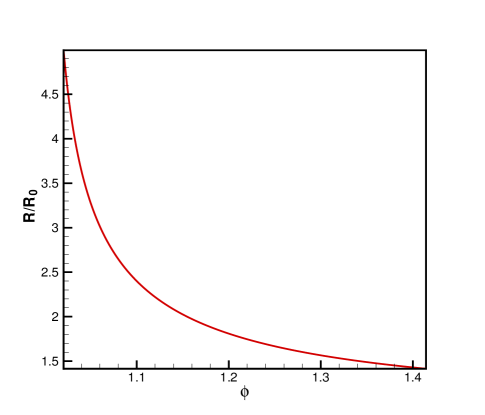
Figure 4: The dependence of the scalar field on the Ricci scalar in Brans-Dicke correspondence to the modified gravity.

III.2 Non-minimally coupled scalar-tensor gravity: conformal transformation

Metric theories of gravitation which depend on the scalar curvature in a nonlinear way, are usually called improperly nonlinear gravity (NLG) models mag93 . A suitable conformal transformation on metric can change the NLG lagrangian from the original frame so-called Jordan frame into Einstein-Hilbert one, minimally coupled to a scalar field. It is therefore claimed that any NLG theory is mathematically equivalent to General Relativity (with the scalar field), but from the physical point of view there is a debate in literature if there is an experiment to distinguish them mag93 .

To show the equivalence of these two frames one can use the auxiliary fields A and B and rewrite the action (1) as:

$$S=\frac{1}{2\kappa}\int{d^{4}x\sqrt{-g}(B(R-A)+f(A))}$$ (37)

Varying the action with respect to $B$ we get $R=A$ which results in generalized gravity in Jordan frame. Also varying the action with respect to $A$ we get $B=f^{\prime}(A)$ and we can write the action as:

$$S=\frac{1}{2\kappa}\int{d^{4}x\sqrt{-g}(f^{\prime}(A)(R-A)+f(A))}$$ (38)

Now we use the conformal transformation $g_{\mu\nu}\rightarrow\exp(\varphi)g_{\mu\nu}$ where $\varphi=-\ln{f^{\prime}(A)}$ and obtain the Einstein frame action (scalar-tensor gravity), as follows:

$$S=\frac{1}{\kappa^{2}}\int d^{4}x\sqrt{-g}[R-\frac{3}{2}[{\frac{f^{\prime\prime}(A)}{f^{\prime}(A)}}]^{2}{g^{\mu\nu}\partial_{\mu}A\partial_{\nu}A}$$

$$-\frac{A}{f(A)^{\prime}}+\frac{f(A)}{[{f^{\prime}(A)}]^{2}}].$$ (39)

We can also write this action as:

$$S=\frac{1}{\kappa^{2}}\int{d^{4}x\sqrt{-g}[R-\frac{3}{2}g^{\mu\nu}\partial_{\mu}\varphi\partial_{\nu}\varphi-V(\varphi)]}$$ (40)

where the scalar potential is:

$$V(\varphi)=\frac{A}{f^{\prime}(A)}-\frac{f(A)}{{f^{\prime}(A)}^{2}}$$ (41)

For the case of $f(R)=\sqrt{R^{2}-R_{0}^{2}}$, the potential of non-minimally coupled theory is:

$$\phi=\ln\frac{R}{\sqrt{R^{2}-R_{0}^{2}}},$$

$$V(\phi)=R_{0}e^{-\phi}\sqrt{1-e^{-2\phi}}.$$ (42)

where for convenience we changed $\varphi$ to $-\varphi$ in our calculation. For the early universe where $R\longrightarrow\infty$, $\phi\longrightarrow 0$ and for $R=R_{0}$ which is the vacuum solution of the generalized gravity, $\phi=\ln{\sqrt{2}}$. Figure (5) shows the dependence of the potential to the scalar field and the evolution of field starts from $\phi=0$ to its maximum value at $\phi=\ln{\sqrt{2}}$. The final stage of the scalar field results in de Sitter phase expansion of the universe.

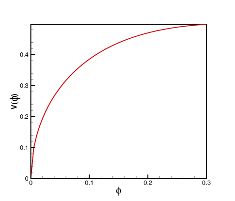
Figure 5: Dependence of potential on the scalar field results from the conformal transformation from Jordan to the Einstein frame in $f(R)=\sqrt{R^{2}-R_{0}^{2}}$ gravity.

IV Instability of $f(R)$ gravity

In order to examine the instability of the action we do a small perturbation of Ricci scalar around the vacuum solution to see if the perturbation grows or decays. A small perturbation around the vacuum can be written:

$$R=R_{v}+R_{1},$$ (43)

where $R_{1}\ll R_{v}$ and $R_{v}$ is the Ricci scalar of the vacuum. To find the dynamics of $R_{1}$, we expand the trace of Equation (2) around $R_{v}$ as:

$$f^{\prime}(R_{v}+R_{1})(R_{v}+R_{1})-2f(R_{v}+R_{1})+3\nabla^{\mu}\nabla_{\mu}f^{\prime}(R_{v}+R_{1})=0,$$ (44)

where the first order perturbation gives:

$$\nabla^{\mu}\nabla_{\mu}R_{1}+\frac{R_{v}f^{\prime\prime}(R_{v})-f^{\prime}(R_{v})}{3f^{\prime\prime}(R_{v})}R_{1}=0.$$ (45)

For the case of $f(R)=\sqrt{R^{2}-R^{2}_{0}}$, we have:

$$\nabla^{\mu}\nabla_{\mu}R_{1}+bR_{1}=0,$$ (46)

where $b=\frac{2\sqrt{2}}{3}R_{0}$. For FRW metric we can write this equation as follows:

$$-\ddot{R_{1}}+a^{-2}(t)(\partial^{2}_{x}+\partial^{2}_{y}+\partial^{2}_{z})R_{1}+bR_{1}=0.$$ (47)

Since the vacuum solution of the background results in a de Sitter solution and exponential expansion of the universe, we use $a(t)=\exp^{\frac{1}{2}\alpha(t-t_{0})}$ for the dynamics of the background, in which $\alpha=(\frac{\sqrt{2}R_{0}}{3})^{\frac{1}{2}}$. In the Fourier space (47) can be written as:

$$\ddot{R}_{1}(k)+k^{2}e^{-\alpha(t-t_{0})}R_{1}(k)-bR_{1}(k)=0.$$ (48)

It is clear that in the limit $t\rightarrow\infty$ we can ignore the second term and the solution is exponentially growing. We can also do semi-analytical calculation by using $\alpha\sim t_{0}^{-1}$ and $b\sim t_{0}^{-2}$ and as a result, the differential equation is:

$${R^{\prime\prime}}_{1}(k)+(e^{1-\tau}k^{2}-1)R_{1}(k)=0,$$ (49)

where prime represents derivation with respect to the dimensionless variable $\tau=\frac{t}{t_{0}}$. For perturbations smaller than horizon, (i.e. $k<1$) we will have exponentially growing modes, while wavelengths larger than horizon will oscillate. Figure (6) shows the dynamics of $R_{1}$ in terms of the normalized time $\tau$ for the modes smaller than horizon.

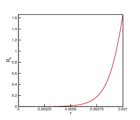
Figure 6: Numerical solution of Equation (49) for the perturbation of Ricci scalar around vacuum solution.

In order to stabilize this action we can add a quadratic term to the the action as $\alpha R^{2}$ and examine the stability. This stability condition can be also obtained if one directly solves the perturbed generalized Einstein equation:

$$-{R^{\prime\prime}_{1}}+e^{-(\tau-1)}(\partial^{2}_{x}+\partial^{2}_{y}+\partial^{2}_{z})R_{1}+bR_{1}=0,$$ (50)

where $b=\frac{2\sqrt{2}}{3}(R_{0}^{-1}-2\alpha)^{-1}$. For $\tau\ll 1$ and in the Fourier space, one gets

$$\ddot{R}_{1}(k)+(ek^{2}-b)R_{1}(k)=0.$$ (51)

So $R_{1}(k)$ would oscillate if $ek^{2}>b$, or equivalently, the model would be stable for perturbations of all wavelengths if

$$2R_{0}\alpha>1$$ (52)

Adding $\alpha R^{2}$ term not only makes the action stable but it will be also important for the early time inflation. To show this we can ignore the first term of action at the early universe while $R>>R_{0}$ and consider the action as:

$$f(R)\simeq\alpha R^{2}.$$ (53)

For the radiation dominant epoch where $p=1/3\rho$, the trace of energy momentum tensor is zero, $T^{\mu}{}_{\mu}=0$. So the generalized Einstein equation reduces to

$$\nabla^{\mu}\nabla_{\mu}f^{\prime}(R)=0.$$ (54)

For homogenous universe we will have only temporal derivative of $f^{\prime}(R)=2\alpha R$, which results in:

$$\nabla^{0}\nabla_{0}R=0,$$ (55)

where for FRW metric $\Gamma^{0}_{0\lambda}=0$ and we can replace the covariant derivatives with partial ones which results in:

$$R=Ct+D,$$ (56)

$C$ and $D$ can be chosen so that when $t\simeq 0$, $R\simeq D$. So the scale factor would behave exponentially ($a(t)\propto e^{\frac{\sqrt{D}}{2}t}$) in the very early epoch.

The same result can be achieved by looking to the instability of scalar potential of $V(\phi)$ in conformal transformation of metric to Einstein frame. For the case of $f(R)=\sqrt{R^{2}-R_{0}^{2}}$ the corresponding scalar potential as shown in Figure (5) is instable at the maximum of the potential since $V^{{}^{\prime\prime}}<0$. Adding the quadratic term gives the scalar potential as:

$$V(\phi(R))=\frac{R}{\frac{R}{\sqrt{R^{2}-R_{0}^{2}}}+2\alpha R}-\frac{\sqrt{R^{2}-R_{0}^{2}}+\alpha R^{2}}{(\frac{R}{\sqrt{R^{2}-R_{0}^{2}}}+2\alpha R)^{2}}.$$ (57)

Using the trace of generalized Einstein gravity, vacuum happens again at $R=\sqrt{2}R_{0}$. The second derivation of potential at $R=\sqrt{2}R_{0}$ yields:

$$V^{\prime\prime}(R=\sqrt{2}R_{0})=\frac{-1+4R_{0}^{2}\alpha^{2}}{R_{0}(1+2R_{0}\alpha)^{4}}.$$ (58)

The stability condition $V^{\prime\prime}>0$, implies $2R_{0}\alpha>1$, which is in agreement with (52), the approach of perturbation of Ricci scalar.

V Conclusion

Here in this work we introduced a new action for the gravity as $f(R)=\sqrt{R^{2}-R_{0}^{2}}$ which can imply a late time acceleration for the universe. Expanding this action results in $F(R)=R-1/2R_{0}^{2}/R+...$ which is similar to that of $1/R$ gravity models. In the strong gravity regime, action can be written as $f(R)=R$ and the Einstein-Hilbert action is recovered. By the two different metric and Palatini approaches we obtained the field equations of gravity and showed that by tuning the parameter of model $R_{0}$ , universe can enter an acceleration phase in any desired redshift.

We also obtained the equivalent theories as the Brans-Dicke and non-minimally coupled scalar-tensor gravity. Finally the instability of this action was examined by perturbing the Ricci scalar around the vacuum solution which showed that we have instability for the perturbations smaller than the horizon wavelength. Adding the quadratic term of $\alpha R^{2}$ to the action stabilize it for this type of perturbations for $2\alpha R_{0}>1$. We also tested the stability condition for the scalar field in the equivalent scalar-tensor gravity which resulted in $2\alpha R_{0}>1$.

Appendix

In Section II the solution of the generalized Einstein equation in the spherically symmetric space for the special case of vacuum solution is obtained. We try to find another solution perturbing Ricci scalar around the vacuum solution as:

$$R=\sqrt{2}R_{0}+f(r)\epsilon,$$ (59)

where $\varepsilon$ is a small dimensionless parameter. Substituting this term in the vacuum field equation of (4) and ignoring the terms of second order in $\varepsilon$ gives:

$$f(r)^{{}^{\prime\prime}}-\frac{2\sqrt{2}}{3}R_{0}f(r)=0,$$ (60)

where the solution is as:

$$f(r)=A\sin{(\sqrt{\frac{2\sqrt{2}R_{0}}{3}}r)}+B\cos{(\sqrt{\frac{2\sqrt{2}R_{0}}{3}}r)}.$$ (61)

We can ignore the ”sin” term by the argument that the maximum of Ricci scalar is around the gravitational source which should be vanished at infinity. So the overall Ricci scalar can be written as:

$$R=\sqrt{2}R_{0}+R_{0}\cos{(\sqrt{\frac{2\sqrt{2}R_{0}}{3}}r)}\varepsilon$$ (62)

Substituting the Ricci scalar in (9), we obtain the metric as:

$$\lambda(r)=-\ln[1+\frac{c_{1}}{r}-\frac{c_{2}}{r^{2}}-\frac{\sqrt{2}}{12}R_{0}r^{2}$$ (63)

$$-R_{0}\varepsilon[\frac{1}{r^{2}}\int{r^{3}\cos{(\frac{1}{3}2^{\frac{3}{4}}\sqrt{3R_{0}}r)}}dr$$

$$-r\int{r^{2}\cos{(\frac{1}{3}2^{\frac{3}{4}}\sqrt{3R_{0}}r)}}dr]]$$

It is obvious that if we set $\varepsilon=0$ (ignore the perturbation term) we will achieve the solution of constant Ricci scalar and we can determine $c_{1}=-2GM/c^{2}$ and $c_{2}=0$ .

Acknowledgements We would like to thank M. M. Sheikh Jabbari for his useful comments in this work.

References

References

- (1) C. L. Bennett et al., Astrophys. J. Suppl. 148, 1 (2003).
- (2) C. B. Netterfield et al. [Boomerang Collaboration], Astrophys. J. 571, 604 (2002).
- (3) N. W. Halverson et al., Astrophys. J. 568, 38 (2002).
- (4) A. G. Riess et al., Astrophys. J. 607, 665 (2004).
- (5) S. Perlmutter et al. [Supernova Cosmology Project Collaboration], Astrophys. J. 517, 565 (1999).
- (6) J. L. Tonry et al., Astrophys. J. 594 (2003).
- (7) S. M. Carroll, Living Rev. Rel. 4, 1 (2001).
- (8) P. J. E. Peebles and R. Ratra, Rev. Mod. Phys. 75, 599 (2003).
- (9) P. J. E. Peebles and R. Ratra, Astrophys. J. 325, L17 (1988).
- (10) C. Wetterich, Nucl. Phys. B 302, 668 (1988).
- (11) V. Sahni and A. Starobinsky, Int. J. Mod. Phys. D 9, 373 (2000).
- (12) C. Armendariz-Picon, V. Mukhanov and P. J. Steinhardt, Phys. Rev. Lett. 85, 4438 (2000).
- (13) J. S. Bagla, H. K. Jassal and T. Padmanabhan, Phys. Rev. D 67, 063504 (2003).
- (14) R. R. Caldwell, Phys. Lett. B 545, 23 (2002).
- (15) R. R. Caldwell, M. Kamionkowski and N. N. Weinberg, Phys. Rev. Lett. 91, 071301 (2003).
- (16) C. Wetterich, Physics Lett. B 594, 17 (2004).
- (17) M. S. Movahed and S. Rahvar, Phys. Rev. D 73, 083518 (2006).
- (18) C. Armendariz-Picon, T. Damour and V. Mukhanov, Phys. Lett. B 458, 209 (1999).
- (19) L. Mersini, M. Bastero-Gil and P. Kanti, Phys. Rev. D 64, 043508 (2001).
- (20) S. M. Carroll, M. Hoffman and M. Trodden, Phys. Rev. D 68, 023509(2003).
- (21) L. Parker and A. Raval, Phys. Rev. D 60, 063512 (1999).
- (22) T. Clifton , J. Barrow , Phys. Rev. D 72, 103005 (2005).
- (23) S. Nojiri and S. D. Odintsov, Phys. Rev. D 68, 123512 (2003).
- (24) S. Nojiri and S. D. Odintsov, Phys. Lett. B 562, 147 (2003).
- (25) C. Deffayet, G. R. Dvali and G. Gabadadze, Phys. Rev. D 65, 044023 (2002).
- (26) K. Freese and M. Lewis, Phys. Lett. B 540, 1 (2002).
- (27) M. Ahmed, S. Dodelson, P. B. Greene and R. Sorkin, Phys. Rev. D 69 103523(2004) .
- (28) N. Arkani-Hamed, S. Dimopoulos, G. Dvali and G. Gabadadze, hep-th/0209227.
- (29) G. Dvali and M. S. Turner, Fermilab pub. 03040-A (2003).
- (30) R. Brandenberger and G. Gheshnizjani, Phys. Rev. D 66 123507 (2002).
- (31) R. Mansouri, astro-ph/0512605.
- (32) S. Pireaux, J. P. Roselot and S. Godier, Astro-phy. Space Sci. 284 1159 (2003).
- (33) G. V. Kraniotis and S. B. Whitese, Class. Quant. Grav. 20 4817 (2003).
- (34) M. Amarzguioui et al. A&A 454, 707 (2006).
- (35) T. P. Sotiriou, gr-qc/0604006.
- (36) T. P. Sotiriou, Class. Quant. Grav. 23 5117 (2006).
- (37) P. Teyssandir and P. Tourrence, J. Math Phys. 24 2793 (1983).
- (38) G. Magnano and L. M. Sokolowski, Phys. Rev. D 505039 (1994).