Constraining quasar host halo masses with the strength of nearby Lyman-alpha forest absorption

Abstract

Using cosmological hydrodynamic simulations we measure the mean transmitted flux in the Ly$\alpha$  forest for quasar sightlines that pass near a foreground quasar. We find that the trend of absorption with pixel-quasar separation distance can be fitted using a simple power law form including the usual correlation function parameters $r_{0}$ and $\gamma$ so that ($\left<F(r)\right>=\sum\exp(-\tau_{\rm eff}(1+(\frac{r}{r_{0}})^{-\gamma}))$). From the simulations we find the relation between $r_{0}$ and quasar mass and formulate this as a way to estimate quasar host dark matter halo masses, quantifying uncertainties due to cosmological and IGM parameters, and redshift errors. With this method, we examine data for $\sim 3000$ quasars from the Sloan Digital Sky Survey (SDSS) Data Release 3, assuming that the effect of ionizing radiation from quasars (the so-called transverse proximity effect) is unimportant (no evidence for it is seen in the data.) We find that the best fit host halo mass for SDSS quasars with mean redshift $z=3$ and absolute G band magnitude $-27.5$ is $\log_{10}{\rm M/{\rm M_{\odot}}}$=$12.48^{+0.53}_{-0.89}$. We also use the Lyman-Break Galaxy (LBG) and Ly$\alpha$  forest data of Adelberger et al in a similar fashion to constrain the halo mass of LBGs to be $\log_{10}{\rm M/{\rm M_{\odot}}}$=$11.13^{+0.39}_{-0.55}$, a factor of $\sim 20$ lower than the bright quasars. In addition, we study the redshift distortions of the Ly$\alpha$  forest around quasars, using the simulations. We use the quadrupole to monopole ratio of the quasar-Ly$\alpha$  forest correlation function as a measure of the squashing effect. We find that this does not have a measurable dependence on halo mass, but may be useful for constraining cosmic geometry.

1 Introduction

The Lyman-alpha forest of absorption lines seen in the spectra of quasars see (e.g., Rauch 1998 for a review) can be related in theories of structure formation to fluctuations in the matter distribution. Because the fluctuations are only weakly non-linear, the photoionized gas where they arise traces the dark matter distribution that dominates the gravitational potential very well, and the Ly$\alpha$  forest can be used to give us information on structure in the dark matter (e.g., Cen et al. 1994; Zhang, Anninos, & Norman 1995; Petitjean, Mücket, & Kates 1995; Hernquist et al. 1996; Katz et al. 1996; Wadsley & Bond 1997; Theuns et al. 1998; Davé et al. 1999). We can therefore use the Ly$\alpha$  forest absorption around galaxies and quasars to tell us about the profile of dark matter around these objects. The clustering of dark matter around dark matter halos is expected to be related to their mass. This has been used by e.g., Seljak et al. (2005) and Mandelbaum et al. (2006), to constrain the mass of galaxy halos using the matter distribution around them inferred from weak lensing observations. In the present paper, we propose to infer related constraints on the mass of quasar hosts and high redshift galaxies from the Ly$\alpha$  forest-derived mass profiles around them.

Some current mass constraints for quasar hosts and high redshift galaxies come from considering the amplitudes of their two point-correlation functions. For example, Croom et al. 2005 analyzed the autocorrelation function of quasars in 2dF data, and Myers et al. (2006) the clustering of 300,000 photometrically classified SDSS QSO to find constraints on quasar host masses.

It has been known since the work of Bajtlik et al. (1988) that the Ly$\alpha$  forest in the spectrum of quasars shows evidence of decreasing absorption as the quasar’s emission redshift is approached. This is known as the proximity effect, and is believed to be due to photoionization from the quasar itself adding to the mean background photoionizing radiation field and decreasing the amount of neutral hydrogen in the vicinity of the quasar. Knowing quasar observed luminosities, the observed decrease in Ly$\alpha$  absorption has been used to estimate the intensity of the mean cosmic background photoionizing radiation field (see e.g., Scott et al. 2000). A related process is the possible effect of other (foreground) quasars on the Ly$\alpha$  forest of other quasars whose sightlines pass close by. This effect, known as the transverse, or foreground proximity effect has not so far been observed, and in fact there have been several non-detections of the effect (e.g. Schirber & Miralda-Escude 2004, Croft 2004 ).

This could be explained if for example quasar radiation is beamed, so that the usual proximity effect would occur but off-axis sightlines would not be affected. Alternatively, the quasar lifetime could be short enough that light has not had time to travel transversely to adjacent sightlines (for example if they are 10$\;h^{-1}{\rm Mpc}$ away, a quasar lifetime $\lower 2.15277pt\hbox{$\;\buildrel<\over{\sim}\;$}10$ Myr would leave them unaffected. The two studies referred to above point instead to increased Ly$\alpha$  absorption in the parts of sightlines that pass close to foreground quasars. This is expected, as quasars should be hosted by massive dark matter halos which are in overdense regions. We will use this fact along with theoretical predictions in the context of the Cold Dark Matter model to constrain the quasar halo masses. The same can also be done for high redshift galaxies where the quasar sightlines pass close to galaxies. Here the proximity effect is known definitively to be too small to affect the spectra (see e.g. Bruscoli et al. 2003) and instead increased absorption is also seen (Adelberger et al. 2003). Some related work on the Ly$\alpha$  optical depth around quasars has been carried out by Rollinde et al. 2005 and the distribution of damped Ly$\alpha$  absorption around foreground quasars by Hennawi et al. (2006).

Looking at the profile of Ly$\alpha$  forest absorption around quasars in two dimensions, one parallel and one perpendicular to the line of sight allows one to quantify redshift distortions. As the gravitating mass governs the amount of squashing seen (e.g., Kaiser 1987, Regos & Geller 1989), measuring it may allow us to infer the mass enclosed within a given radius in a complementary way to looking at the mean strength of Ly$\alpha$  absorption.

Our plan for the paper is as follows: In §2, we describe the hydrodynamic simulations we used, as well as how Ly$\alpha$  spectra were made. In this section we also compute the mean density and velocity profiles as a function of halo mass, directly from the simulation mass and velocity data. We also compute the mean Ly$\alpha$  forest flux as a function of quasar-pixel distance, for different mass bins. In §3 we describe how we fit the Ly$\alpha$  forest flux-distance trend with a simple power-law model and how the power law parameters depend on the halo mass. In §4 we describe the data from the SDSS and the LBG data from Adelberger and use our results from §3 to constrain the halo masses. In §5, we examine the redshift space anisotropy of clustering. In §6 we discuss our results and conclude.

2 Simulated QSO spectra

2.1 Simulations

We use two large N-body + hydrodynamics simulations of a $\Lambda$ CDM cosmology to make our spectra. The two simulations were run using the code GADGET-2 (Springel, Yoshida & White 2001, Springel 2005), and are described more fuly in Nagamine et al. 2005. The simulations have the same cosmological parameters ( $\Omega_{\Lambda}=0.7,\Omega_{m}=0.3,\Omega_{b}=0.04$ and $H_{0}=70{\rm\;km\;s^{-1}}\;{\rm Mpc}^{-1}$, $\sigma_{8}$=0.9) but have different box sizes and particle numbers. This means that they have significantly different mass and spatial resolutions so that we can use them for a resolution study, in order to make sure that our results have converged. Both simulations include gas physics, heating, cooling, a prescription for star formation (Springel & Hernquist 2003) and the effect of stellar feedback on has properties.

One simulation is the G6 run, a cubic box of 100 $\;h^{-1}{\rm Mpc}$ on each side, with $486^{3}$ dark matter particles and $486^{3}$ gas particles. This results in an initial mass per gas particle of $9.7\times 10^{7}{\rm M_{\odot}}$ and dark matter mass $6.3\times 10^{8}{\rm M_{\odot}}$. The other is the D5 run, a cubic box of side length $33.75\;h^{-1}{\rm Mpc}$ and $2\times 324^{3}$ particles.

2.2 Mock spectra

We use simulation outputs from redshift $3$ to make mock Ly$\alpha$  spectra. This was done in the usual manner, by integrating through the SPH kernels of the particles to obtain the neutral hydrogen density field, and then convolving with the line of sight velocity field (see e.g., Hernquist et al. 1996) The mean UV background radiation intensity has been normalized so that the spectra have a mean effective optical length $\tau_{\rm eff}=0.4$ (where $\tau_{\rm eff}=-\ln\left<F\right>$) or equivalently a mean flux $\left<F\right>$=0.67. We make 5000 spectra from each simulation, where the sightlines are parallel to the box axes and the $x-y$ positions of the sightlines are picked randomly.

2.3 Quasar hosts

For halo finding, we use the friends-of-friends (fof) method (e.g., Huchra & Geller 1982). A particle is defined to belong to a group if it is within some linking length ($b$) of any other particle in the group. We select clusters by using $b=0.2$ where $b$ is the linking length as a fraction of the mean particle separation. This definition of dark matter haloes was shown by Jenkins et al. (2001) to yield a mass function with a univeral form. We use these dark matter halos as our quasar hosts in the simulation. We bin the quasar hosts in terms of their mass. For each simulation we use has 5 mass bins, logarithmically spaced. There are 4 overlapping bins. D5 (G6) has one more bin smaller (larger) than the other 4. This is because in the D5 simulation there are too few halos with masses $>10^{12}{\rm M_{\odot}}$ and in the G6 simulation the mass per particle is too large to resolve halos with masses $<10^{9}{\rm M_{\odot}}$.

2.4 Mean baryonic density and infall velocity as a function of quasar-pixel distance

The baryonic density around quasars is related to the amount of neutral hydrogen which absorbs light via the Ly$\alpha$ energy transition. As we have mentioned in §1, baryons fall into gravitational wells formed by dark matter, and so the baryonic distribution will mimic that of dark matter. With two quasars with close angular positions, but at different redshifts, we can therefore investigate the distribution of dark matter by studying the Ly$\alpha$ absorption lines around a foreground quasar. Quasars have high luminosities despite their high redshift, and so allow us to probe the high redshift Universe.

Because the density profile around quasars in the simulation is directly available to us from the simulation data, we examine this first, before moving on to study the Ly$\alpha$  absorption profile. In order to compute the baryonic density profile, we loop over all quasars in a mass bin and all pixels in the spectra. For each quasar-pixel pair we compute the separation, $r$ in comoving $\;h^{-1}{\rm Mpc}$. We average the density values for all pairs at a given separation and show the results in Figure 1.

We naturally expect that the baryonic density should be a decreasing function of r and that the overall amplitude should monotonically increase as the quasar host mass increases (Figure 1.) We find that this is generally the case, except for the fact that the the smallest mass bin in each simulation shows a higher density profile amplitude than expected (we will see later that this also the case for the mean flux profile). When we look at the overlap region for the two simulations we will see later that this is clearly a resolution effect. For the bins in quasar host mass which are well resolved in the two simulations there is good agreement.

Figure 1: Baryonic density in units of the cosmic mean as a function of $r$ (distance from a dark matter halo) in real space for the D5 simulation(top) and G6 simulation (bottom). We show results for different dark matter halo masses.

We also compute the mean infall velocity as a function of quasar-pixel separation. The infall velocity ($v_{\rm infall}$)is defined as the velocity component pointing towards the center of a quasar host. It should depend on the gravitational pull of the mass surrounding a quasar and therefore decrease as $r$ does and increase as quasar host halo mass increases (Figure 2). The tangential component will add up to zero if we average over the velocity of gas around a quasar. As seen in the case of the baryonic density, the resolution effect may be responsible for some mass bins having higher $v_{infall}$ than predicted. There is discrepancy between the two runs for the same mass bin on large $r$ scales. This is likely to be because the box size of the D5 run is much smaller and peculiar velocities are sensitive to large-scale density fluctuations.

Figure 2: Infall velocity as a function of $r$ in real space for the simulations D5 (left) and G6 (right). Note that the plot scales are different because of different simulation size. The $v_{\rm infall}$ curve for the largest mass bin $\left<M\right>=2.9\times 10^{10}$ in the D5 simulation is shown as bold lines with crosses.

2.5 Mean Ly$\alpha$  forest flux as a function of quasar-pixel distance

For each mass bin, we calculate the mean absorbed flux defined as:

$$\left<F(r)\right>=\sum\exp^{-\tau(r)},$$ (1)

where $\tau(r)$ is the optical depth for Ly$\alpha$  absorption in redshift space, in a pixel at comoving distance from the quasar $r$. The observed flux is the fraction of photons with a given wavelength that are left unabsorbed by neutral hydrogen. Since the Ly$\alpha$ absorption should reflect the presence of neutral hydrogen, we expect the observed flux to be correlated with the baryonic density, which increases close to quasars (small quasar-pixel separation $r$) as shown in the previous section.

We use will use the G6 run, averaging over 500 spectra in this section as its mass resolution is suitable for the halo mass range relevant for quasars. We plot the mean flux in Figure 3 where we see that the flux asymptotically approaches a mean value on large scales, which is 0.67 in this case, the value set in the simulation. The bottom panel of Figure 3 shows the case when we add a Gaussian redshift error of 150 ${\rm\;km\;s^{-1}}$ to the quasar position. This is to reflect the measurement errors on observational determination of the quasar redshift. We can see that in this case, the shape of F(r) is different on small scales, $r<1\;h^{-1}{\rm Mpc}$ and also scatters more, especially for smaller mass halos. Since this is the G6 run, it may not be accurately reflecting the behaviour of quasar hosts of small mass in any case. On larger scales, which will be relevant for our fitting later, there is not much change.

The plot shows that the overall flux level $F(r)$ decreases with mass, because more baryonic matter near QSOs means more absorptions of photons by the Ly$\alpha$  forest, which results in less observed flux. As with the baryonic density (Figure 1) , we see that the smallest mean flux is not from the smallest mass bin. However, we expect this to be due to resolution effects. Apart from this, there is a good correlation between absorption and halo mass.

Figure 3: The mean transmitted flux in the Ly$\alpha$  forest in redshift space, as a function of quasar-pixel distance. Top: no redshift error has been added. Bottom: a Gaussian redshift error of 150 ${\rm\;km\;s^{-1}}$ has been added. The flux asymptotically approaches $\left<F\right>$=0.67, the mean value that has been set in the simulation.

2.6 Mean flux as a function of quasar-pixel separation perpendicular and parallel to the line of sight

The flux in redshift space is subject to redshift distortions because of peculiar velocities, which act in a way similar to their effect on the autocorrelation function (Kaiser 1987). The baryons around a quasar will infall towards it because of the gravity from the overdense region. This will result in the compression of the flux profile in the line of sight direction. The squashing effect will be greater for quasars with of larger host mass as they are associated with larger density fluctuations. We decompose the quasar-pixel separation $r$ into the transverse($\sigma$) and line of sight ($\pi$) directions ($r^{2}=\sigma^{2}+\pi^{2}$) and plot the flux as a function of these two parameters in Figure 4. Although its dependence on quasar mass is not very obvious, the distortion effect is clearly seen.

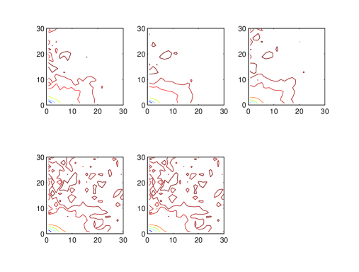
Figure 4: The mean observed flux in terms of transeverse and line of sight directions. The flux goes through redshift distortions due to peculiar velocities and looks squashed in the LOS direction. From the top left: $5.1\times 10^{9}~{}{\rm M_{\odot}},2.9\times 10^{10}~{}{\rm M_{\odot}},1.6\times 10^{11}~{}{\rm M_{\odot}},9.1\times 10^{11}~{}{\rm M_{\odot}}$ and $5.1\times 10^{12~{}}{\rm M_{\odot}}$.

In §5, we measure the anisotropy of the flux from simulations in redshift space by using Hamilton’s formulae (1992) to quantify it and compare it with observational data.

3 Fit to the Observed Flux vs quasar-pixel separation trend

In this section we parameterise $F(r)$ using $r_{0}$ and $\gamma$ which are commonly used in the power-law auto correlation function regularly applied to galaxy clustering data. Our aim is to eventually estimate the mass of SDSS quasar host halos and of Lyman Break Galaxy halos by using the relation between the fitted values of $r_{0}$ and halo masses.

We use 5000 spectra from the G6 run, computing the mean flux as a function of $r$ for 5 different mass bins. To fit the $F(r)$ we need to use a covariance matrix, as the bins are correlated. In order to make a covariance matrix, we divide the simulation box into 125 subvolumes. We calculate a full covariance matrix ($\sigma_{ij}^{M}$) from the mass bin that has most quasars. For the rest of mass bins there are not enough quasars to compute a covariance matrix that is noiseless enough to invert. Instead we infer the full covariance matrix by scaling up from the matrix computed from large number of quasars, making use of the diagonal elements, which can be calculated. We assume that the relative cross-correlations are the same for each covariance matrix. We therefore only calculate the diagonal elements ($\sigma_{ii}^{m}$) directly and calculate the off-diagonal elements from $\sigma_{ij}^{M}$ in the following way:

$$\sigma_{ij}^{m}=\sigma_{ij}^{M}\frac{\sqrt{\sigma_{ii}^{m}}\sqrt{\sigma_{jj}^{m}}}{\sqrt{\sigma_{ii}^{M}}\sqrt{\sigma_{jj}^{M}}}.$$ (2)

We use the mean flux as a function of quasar-pixel difference computed for 5 different mass bins. We then make curves for a total of 80 mass bins (18 bins in-between each) by linear interpolation. We also build a covariance matrix accordingly for each sub-mass bin, so that we can compute a smooth trend of fit parameters with mass.

3.1 F(r) fit as a function of halo mass

In order to find an equation that best describes $F(r)$, we try a power law form that is commonly used to fit the two point correlation function:

$$F(r)=\exp\left[-\tau_{\rm eff}\left(1+\left(\frac{r}{r_{0}}\right)^{-\gamma}\right)\right]$$ (3)

This formula describes the mean flux as an increasing function with $r$ that asymptotically approaches a certain value (because there will be no relative enhancement of neutral hydrogen far from a quasar). As $r$ becomes large, the second term in the exponent will decrease, leaving the the flux close to $\exp^{-\tau_{\rm eff}}$ which is the asymptotic value, and when $r$ r is small, Ly$\alpha$ absorption depends strongly on the distribution of matter around a quasar.

Figure 5: The mean flux as a function of quasar-pixel distance from the G6 simulation (symbols) and fits using equation 3 (lines.)

The value of $\tau_{\rm eff}$ is set so that the asymptotic value of equation 3 matches the one from the simulation. We fit the observed flux from the G6 simulation to equation 3 and show the results in Figure 5. These results show that even though it is very simple, equation 3 gives a very good description of the observed mean flux as a function of scale, at least for the $r$ range of interest.

We have fitted $r_{0}$ and $\gamma$ for the 80 mass bins, carrying out a $\chi^{2}$ analysis using the full covariance matrix built as explained previously. Figure 6 shows the best fit values of $r_{0}$ and $\gamma$ for the D5 and G6 simulations as a function quasar mass. Both $r_{0}$ and $\gamma$ decrease at first and then go up, which is consistent with the non-monotonic behaviour of the mean flux in terms of mass as shown in Figure 3. As we mentioned before, this is due to resolution effects, as we can see by for example examining what happens to halos which approach the resolution limit of the G6 simulation, and compare them to the well resolved D5 halos of the same mass.

We see that the slope is getting steeper when quasar mass increases, which implies that the overall amplitude of the flux on small scales decreases faster. Since the G6 run is more suited to the mass range of quasar hosts, we use the $r_{0}$-mass trends from this run in our fitting , although our conclusions are not sensitive to this.

We also carry out the same fitting procedure with the G6 run, after a Gaussian redshift error with $\sigma=150{\rm\;km\;s^{-1}}$ is added to the quasar redshifts. Both $r_{0}$ and $\gamma$ decrease with the addition of the redshift errors (also shown in Figure 6). The $r_{0}$ value is not much affected by the redshift errors, however.

Figure 6: The best fit $r_{0}$ and $\gamma$ fitted to the quasar host-Ly$\alpha$  forest profile vs. quasar host halo mass.

3.2 Application to observational data

Our next step is use the $r_{0}$-mass relation to estimate the mass of dark matter halos for quasars observed in the SDSS, and LBGs, both at redshift $z=3$. We will use equation 3 to find the $r_{0}$ and $\gamma$ values that best describe the mean flux as a function of separation and then use the best fit $r_{0}$ to estimate the mass.

4 Estimated Mass Limit for SDSS quasars

We use $\sim$3000 observed quasars from SDSS data release 3 (Abazajian et al. 2005), the subset of the total data that have redshifts $z>2.4$. This results in a mean redshift for the Ly$\alpha$  forest pixels used in our analysis of $z=3.0$, matched to the simulations we have been using. This quasar sample is rather bright, with mean $G$ magnitude -27.5. It would be ideal to have many pairs of close-by quasars but unfortunately they are rare in observations. Of the $3000$ quasars, only $\sim 100$ are close enough to contribute to the $F(r)$ for $r<20\;h^{-1}{\rm Mpc}$. In order to compute $F(r)$, the pixels in the SDSS spectra we convert the pixel redshifts and quasar positions into comoving cartesian coordinates assuming a $\Lambda$ CDM cosmology and then compute quasar-pixel separations. Only foreground quasars are used in our analysis, so that we are not sensitive to the regular proximity effect. The procedure is the same as in Croft (2004), where it is outlined in more detail.

The results for $F(r)$ for the SDSS quasars are shown in Figure 7, along with the best fit power law curve and jackknife error bars. In order to carry out the fit, we use the covariance matrix derived from the simulations, scaled so that the diagonal elements are the same as the observational error bars.

Using the $r_{0}$ vs. mass trend for the G6 simulation, we find the estimated mass for SDSS quasars host dark matter halos is $\log{\rm M/{\rm M_{\odot}}}$=$12.34^{+0.41}_{-0.73}$. Although not used in the analysis directly, fitting $\gamma$ helps narrow down the quasar mass. We also tried fixing a $\gamma$ (not necessarily the best fit value) and varied only $r_{0}$ but could not recover a mass limit. In the case of the Gaussian error of 150 ${\rm\;km\;s^{-1}}$, added to the quasar redshifts, the estimated mass limit becomes $\log{\rm M/{\rm M_{\odot}}}$=$12.48^{+0.41}_{-0.73}$. The result agrees well with that when the redshift error is not included, making the best fit mass slightly larger, by $\sim 20\%$. Given the large error bars on the halo mass, this is not significant.

The details of quasar formation and evolution in time are still in debate, which makes it difficult to predict the mass of quasar hosts, and there are few estimates their these masses from observational data. Wyithe & Padmanabhan (2006) report that mass estimates of quasar host dark matter haloes are from $10^{11}{\rm M_{\odot}}-10^{13}{\rm M_{\odot}}$, depending on the time-dependence of their evolution. Our value lies within this range of results.

4.1 Estimated Mass Limit for Lyman Break Galaxies

We apply our method to Lyman Break Galaxy data (Adelberger et al. 2003). The reported mass of LBGs from other methods at $z=2.9$ is $10^{11.2}-10^{11.8}$ (Adelberger et al. 2005) while other groups have slight different estimates: $10^{11.6\pm 0.3}{\rm M_{\odot}}$ (Weatherley & Warren 2005) and $10^{11.3}{\rm M_{\odot}}$ (Somerville et al. 2001).

The fitting procedure is same as previously used except that we ignore the the first three bins because the data for small $r$ is not consistent with the trend in the simulation despite the large error bars(Figure 8). If the data points are valid, it would need further investigation, and indeed these results may be indicative of starburst winds disturbing the Ly$\alpha$  forest on small scales. But for simplicity, and because winds from galaxies are unlikely to propagate far, we only use regions greater than 1.5$\;h^{-1}{\rm Mpc}$ in our analysis. We fit the LBG data to the equation 3 and then estimate the mass using the $r_{0}$-mass relation found in §3.1. The estimated mass of LBGs we find is $\log{\rm M/{\rm M_{\odot}}}$=$11.13^{+0.18}_{-0.23}$. The best fit value of mass is consistent with Adelberger’s estimate.

Figure 7: The mean transmitted flux as a function of quasar-pixel distance, for SDSS DR3 quasars (crosses with error bars) fitted with Eqn. 3 (dotted lines).

Figure 8: The mean flux of Adelberger’s data (crosses with error bars) fitted to Eqn. 3 (dotted lines)

4.2 Dependence on cosmological parameters

Figure 9: $r_{0}$ and $\gamma$ vs. quasar mass for different $\sigma_{8}$ values.(0.7, 0.9, and 1.1) No hydrodynamics is included in the simulation. No redshift error has been added.

In carrying out our analysis and computing constraints on the halo masses of quasars and LBGs we have assumed that the $r_{0}$- mass relation from the simulations applies to the observations. This is probably a valid assumption, as the cosmological model used in our simulation is close to that found from for example the WMAP satellite data (Spergel et al. 2003, 2006). As the error bars on our best fit quasar halo mass are large, we expect errors on cosmological parameters to have relatively little effect. In order to verify this, we vary the least constrained parameters, the amplitude of mass fluctuations, $\sigma_{8}$, running new simulations with different amplitudes and seeing if we get the same quasar host masses if we use these to compute the $r_{0}$-mass relation.

The new simulations are of dark matter only, and it is assumed that the gas traces the dark matter distribution. Three runs are made, with $\sigma_{8}$=0.7, 0.9 and 1.1. They are run in a 50 $\;h^{-1}{\rm Mpc}$ box, using $256^{3}$ particles. Spectra are made from the dark matter distributions in the manner described by e.g. Croft et al. (1998). Although the simulations do not include any hydrodynamics we expect the relative values of $r_{0}$ for the different $\sigma_{8}$ runs to closely approximate the values that would be obtained with full hydro simulations.

The fitting procedure is the same as the D5/G6 simulation cases except that the covariance matrix was built from 27 subvolumes because the simulation size is smaller than the G6 run. We fit the quasar data from SDSS using equation 3 and find the mass limits using the newly found $r_{0}$ vs. mass relation. We use no redshift error in the analysis. We find the mass limits as follows: $\log{\rm M/{\rm M_{\odot}}}$=$12.21^{+0.36}_{-0.54}$, $\log{\rm M/{\rm M_{\odot}}}$=$12.88^{+0.48}_{-0.91}$, and $\log{\rm M/{\rm M_{\odot}}}$=$12.68^{+0.41}_{-0.75}$ for $\sigma_{8}$ = 0.7, 0.9, and 1.1 respectively. The comparison with the results in §3.1 ($\log{\rm M/{\rm M_{\odot}}}$=$12.34^{+0.41}_{-0.73}$) indicates that the mass fluctuations do not have a significant effect on estimating quasar masses, at least within our error bars (less than a $1\sigma$ effect).

4.3 Dependence on $\tau_{\rm eff}$ and temperature

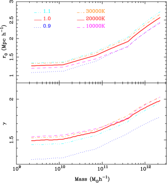
Figure 10: $r_{0}$ and $\gamma$ vs. quasar mass when mean observed fluxes are 90 and 110 % of the nominal value (0.67) and the gas temperature is 10,000K and 30,000K. The solid bold lines represent $\left<F(r)\right>$ =0.67 and T=20,000K case ($\sigma_{8}$=0.9) No hydrodynamics is included in the simulation. No redshift error has been added.

The hydrodynamic simulations have a gas temperature at the mean density close to 20,000 K (see observational determinations by e.g. Schaye et al. 2000) and mean effective optical depth ($\tau_{\rm eff}=-\ln\left<F\right>$)= 0.4, which has been set to be consistent with observational data. Both of these quantities have uncertainties, and these may affect our recovery of the quasar dark matter halo mass from Ly$\alpha$  forest clustering. We use the dark matter only simulation to estimate what the total errors on halo mass will be by quantifying the effect of changes in these parameters. We make Ly$\alpha$  spectra from the simulation setting $T_{0}=10,000$ K and 30,000 K instead of 20,000K. We also make spectra by changing the the mean flux $\left<F\right>$ by $\pm 10\%$ from our original value of $\left<F\right>=0.67$ In these cases the mean transmitted flux becomes 0.603 and 0.737, which translates to mean effective optical depths $\tau_{\rm eff}$ of 0.305 and 0.506, respectively. This range of $\tau_{\rm eff}$ covers the values measured by $\tau_{\rm eff}$ by Rauch et al. (1997) and other observed values: For example McDonald et al. (2000) reported $\tau_{\rm eff}$ $0.380\pm 9$% at z=3 and Schaye et al. (2003) obtained $\left<F\right>=0.696$ at z=3. Although we vary $\left<F\right>$ by $\pm 10\%$, this range is much larger than the scatter in the observed values, which we conservatively estimate to be $\pm 5\%$ at the 1 $\sigma$ level. We use this value when we compute the effect of $\left<F\right>$ uncertainty on the quasar host halo mass.

The fitting procedure is the same as in the previous sections. Figure 10 shows the mass vs. $r_{0}$ relation for each of these cases. Adding the uncertainty in quadrature for asymmetrical error bars, we find: $\sqrt{0.285^{2}+0.41^{2}+0.19^{2}}=0.53$ for the upper error bar and $\sqrt{0.49^{2}+0.73^{2}+0.11^{2}}=0.89$ for the lower error bar, where each term represents errors from the mean flux, statistical errors (estimated using the G6 run), and temperature uncertainty respectively. Including the 150 ${\rm\;km\;s^{-1}}$ velocity uncertainty, our mass estimate for $z=3$ SDSS quasar host halos becomes $\log{\rm M/{\rm M_{\odot}}}$=$12.48^{+0.53}_{-0.89}$. This value is in good agreement with the reported mass of quasar host dark halo ($M_{DMH}$) $M_{DMH}=3.0\pm 1.6\times 10^{12}\;h^{-1}{\rm M_{\odot}}$ inferred by Croom et al. 2005 from the autocorrelation function of quasars in 2dF data. It is also within 1 $\sigma$ of $M_{DMH}=5.2\pm 0.6\times 10^{12}\;h^{-1}{\rm Mpc}$ recently obtained by Myers et al. (2006) from clustering of 300,000 photometrically classified SDSS QSO. In the same manner, when we add the $\left<F\right>$ errors and temperature errors to the LBG mass estimate, we obtain $\log{\rm M/{\rm M_{\odot}}}$=$11.13^{+0.39}_{-0.55}$.

5 Measuring the Redshift Space Anisotropy of Clustering

5.1 Quadrupole to Monopole Ratio

The galaxy autocorrelation is distorted in redshift space because the line of sight direction is displaced due to peculiar velocities. The overall flow towards a galaxy mass enhancement will result in a squashed correlation function. The anisotropy on large scales can be parametrized in linear theory using $\beta\equiv\Omega_{m}^{0.6}/b$ where $b$ is the bias parameter (Kaiser 1987, Hamilton 1992.) Hamilton (1992) derived the expected value of the quadrupole to monopole ratio of the correlation function in terms of $\beta$, using linear theory. Even on non-linear scales, this ratio can be used as a measure of the squashing effect. This measure has been employed by both the SDSS and 2dF survey groups to quantify the anisotropy of galaxy clustering in redshift space. (e.g., Zehavi et al. 2002, Hawkins et al. 2003) Replacing the correlation function $\xi(r)$ in Hamilton (1992) with our quasar-Ly$\alpha$  forest cross-correlation function, $F(r)\equiv F(r)/\left<F\right>-1$ where $\left<F\right>=0.67$, we will compute the quadrupole to monopole ratio and see if it has a dependence on quasar host halo mass.

Following Hamilton’s formulation, we decompose the mean flux $F(r)$ into $F(r,\mu)$ using Legendre Polynomials:

$$F(r,\mu)=\sum_{l}F_{l}(r)P_{l}(\mu),$$ (4)

where $\mu$ is the cosine of the angle between the line of sight and the pair separation vector in redshift space, and $P_{l}$ are Legendre Polynomials. Integrating over all cosine angles, we get:

$$F_{l}=\int_{0}^{1}F(r,\mu)(1+2l))P_{l}(\mu)d\mu,$$ (5)

We calculate the quadrupole moment of the flux as follows (Hamilton 1992):

$$Q(s) = \frac{(4/3)\beta+(4/7)\beta^{2}}{1+(2/3)\beta+(1/5)\beta^{2}}$$ (6)

$$= \frac{F_{2}(s)}{(3/s^{3})\int^{s}_{0}F_{0}(s^{\prime})s^{\prime 2}ds^{\prime}-F_{0}(s)}$$

We carry this out for the G6 simulation and also for the SDSS quasar data. Our expectation is that the magnitude of quadrupole moment is greater for more massive quasar host halos. If this is the case, the goal is then to use the relation between $M_{DMH}$ and the quadrupole moment to constrain the mass of SDSS quasars in a manner independent of the overall strength of absorption which we have use in the main part of this paper.

In Figure 11 we show the quadrupole to monopole ratio for halos in several mass bins. Contrary to our expectation, the quadrupole moment does not show a very strong dependence on $M_{DMH}$ (Figure 11). It is not possible to see any useful monotonic relation between Q(s) and $M_{DMH}$.

We have computed Q(s) from our SDSS quasar sample, and find results that are consistent with the simulations, but with extremely large error bars. From this study, it seems as though the simulations reproduce the anisotropy of clustering, but there is not any expectation of being able to use its magnitude to measure quasar host halo mass. On the other hand, the anisotropy will be sensitive to assumed cosmology, and a much larger sample of this type of data could be used to carry out an Alcock-Paczyński (1979) test.

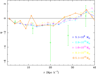
Figure 11: Quadrupole moments of the mean flux from the G6 simulation and SDSS data (stars with error bars). No redshift error has been added.

6 Summary and Discussion

6.1 Summary

In this paper, we have explored the profile of Ly$\alpha$  absorption with distance around quasars using pairs of close-by quasars in high resolution hydrodynamic simulations. We have found the following:

• The mean Ly$\alpha$  forest transmitted flux from a background quasar passing through a region close to a foreground quasar and the infall velocity of matter around a quasar are both dependent on quasar mass.

• We can fit the observed flux vs quasar-pixel separation $r$ to an equation $\exp(-\tau_{\rm eff}(1+(\frac{r}{r_{0}})^{-\gamma}))$ by varying $r_{0}$ and $\gamma$. This simple power law form, derived from fits to the galaxy autocorrelation function works very well.

• There is a strong dependence of $r_{0}$ in this fit to the mass of the quasar host halo in the simulation. From this $r_{0}$ vs. mass relation, we can estimate quasar halo mass.

• The estimated mass of SDSS quasars at $z=3$ is $\log{\rm M/{\rm M_{\odot}}}$=$12.48^{+0.53}_{-0.89}$. We do not see any significant changes in the result when we include redshift errors of  150${\rm\;km\;s^{-1}}$ or a different amplitude of mass fluctuations.

• The estimated halo mass of Lyman Break Galaxies can be found using the same technique. Fitting to the data of Adelberger (2003) we find $\log{\rm M/{\rm M_{\odot}}}=11.13^{+0.39}_{-0.55}$.

• The squashing of flux in redshift space can be quantified using the quadrupole to monopole ratio. There is a no measureable dependence of the squashing effect on halo mass, although the anisotropy seen is consistent with observational data.

6.2 Discussion

Due to their great distance from us, it is difficult to measure the dark matter halo masses of high redshift quasars. For example, few background galaxies exist to make lensing measurements possible, and the rotation curves of their host galaxies may require larger telescopes than currently available to capture.

The strong level of Ly$\alpha$  forest absorption around bright $z=3$ SDSS quasars that we have seen indictates that they have halo masses $\sim 3\times 10^{12}{\rm M_{\odot}}$, comparable to elliptical galaxies at the present. This is not unreasonable because these bright quasars are much rarer than present day ellipticals with this mass. Our mass estimate is roughly 20 times larger than that for the dark matter mass of LBGs at the same redshift, indicating that it is unlikely that bright quasars randomly sample the population of LBGs as hosts.

In our analysis, we have ignored the transverse proximity effect, the possiblity that foreground quasars will decrease the amount of Ly$\alpha$  absorption with local photoionization from their radiation. If this effect is present, it is certainly not dominant, as we have seen that instead there is more absorption close to foreground quasars. If it does exist, but is subdominant, then the true amount of absorption without this extra radiation should be greater and we are underestimating it and hence the halo masses. $\sim 3\times 10^{12}{\rm M_{\odot}}$ therefore represents a lower limit to the dark matter mass of quasar hosts. There are however several ways, including quasar beaming and short lifetimes mentioned in §1 that the transverse proximity effect might not be relevant in any case.

The redshift distortion of the absorption is unfortunately not promising as a complimentary method for constraining the dark matter halo mass. However the insensitity of the distortion to mass means that the correlation function it could be a useful probe of cosmic geometry. As the Ly$\alpha$  forest- quasar clustering signal appears to be much stronger Ly$\alpha$  forest two point clustering, this may be an efficient way of carrying out a high-z Alcock Paczyński test.

References

- (1) Abazajian, K., et al. 2005, Astron. J., 129, 1755
- (2) Adelberger, K. L., Steidel, C. C., Shapley, A. E., Pettini, M., 2003, ApJ, 584, 45
- (3) Adelberger K.L., Steidel C.C., Pettini M., Shapley A.E., Reddy N.A., Erb D.K., 2005, ApJ, 619, 697
- (4) Alcock C., Paczyński B., 1979, Nat, 281, 358
- (5) Bajtlik S., Duncan R. C., Ostriker J. P., 1988, ApJ, 327, 570
- (6) Bruscoli, M., Ferrara, A., Marri, S., Schneider, R., Maselli, A., Rollinde, E., Aracil, B., 2003, MNRAS, 343L, 41
- (7) Cen, R., Miralda-Escudé, J., Ostriker, J. P., & Rauch, M. 1994, ApJ, 437, L9
- (8) Croft, R. A. C., Weinberg, D. H., Katz, N., Hernquist, L., 1998, ApJ, 495, 44
- Croft (2004) Croft, R. A. C., 2004, ApJ, 610, 642
- (10) Croom, S. M., et al. , 2005, MNRAS, 356, 415
- (11) Davé, R., Hernquist, L., Katz, N., Weinberg, D. H., 1999, ApJ, 511, 521
- (12) Hawkins E. et al., 2003, MNRAS, 346, 78
- (13) Hamilton A.J.S., 1992, ApJ, 385, L5
- (14) Hennawi J.F., Prochaska J.X., 2006, submitted to ApJ (/astro-ph/0606084)
- (15) Hernquist, L., Katz, N., Weinberg, D. & Miralda-Escudé, J., 1996, ApJ, 457, L51
- (16) Huchra J.P., Geller M.J., 1982, ApJ, 257, 423
- (17) Jenkins, A., Frenk, C. S., White, S. D. M., Colberg, J. M., Cole, S., Evrard, A. E., Couchman, H. M. P., Yoshida, N, 2001, MNRAS, 321, 372
- (18) Kaiser N, 1987, MNRAS, 1987, 227, 1
- (19) Katz, N., Weinberg, D. H., Hernquist, L., Miralda-Escudé, J., 1996, ApJ, 457, 57
- (20) Mandelbaum, R., Seljak, U., Kauffmann, G., Hirata, C. M., Brinkmann, J., 2006, MNRAS, 368, 715
- (21) McDonald, P, Miralda-Escudé, J., Rauch, M, Sargent, W. L. W., Barlow, T. A., Cen, R., Ostriker, J. P., 2000, ApJ, 543, 1
- (22) Myers, A. D., Brunner, R.J., Nichol, R. C., Richards, G. T., Schneider, D. P., Bahcall, N. A., 2006, ApJ, in press (/astro-ph/0606084)
- (23) Nagamine, K., Cen, R., Hernquist, L., Ostriker, J., Springel, V., 2005, ApJ, 627, 608
- (24) Petitjean, P., Müeket, J.P., Kates, R.E., A&A, 295, 9
- (25) Rauch, M., Miralda-Escudé, J., Sargent, W. L. W., Barlow, T. A., Weinberg, D. H., Hernquist, L., Katz, N., Cen, R., Ostriker, J. P., 1997, ApJ, 489, 7
- (26) Rauch, M, 1998, ARA&A, 36, 267
- (27) Regos, E., Geller, M. J., 1989, AJ, 98, 755R
- (28) Rollinde, E., Srianand, R., Theuns, T., Petitjean, P., & Chand, H., 2005 MNRAS, 361, 1015
- (29) Schaye, J., Aguirre, A., Kim, T.-S., Theuns, T,, Rauch, M, Sargent, W. L. W., 2003, ApJ, 596, 768
- (30) Schirber, M., Miralda-Escudé, J., McDonald, P., 2004, ApJ, 610, 1
- (31) Scott, J., Bechtold, J., Dobrzycki, A., Kulkarni, V. P., 2000, ApJS, 130, 67S
- (32) Seljak, U. et al, 2005, PRD, 71, 103515
- (33) Somerville R.S., Primack J.R., Faber S.M., 2001, MNRAS, 320, 504
- spergel (03) Spergel, D. N., Verde, L., Peiris, H. V., Komatsu, E., Nolta, M. R., Bennett, C. L., Halpern, M., Hinshaw, G., Jarosik, N., Kogut, A., Limon, M., Meyer, S. S., Page, L., Tucker, G. S., Weiland, J. L., Wollack, E.& Wright, E. L., 2003, ApJSupp., 148, 175
- (35) Spergel, D. N. , Bean, R. , Doré, O., Nolta, M. R., Bennett, C. L., Hinshaw, G., Jarosik, N., Komatsu, E., Page, L., Peiris, H. V., Verde, L., Barnes, C., Halpern, M., Hill, R. S., Kogut, A., Limon, M., Meyer, S. S., Odegard, N., Tucker, G. S., Weiland, J. L., Wollack, E., Wright, E. L., submitted to ApJ, (astro-ph/0603449)
- (36) Springel, V., 2005, MNRAS, 364, 1105
- (37) Springel, V. & Hernquist, L, 2003, MNRAS, 339, 289
- (38) Springel, V., Yoshida, N., & White, S.D.M., 2001, New Astronomy, 6, 79
- (39) Theuns, T., Leonard, A., Efstathiou, G., Pearce, F. R., Thomas, P. A., 1998, MNRAS, 301, 478
- (40) Wadsley, J. W., Bond, J. R., 1997, ASPC, 123, 332W
- (41) Weatherley, S.J., Warren, S.J., 2005, MNRAS, 363, 6
- (42) Wyithe, J.S.B, Padmanabhan T., 2006, MNRAS, 366, 1029
- (43) Zehavi I. et al. , 2002, ApJ, 571, 172
- (44) Zhang, Y., Anninos, P., Norman, M.L., 1995, ApJ, 453, 57