Hubble Space Telescope ACS mosaic
of the prototypical starburst galaxy M82

Abstract

In March 2006, the Hubble Heritage Team obtained a large 4-filter (B, V, I, and H$\alpha$) 6-point mosaic dataset of the prototypical starburst galaxy NGC 3034 (M 82 (catalog )), with the Advanced Camera for Surveys (ACS) onboard the Hubble Space Telescope (HST). The resulting color composite Heritage image was released in April 2006, to celebrate Hubble’s 16th anniversary.

Cycle 15 HST proposers were encouraged to submit General Observer and Archival Research proposals to complement and/or analyze this unique dataset. Since our M 82 (catalog ) mosaics represent a significant investment of expert processing beyond the standard archival products, we will also release our drizzle-combined FITS data as a High-Level Science Product via the Multimission Archive at STScI (MAST) in December 2006.

This paper documents the key aspects of the observing program and image processing: calibration, image registration and combination (drizzling), and the rejection of cosmic rays and detector artifacts. Our processed FITS mosaics and related information can be downloaded from:

http://archive.stsci.edu/prepds/m82/

1 Introduction

Last year, the Hubble and Spitzer space telescopes made complementary optical and infrared mosaics, respectively, of The Whirlpool Galaxy M51, see Mutchler et al. (2005); Calzetti et al. (2005). This year, the starburst galaxy M82 received similar treatment, described by this paper and Engelbracht, et al. (2006), respectively. Although we released the color composite image of the Hubble M82 mosaic in April 2006 (see press release URL below), the science data are embargoed until December 2006.

M82 (catalog ) hosts the nearest (D=3.6 Mpc) example of a giant starburst galaxy, with many key processes, such as super star clusters, ISM interfaces, and outflows, occurring on scales that benefit from Hubble’s high angular resolution for their study.

2 Observations

Our observing program (HST proposal 10776) produced 96 individual exposures with the ACS Wide Field Channel (WFC). The WFC is composed of two 4096x2048 pixel CCD arrays butted together, with a small gap (equivalent to 50 pixels wide) between them. The total WFC field-of view is about 200 square arcseconds. For each of the four filters (Johnson B,V,I, and H$\alpha$), four exposures were obtained at six slightly overlapping pointings or “tiles” in a 3x2 mosaic, at a telescope orientation of 130 degrees. The exposure times for each filter are summarized in Table 1.

The four exposures within each tile were dithered. A small sub-pixel dither (2.5 x 1.5 pixels) improves the rejection of detector artifacts as well as cosmic rays, coupled with a larger dither which spans the interchip gap (5x60 pixels), so the combined mosaic will not have strips of missing data there. These patterns are fully described on the ACS dither webpage:

http://www.stsci.edu/hst/acs/proposing/dither/

3 Pipeline data calibrations

The standard archival data was retrieved and automatically calibrated on-the-fly via the Multimission Archive at STScI (MAST), after the best calibration reference files became available (a few weeks after the observations). This standard ACS pipeline (CALACS) processing includes bias, dark, and flat-field corrections. The calibration reference files also propagate data quality flags which identify many types of detector artifacts, most of which were excluded during the MultiDrizzle processing described below. These include bad CCD columns, hot pixels (and their CTE tails), warm pixels, and saturated pixels. For further details of standard calibrations are provided in the ACS Data Handbook, Pavlovsky et al. (2005). The latest calibration reference files, and definitions of data quality flags are available on the ACS website:

http://www.stsci.edu/hst/acs/analysis/reference_files

As input to the drizzle-combination described below, we used the archival flat-fielded images (_flt.fits or hereafter simply flt). Since this dataset is not associated, the pipeline currently generates single-image drizzled output (_drz.fits) for each exposure. Although MultiDrizzle was added to the ACS pipeline in 2004, the HST ground system can only combine associated datasets, and in any case, cannot assemble large mosaics. In the standalone environment, however, MultiDrizzle can be used to combine any set of images, generating it’s own association table (_asn.fits) for all the input exposures. Note that this table also gets updated with the shifts and rotations provided in the shiftfile, to register the mosaic (as described below).

4 Image registration

Our image combination software uses the World Coordinate System (WCS) information in the image headers to align the images. This works very well for data taken within the same visit, or otherwise utilizing the same guide stars. Such data are typically aligned to within at least 0.2 WFC pixels (0.01 arcsec). But mosaic datasets involving shifts larger than about 100 arcseconds necessarily involve different guide stars in different visits, and so guide star positional errors render the WCS unreliable for adequate image registration.

We use stars in the images to register the frames, and since more stars are detected in the I-band (F814W), we use those images to measure relative positions and derive delta-shifts (relative to the WCS). We arbitrarily define the first POS2 (visit 21) I-band frame (rootname j9l021d5q) to be the origin of our reference frame (0,0,0). Since the POS2 exposures for each filter executed in the same visit, they are well-aligned to each other. Therefore, the filter-to-filter registration is adequate, and we can apply the I-band shifts to the other filters with confidence. After the I-band shifts were applied to the other filters, their alignment was spot-checked, and individual stars across all four filters were verified to be well-registered.

We use tweakshifts for the final refinement of the shifts. But tweakshifts only works within the regime where the images to be registered are already aligned to within about 1 pixel, and with little or no rotation involved. So the large shifts between the tiles must be removed before we can run tweakshifts.

4.1 Intertile shifts

The data for each tile were obtained in different visits, so the tiles can therefore be misaligned on the order of 10 pixels, and rotated with respect to each other due to the nominal roll of the spacecraft. Fewer stars are available to measure these “intertile” shifts, since they must lie in the narrow tile overlaps.

These initial intertile shifts were measured using only the first of the four frames within each tile. MultiDrizzle was run only through the driz_separate step, to generate the single-drizzled (distortion corrected _single_sci.fits) versions of these images in the undistorted mosaic output space. We set clean=no to save the _single_sci.fits files, and avoid altering the input flt images by setting skysub=no (no sky subtraction). Suitable registration objects (preferably stars, but sometimes clusters with a sharp peak) were visually selected: they must appear in multiple frames, be free of obvious cosmic ray contamination, and not be saturated and bleeding. With imexam, the x,y positions of 10-20 objects were measured in the tile overlap regions. The POS1, POS3, and POS5 tiles have long overlaps with the POS2 reference tile, so objects were chosen which span the full length of each overlap. The POS1 and POS6 tiles have very small overlaps with POS2, so their shifts were measured iteratively, i.e. after the corrective shifts and rotations had been applied to POS1, POS3, and POS5. Then stars in their much larger overlaps with POS1 and POS6 could also be used to measure shifts, with greater leverage.

The measured star positions were used as input to the geomap task, which can solve for shifts and rotations. The corrections for the six primary intertile frames were also applied to the other three frames in their respective tiles, thereby internally registering the entire mosaic. The shifts and rotations were assembled into a shiftfile, to be provided as input to MultiDrizzle.

4.2 Intratile shifts

To generate the files needed for refining the shift measurement with tweakshifts, MultiDrizzle was again run only through the driz_separate step, applying the intertile delta-shifts derived above. Then tweakshifts was run for overlapping sets of I-band _single_sci.fits images, this time using all the images in each tile (not just the first frame), such that the refinement includes any small “intratile” shifts. With a tolerance of 0.7 pixels and a 6 sigma threshold, tweakshifts typically detected on the order of 10,000 objects (most of which are cosmic rays and other artifacts) and matched a few percent of those objects within each tile. The rotations measured initially (as a check) were insignificant, so we solved only for x,y shifts. These intratile refinements were then summed with the initial intertile shifts, to create the shiftfiles provided to MultiDrizzle for the final image combinations.

5 Masking artifacts

In addition to the detector artifacts automatically flagged by the calibration pipeline, we can manually mask observational artifacts that we’d similarly like to exclude from our data, and which are too diffuse or large to get rejected along with the cosmic rays. The variety of artifacts which might be seen are described on the ACS anomalies webpage:

http://www.stsci.edu/hst/acs/performance/anomalies

First, we note two significant artifacts which we do not attempt to mask or correct. This dataset was afflicted by some filter reflections (or “optical ghosts”) from several bright foreground stars, which appear as figure-8 or doughnut features (see Figure 1). But since the ghosts overlap each other, leaving no good data in any of the frames being combined, we chose not to mask them. Some amplifier crosstalk is also evident in the mosaics, H$\alpha$ POS3 in particular, where both the bright star and galaxy create negative mirror-image imprints in the opposite amplifier quadrant. This effect is not significant, and we do not attempt to mask or correct it.

Some satellite trails were masked and excluded as follows. The endpoints and width of each satellite trail were measured in the undistorted _single_sci.fits images. Then the satmask task (Richard Hook, private communication) was used to generate a mask for each trail. This undistorted mask was then transformed (using blot) into the input distorted space of the flt images, assigned the unique flag value of 16384, and summed with the existing flt data quality array, e.g.j9l051gnq_flt.fits[DQ,1]. Any such masking creates even more areas of reduced signal-to-noise, and the affected areas are reflected in the weight maps.

6 Image combination

The IRAF/STSDAS MultiDrizzle task (Koekemoer et al., 2002) was used to combine the mosaics for each filter. MultiDrizzle is a PyRAF script which performs, on a list of input flt images: bad pixel identification, sky subtraction, rejection of cosmic rays and other artifacts (as described above), and a final drizzle combination (Fruchter et al., 2002) with the cosmic ray masks, into a clean image. MultiDrizzle also applies the latest filter-specific geometric distortion corrections to each image, as specified in the IDCTAB reference tables. These mosaics were processed in the same environment as the HST calibration pipeline (SunFire/smalls). See:

http://www.stsci.edu/hst/acs/analysis/multidrizzle/

Although the rejection of cosmic rays and other undesireable artifacts is embedded in the MultiDrizzle processing, the following is an overview of how it is accomplished. A median image is constructed from the registered and undistorted single-drizzled (_single_sci.fits) images. This median image – or the appropriate sections of it – are blotted back to the distorted space of the input flt images, where it can be used to identify cosmic rays. The dither package tasks of deriv and driz_cr are used to compare this blotted image and its derivative image with the original input flt file, and generate a cosmic ray mask. Finally, all the flt images, together with their newly created cosmic ray masks, are drizzled onto a single output mosaic, which has units of electrons per second in each pixel.

There are many MultiDrizzle parameters which can be adjusted. The pipeline uses carefully pre-defined sets of parameters (defined in the MDRIZTAB table identified in image headers), but in the standalone environment, optimal combination parameters for a specific dataset can be found through some trial-and-error iterations. Here we describe our key parameter settings, especially any non-default choices. The full set of drizzling parameters are available in the README file on the MAST M82 webpage.

We set the center of the output mosaic to be the coordinates for M82 given by the NASA Extragalactic Database (in decimal degrees ra = 148.967580, dec = 69.679704), and rotate the output with north up, and east left (final_rot=0.0). We set the output dimensions as 12288x12288 pixels, which truncates a small number of pixels in the corners of the rotated mosaic (Figure 1). We provide a shiftfile to refine the mosaic registration as described in the previous section. Since the galaxy fills most of the mosaic, sky subtraction was turned off (skysub=no). We set crbit=0 so that our rejections do not get flagged in the data quality arrays of the input flt images. Note that the weight maps reflect the cosmic rays and artifacts rejected by MultiDrizzle. The cosmic ray rejection thresholds (driz_cr_snr = 4.0 3.5) were raised a bit to avoid rejecting the cores of bright objects. Since these mosaics are so large, we did not build them into multi-extension FITS files (build=no), i.e. the science array and weight maps are separate files, and we chose not to produce context images. Wet set bits=4192 to ignore the flags for the warm pixels (flag=32) and CTE tails of hot pixels (flag=64), which are flagged in the dark reference image, and any rejections flagged by pipeline processing (flag=4096). We use the default square drizzle kernel (final_kernel=square), which performs well in most cases. Some correlated noise is evident as a faint Moire-like pattern in the weight maps, which is also visible in the science data – especially in low signal-to-noise areas. Although the lanczos3 and gaussian kernels can suppress this correlated noise better, they may also enhance unrejected artifacts.

The cosmic ray masks generated by MultiDrizzle are used as input to the final drizzle combination of all the images. The drizzle task (Fruchter and Hook, 2002) performs a weighted sum of the input images, and allows input pixels to be shrunk (we set pixfrac=0.9) before being mapped onto the output plane. The output pixel scale (final_scale) can also be different than the input (detector) pixel scale – a smaller pixel scale can allow more spatial information to be recovered if the data are well-dithered. Since our 2-point sub-pixel dither pattern does not sample optimally in both dimensions, even in conjuntion with the gap dither, we retain the input WFC pixel scale (0.05 arcsec/pixel), rather than drizzle to a finer output scale.

MultiDrizzle also produces exposure weight maps, which indicate the background and instrumental noise for each pixel in the science data. In general, we acheived a relatively uniform exposure weight across the entire mosaic. But the total exposure time can vary significantly from pixel-to-pixel, mainly due to overlaps between adjacent tiles, interchip gaps, and all the bad pixels which are rejected. The weight maps were visually inspected to ensure that rejected artifacts have appropriately lower weight – and equally importantly, that real objects (e.g. the cores of stars, or of the core of M82) were not rejected. The only irregular rejection was related to long diffraction spikes and/or bleeding (from saturation) around bright foreground stars, which is to be expected. Small amounts of residual artifacts or cosmic ray contamination may have survived rejection – most likely in areas of low weight, such as the gap overlaps.

The photometric fidelity of the MultiDrizzle code is reliable to a high degree of accuracy, since the underlying algorithm for drizzle is designed to be flux-conserving (see Fruchter & Hook, 2002, and Koekemoer et al., 2002). The MultiDrizzle team has verified this in practice by using a suite of test datasets to compare photometry from different exposures of the same objects, and verifying that these provide good agreement to better than the ACS flatfield and photometric calibration accuracy (1-2%) for bright sources, and Poisson noise for fainter sources. But these M82 mosaics were not tested for photometric accuracy, and were only spot-checked for PSF stability across the field.

7 Data products and filenaming convention

The drizzled mosaics described in this paper are available as High-Level Science Products (HLSP) via the Multimission Archive at STScI (MAST):

http://archive.stsci.edu/prepds/m82/

The filenames of our drizzled science mosaics (_drz_sci.fits) and their corresponding exposure weight maps (_drz_weight.fits), are listed in Table 1. This filenaming convention allows these HLSP files to be queryable via MAST archive searches. The filenames indicate the filter (b,v,i,h), and the pixel scale of 0.05 arcsec (s05). These files have dimensions of 12288 x 12288 pixels (10.24 x 10.24 arcminutes) and are 604 MB each (uncompressed). Lower resolution (1/4) block-averaged FITS versions of each mosaic were also produced using the IRAF blkavg task, mainly for quick-look downloading and viewing, or for educational purposes (not intended for scientific analysis). These have a scale of 0.20 arcsec per pixel (s20 in the filenames), dimensions of 3072 x 3072 pixels, and are 38 MB each, or 1/16 the filesize of the full-resolution mosaics above. Much smaller preview GIF images of these mosaics are also available on the MAST website. Note that the FITS data are all oriented with north up, and east to the left (as in Figure 1), whereas the press release color composite image (Figure 3) is at a position angle of 130 degrees. The color composite image and related information are available from the associated STScI and Hubble Heritage press releases:

http://hubblesite.org/newscenter/newsdesk/archive/releases/2006/14/

http://heritage.stsci.edu/2006/14/

8 Acknowledgments

Thanks to STScI Director Matt Mountain for granting 24 orbits of Director’s Discretionary observing time to the Hubble Heritage Team to conduct this program. Thanks also to Warren Hack, Chris Hanley, Richard Hook, Marco Sirianni, Anton Koekemoer, Inga Kamp, Karen Levay, Faith Abney, and Randy Thompson for their contributions to this project.

If you utilize these prepared mosaics for further scientific analysis, please acknowledge and/or reference this paper.

Table 1: Filters, total exposure times, and mosaic filenames.

Filter	Exposure Time	Science Mosaic	Weight Map
F435W (B)	1600s	h_m82_b_s05_drz_sci.fits	h_m82_b_s05_drz_weight.fits
F555W (V)	1360s	h_m82_v_s05_drz_sci.fits	h_m82_v_s05_drz_weight.fits
F814W (I)	1360s	h_m82_i_s05_drz_sci.fits	h_m82_i_s05_drz_weight.fits
F658N (H$\alpha$)	3320s	h_m82_h_s05_drz_sci.fits	h_m82_h_s05_drz_weight.fits

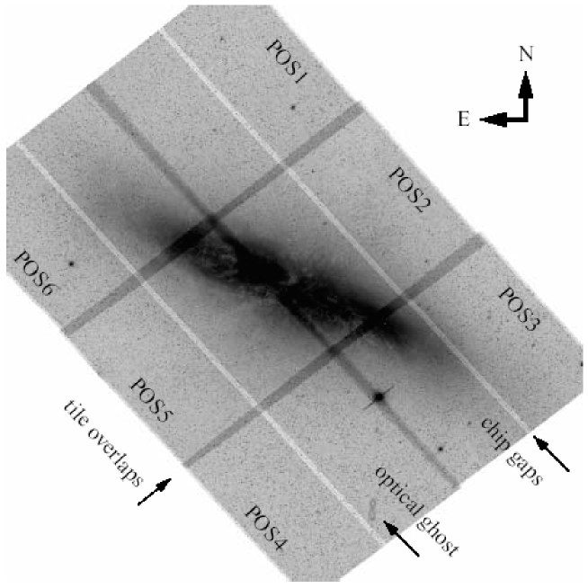
Figure 1: Raw B-band (F435W) mosaic (intertiles only) illustrating the orientation and some key features of the 3x2 mosaic data. The mosaic files have dimensions of 12288 x 12288 pixels (10.24 x 10.24 arcminutes). With north up and east to the left, the data is truncated slightly in each corner.

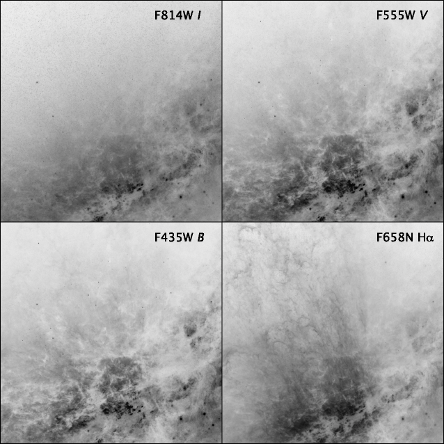
Figure 2: Close-up of M82 galactic features in all four filters. North is not up here.

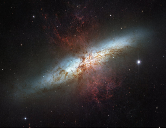
Figure 3: Color composite mosaic of M82 made from all four filters. Note this press release image is at a position angle of 130 degrees (north is not up here).

References

- Calzetti et al. (2005) Calzetti, D., et al., ApJ, 633, 871-893
- Engelbracht, et al. (2006) Engelbracht, C. W., et al., ApJ, 642, 127-132
- Fruchter et al. (2002) Fruchter, A., & Hook, R., 2002, PASP, 114, 144
- Koekemoer et al. (2002) Koekemoer. A. et al., 2002, HST Calibration Workshop, Ed. S. Arribas, A. M. Koekemoer, B. Whitmore (STScI: Baltimore), p.337
- Mutchler et al. (2005) Mutchler, M., et al., 2005, BAAS, 37, 2
- Pavlovsky et al. (2005) Pavlovsky, C., et al., 2005, ACS Data Handbook, version 4.0