Microlensing of an extended source by a power-law mass distribution

Abstract

Microlensing promises to be a powerful tool for studying distant galaxies and quasars. As the data and models improve, there are systematic effects that need to be explored. Quasar continuum and broad-line regions may respond differently to microlensing due to their different sizes; to understand this effect, we study microlensing of finite sources by a mass function of stars. We find that microlensing is insensitive to the slope of the mass function but does depend on the mass range. For negative parity images, diluting the stellar population with dark matter increases the magnification dispersion for small sources and decreases it for large sources. This implies that the quasar continuum and broad-line regions may experience very different microlensing in negative-parity lensed images. We confirm earlier conclusions that the surface brightness profile and geometry of the source have little effect on microlensing. Finally, we consider non-circular sources. We show that elliptical sources that are aligned with the direction of shear have larger magnification dispersions than sources with perpendicular alignment, an effect that becomes more prominent as the ellipticity increases. Elongated sources can lead to more rapid variability than circular sources, which raises the prospect of using microlensing to probe source shape.

1 Introduction

Microlensing is an increasingly important tool for studying small-scale structure in lens galaxies and source quasars. In recent years, microlensing has been observed in a number of multiply-lensed quasars (e.g., Woźniak et al., 2000; Schechter et al., 2003; Richards et al., 2004; Keeton et al., 2006; Paraficz et al., 2006). Microlensing modeling has also been improving. For example, Kochanek (2004) has introduced a sophisticated technique for analyzing light curves. Even so, there are aspects of the models for the lens and source that still need to be considered for microlensing to reach its full potential. This is especially important for quasar microlensing, where several length scales are involved.

Different regions of a quasar emit radiation in roughly distinct bands. For example, continuum (blackbody) radiation in the optical and x-ray bands is emitted from the accretion disk surrounding the supermassive black hole, while broad emission lines in the optical and UV are thought to originate from clouds in a region outside of and larger than the accretion disk. Radio emission comes from even larger structures. Roughly speaking, a source can only be affected by objects in the lens galaxy whose Einstein radii are comparable to or larger than the source size. Consequently, the continuum, broad-line, and radio regions probe different structures in the lens galaxy. Radio jets can be used to probe dark matter substructure (Metcalf & Madau, 2001; Dalal & Kochanek, 2002) in lens galaxies while the accretion disk (Jaroszyński, Wambsganss & Paczyński, 1992; Mortonson, Schechter & Wambsganss, 2005; Pooley et al., 2006) and broad-line region (BLR) are used for studying the stellar component (Schneider & Wambsganss, 1990; Richards et al., 2004; Keeton et al., 2006). In principle, both methods can also be used to examine the light source. This is of particular interest for the BLR whose properties are not well understood (e.g., Peterson & Horne, 2005). In this paper we investigate the potential of microlensing to deepen our knowledge of the BLR and accretion disk and to determine both the abundance and mass function of stars in lens galaxies.

Until recently, sources relevant for microlensing could not be resolved. Therefore, many theoretical models have assumed a point source, and have focused on determining properties of the lensing galaxy. Such investigations have found that microlensing magnification distributions are not very sensitive to the shape of the microlens mass function if it spans an order of magnitude or so in mass (e.g., Wyithe & Turner, 2001). The magnification distributions do look different if there are two distinct mass components: not just stars, but also “dark matter” that could come in the form of a smooth mass component (e.g., Schechter & Wambsganss, 2002), or a set of discrete objects that are much less massive than the stars (Schechter, Wambsganss & Lewis, 2004; Lewis & Gil-Merino, 2006). We generalize the previous studies by considering microlensing of an extended source. The source size $R_{S}$ introduces a new length scale, which heuristically divides the microlenses into two categories: microlenses with $R_{E}\ga R_{S}$ are massive enough to be felt individually, while microlenses with $R_{E}\la R_{S}$ act like a smooth component. We therefore conjecture that the finite source size makes the magnification distributions sensitive to the microlens mass function even when it spans just 1–1.5 orders of magnitude. Lewis & Gil-Merino (2006) recently studied microlensing of an extended source by a bimodal mass function; we now consider a continuous mass function.

Studying microlensing of an extended source is especially relevant for the BLR, because recent observations suggest it has a size $R_{BLR}\sim 10^{16}$–$10^{18}$ cm (Richards et al., 2004; Keeton et al., 2006) comparable to stellar Einstein radii. Understanding the effects of source size should help us probe BLR length scales more precisely. We perhaps should not expect to probe the BLR surface brightness distribution, however; Mortonson, Schechter & Wambsganss (2005) suggest that microlensing is not very sensitive to the source brightness profile. Their assertion is based on simulations of circular sources with several specific surface brightness profiles. We perform similar “numerical experiments” to consider other source properties, notably shape and geometry.

The possibility of a non-circular source has not been considered in previous microlensing analyses. However, accretion disks viewed at random inclinations would generically appear elliptical rather than circular. A similar situation may apply to the BLR if it has a disky structure (e.g., Murray & Chiang, 1998; Elvis, 2000; Richards et al., 2004). We also consider annular accretion disks. Such models are important for two reasons. First, quasar accretion disks have inner radii defined by the innermost stable circular orbit of a particle in motion around the central black hole. Second, typical models (e.g., the Shakura-Sunyaev disk), emit over a wide range of wavelengths, with each band corresponding to different annular regions.

This paper is organized as follows. Lens modeling and simulations are discussed in §2. Our results are presented in §3. We first consider the general problem of how source size and lens mass impact microlensing (§3.1). In following subsections, we investigate the effects of dark matter (§3.2), source profile (§3.3), source ellipticity and position angle (§3.4), and accretion disk geometry (§3.5). We construct light curves in §3.6 to investigate variability timescales. Our conclusions are summarized in §4.

2 Methods

We consider microlensing of an extended source by a distribution of stars and dark matter. We zoom in on a region in the lens galaxy around a lensed image. The size of the region is chosen to satisfy two conditions. First, it must be large compared to a typical stellar Einstein radius, which is the relevant scale for microlensing. Second, it must be small compared to the scale of the lens galaxy, namely the image separation. The latter allows us to take the mean densities of stars and dark matter to be constant. These criteria are not very restrictive since Einstein radii are typically on scales of microarcseconds while image separations are on scales of arcseconds.

We describe the stellar population of the lens by a mass function $dN/dm$, which gives the number of stars per unit mass between $m$ and $m+dm$. We use a power law of the form

$$\frac{dN}{dm}\propto m^{-\alpha}\qquad(m_{1}\leq m\leq m_{2})\,,$$ (1)

for some $m_{1}$ and $m_{2}$. Rather than specifying the mass limits $m_{1}$ and $m_{2}$ explicitly, we adopt the equivalent approach of giving the ratio $m_{1}/m_{2}$ along with the mean mass $\bar{m}$. A typical choice for the power law index is $\alpha=2.35$, the Salpeter initial mass function. The mass function is normalized so that the scaled mass density is $\kappa_{*}$. In addition to stars, the galaxy may include a continuous component with density $\kappa_{c}$. The final ingredient is the shear $\gamma$, which accounts for tidal forces from outside the patch of stars being considered. To obtain a relation between $\kappa$ and $\gamma$ we must choose a mass model for the lens galaxy. We use a singular isothermal ellipsoid for which $\kappa=\gamma$. This model is simple and provides a reasonable fit to observed systems (e.g., Treu & Koopmans, 2004; Rusin & Kochanek, 2005; Treu et al., 2006).

In the absence of microlensing, the magnification is given by

$$\mu_{0}=[(1-\kappa)^{2}-\gamma^{2}]^{-1}\,,$$ (2)

where $\kappa=\kappa_{*}+\kappa_{c}$. We consider a typical bright image with $\mu_{0}=\pm 10$ corresponding to $\kappa=\gamma=0.5\mp 0.05$. In microlensing, the spatial distribution of stars is random, so the magnification at a given time will be drawn from a probability distribution. If the distribution is broad, then chances are high that the magnification will differ from that predicted for a smooth model, viz. $\mu_{0}$. The effects of microlensing are therefore naturally described by the dispersion (standard deviation) of the probability distribution.

Computing the magnification distribution for given $\kappa$, $\gamma$ and $dN/dm$ can only be done numerically. We use the microlensing code of Wambsganss (1999), which gives the magnification of a point source as a function of position over a square region of the source plane with side length $L=15R_{E}(M_{\odot})$. In mean mass units the side length is given by $L=15R_{E}(\bar{m})$ for $m_{1}/m_{2}=1$, $L=31.71R_{E}(\bar{m})$ for $m_{1}/m_{2}=0.1$, and $L=52.26R_{E}(\bar{m})$ for $m_{1}/m_{2}=0.03$. We create magnification maps with a resolution of $L/1024$ (see Figure 1). To obtain a statistical sample, we perform 100 realizations for each set of parameters we consider.

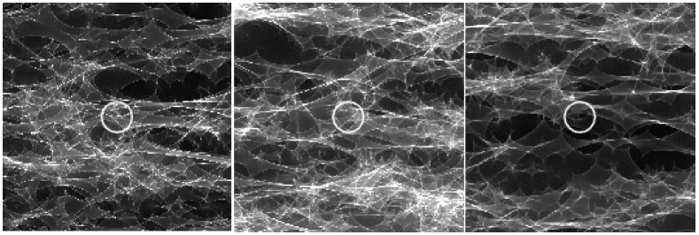
Figure 1: Magnification maps for a positive-parity image with $\kappa=\gamma=0.45$, implying a macro-magnification of $\mu_{0}=10$. The gray scale indicates the magnification with values in the range $\mu=1$ (black) and $\mu=30$ (white). Panels show Salpeter mass functions with $m_{1}/m_{2}=1$ (left), 0.1 (middle), and 0.03 (right). Each map has a side length $L=15R_{E}(\bar{m})$. Magnification histograms are generated by convolving the surface brightness profile of the source (indicated by circles) with the magnification map.

We must convolve the magnification map with a surface brightness profile in order to compute the magnification of an extended source. We use Gaussian, uniform and linear profiles, respectively defined by

$$I_{1}(R)\equiv\frac{\ln 2}{\pi R_{S}^{2}}\exp\left(-\frac{R^{2}\ln 2}{R_{S}^{2}}\right) (0\leq R<\infty),$$ (3)

$$I_{2}(R)\equiv\frac{1}{2\pi R_{S}^{2}} (0\leq R\leq\sqrt{2}R_{S})$$ (4)

and

$$I_{3}(R)\equiv\frac{3}{4\pi R_{S}^{2}}\left(1-\frac{R}{2R_{S}}\right) (0\leq R\leq 2R_{S})\,,$$ (5)

where $R_{S}$ is the half-light radius of the source, and the sources are normalized to unit flux. In microlensing, the natural length scale is the Einstein radius of the mean mass star (e.g., Lewis & Irwin, 1996). We henceforth quote the source size as $r_{S}\equiv R_{S}/R_{E}(\bar{m})$.

These models are simple but nevertheless useful. The Gaussian model is popular in microlensing studies (e.g., Wambganss, Paczyński & Schneider, 1990; Wyithe, Agol & Fluke, 2002), so it is good to include. The uniform disk is the simplest model conceivable, while the linear disk has at least one physical connection. These same three models were used by Mortonson, Schechter & Wambsganss (2005), so we can compare their results with ours. While Mortonson, Schechter & Wambsganss (2005) (and many others) applied the models to accretion disks, we imagine that they are useful for describing BLRs as well. In particular, the linear disk is similar to the biconical BLR of Abajas et al. (2002).

We consider an elliptical source by making the substitution

$$I(R)\rightarrow I(\rho)/q,$$ (6)

with minor-to-major axis ratio $q$ and elliptical radius defined by $\rho^{2}\equiv R^{2}\cos^{2}\theta+R^{2}\sin^{2}\theta/q^{2}$. We also consider a uniform annular disk, with inner-to-outer radius ratio $Q$, by making the replacement

$$I_{2}(R)\rightarrow I_{2}(R)\frac{1+Q^{2}}{1-Q^{2}},$$ (7)

for radii satisfying

$$\frac{\sqrt{2}QR_{S}}{1+Q^{2}}\leq R\leq\frac{\sqrt{2}R_{S}}{1+Q^{2}}.$$ (8)

In the following section our fiducial model assumes a Gaussian source and a lens described by a stellar population whose masses are given by a Salpeter mass function with $m_{1}/m_{2}=0.1$. We assume that $\kappa=\kappa_{*}=0.5\mp 0.05$ for images of positive and negative parity, respectively. We explicitly state when other models are to be used.

3 Results

Figure 2: Mass functions with fixed means, $\bar{m}$, for various mass ranges, $m_{1}/m_{2}$, and logarithmic slopes, $\alpha$. The top panel shows mass functions with $\alpha=2.35$. The solid, dotted and dashed curves have $m_{1}/m_{2}$= 1, 0.1, and 0.03, respectively. The bottom panel shows mass functions with $m_{1}/m_{2}=0.1$. The solid, dotted and dashed curves show $\alpha$= 1.85, 2.35 and 2.85, respectively.

Figure 3: Magnification histograms for different source sizes and mass functions for a positive-parity image with $\left|\mu_{0}\right|=10$. Columns show source sizes in mean-mass Einstein radii of $r_{S}=$0.1, 0.4, 0.7 and 1.0. The top row shows mass functions with logarithmic slopes of $\alpha=2.35$. The solid, dotted, and dashed curves have $m_{1}/m_{2}$=1, 0.1 and 0.03, respectively (see Figure 2, top panel). The bottom row shows mass functions with $m_{1}/m_{2}$=0.1. The solid, dotted, and dashed curves have $\alpha=$1.85, 2.35 and 2.85, respectively (see Figure 2, bottom panel).

We now study microlensing of an extended source by a power-law mass distribution. Wyithe & Turner (2001) conclude that point-source microlensing magnification distributions are not significantly affected by the choice of mass function. We consider whether this result can be extended to the case of a finite source (§3.1). Dark matter can affect microlensing in surprising ways, raising the possibility of using microlensing to measure the density of dark matter at the image positions (Schechter & Wambsganss, 2002, 2004). We generalize earlier work by including a mass function of stars and an extended source (§3.2).

We also explore how varying properties of the source impacts microlensing magnification distributions. In §3.3, we describe a source by three surface brightness profiles. We broaden the discussion in §3.4 to include elliptical sources. Finally, we consider annular sources in §3.5.

3.1 Source Size and Lens Mass

We begin by examining how microlensing of a finite source is affected when we vary the mass range and logarithmic slope of the mass function (cf. Wambsganss, 1992). Figure 2 shows the mass functions we use. Figures 3 and 4 show magnification histograms for the different mass functions and different source sizes, for positive and negative parity. First consider the effects of the mass range, shown in the top row of each figure. Increasing the mass range causes the magnification distribution to broaden slightly, especially for larger sources. This is shown more directly in the top panel of Figure 5, which plots the magnification dispersion versus source size for the different mass ranges (for the positive parity case). When the source is small we recover the previous result that the mass range does not affect the magnification distribution (Wyithe & Turner, 2001). However, as the source gets larger there is more difference between the three mass functions.

Figure 4: Similar to Figure 3, but for a negative parity image with $\left|\mu_{0}\right|=10$.

Figure 5: Dispersion in log $|\mu|$ computed from histograms for source sizes in the range $0\leq r_{S}\leq 4$ (see, e.g., Fig. 3) versus source size for different mass functions, for a positive-parity image with $\left|\mu_{0}\right|=10$. The top panel shows mass functions with logarithmic slopes of $\alpha=2.35$. The solid, dotted, and dashed curves have $m_{1}/m_{2}$ = 1, 0.1 and 0.03, respectively. The bottom panel shows mass functions with $m_{1}/m_{2}=0.1$. The solid, dotted, and dashed curves have $\alpha$ = 1.85, 2.35 and 2.85, respectively.

To understand why the magnification dispersion increases as the mass range increases, we return to Figure 2. The top panel shows that increasing the mass range causes the mass function to “spread out”: the lower limit decreases slightly, while the upper limit can increase substantially. A high upper limit allows massive stars to exist, although they will be fairly rare because the mass function is steep. Thus, some magnification maps will contain one or a few massive stars that significantly affect the microlensing, while many will not. We believe this explains why increasing the mass range increases the magnification dispersion. It also explains why the mass range becomes more important as the source size increases: large sources are most sensitive to massive stars.

Now consider the slope of the mass function. Figures 3–5 show that the slope hardly affects microlensing at all, regardless of the source size. The reason is that changing the slope shifts the mass function left or right (see Figure 2), but not dramatically.

We conclude that microlensing of an extended source may offer the possibility of determining the dynamic range ($m_{1}/m_{2}$) of the stellar mass function, but not for determining the mass function slope. In light of this result, we henceforth restrict our attention to a Salpeter mass function ($\alpha=2.35$), and we focus attention on the case $m_{1}/m_{2}=0.1$.

3.2 Dark Matter Content

Figure 6: Magnification histograms for an image with $|\mu_{0}|=10$ for different dark matter mass fractions. From top to bottom, panels show $f_{\rm c}$ = 0.2, 0.4, 0.6, 0.8, and 0.99. The left and right columns have $r_{S}$ = 0.1, and 0.5, respectively. The solid and dotted curves have positive and negative parity, respectively. We use a Salpeter mass function ($\alpha=2.35$) with $m_{1}/m_{2}=0.1$.

Figure 7: Dispersion in log $|\mu|$ computed from histograms for source sizes in the range $0\leq r_{S}\leq 5$ (see, e.g., Fig. 6) versus source size for different dark matter fractions. The top (bottom) panel shows an image with positive (negative) parity. The solid, dotted, dashed, dot-dashed and dot-dot-dashed curves have $f_{\rm c}$ = 0.2, 0.4, 0.6, 0.8, and 0.99, respectively.

We now consider how the mass fraction in dark matter affects microlensing. Controversy remains as to whether cosmological simulations of dark matter agree with galaxy observations (e.g., Spekkens, Giovanelli & Haynes, 2005; Gerhard, 2006, and references therein). Part of the problem is that most observations (galaxy dynamics, gravitational macrolensing) depend on the global mass distribution in a galaxy, rather than the local mass density. Schechter & Wambsganss (2002, 2004) argue that microlensing offers a new way to measure the density of dark matter at the positions of the lensed images. They consider a uniform mass function and a point source; we generalize the analysis to a mass function and an extended source.

Figure 6 shows magnification histograms for dark matter mass fractions of $f_{c}\equiv\kappa_{c}/\kappa$ = 0.2, 0.4, 0.6, 0.8, and 0.99. One might expect that as $\kappa_{c}$ is increased, microlensing would become less important, since fewer stars produce simpler caustic networks. For $\kappa_{c}\rightarrow\kappa$ the magnification distribution indeed approaches a $\delta$-function centered at $\mu_{0}$, as seen in the bottom row of Figure 6.

For smaller values of $\kappa_{c}$, however, the histograms show more structure. In particular, secondary peaks appear in several of the histograms (see, e.g., Rauch et al., 1992). The different peaks correspond to different numbers of microimages (see Granot, Schechter & Wambsganss, 2003, especially Figure 4). If dark matter is the primary mass component, the probability that a source will have multiple microimages is low. In that case, the magnification distribution has a single peak near the expected magnification in the absence of microlensing (e.g., $f_{c}=0.99$). For smaller values of $f_{c}$, the density of caustics increases, which in turn raises the probability that a source will have extra microimage pairs. The magnification distribution therefore acquires a second peak associated with regions of the source plane for which an extra image pair is created (see left-hand column of Figure 6). When $f_{c}$ is low, regions with extra microimages become the norm, and the peaks corresponding to different numbers of microimages become less distinct. Also, an extended source often covers regions with different numbers of microimages, smearing out the effects of additional microimages (see right-hand column of Figure 6).

Figure 6 also demonstrates the importance of parity. We find that negative parity images lead to distributions with tails at low magnification. Schechter & Wambsganss (2002) find the same behaviour for a point source. As the source size is increased, the tails become less apparent. When $r_{S}=1.0$ (not shown), the two parities give nearly identical results. One surprise is that a difference between positive and negative parity can be observed in the skewness of the distributions even for $f_{c}=0.99$. This means that even a small stellar mass fraction gives rise to noticeable parity-dependent effects.

Figure 7 uses the magnification dispersion to quantify the effects of parity and source size. In the positive parity case (top panel), replacing stars with dark matter decreases the dispersion for all source sizes, which makes intuitive sense. However, in the negative parity case (bottom panel) when the source is small, diluting the stars with dark matter increases the dispersion, at least in the range $f_{c}\leq 0.8$. Schechter & Wambsganss (2002) first found this result for a point source and a uniform stellar mass function. We now see that it holds for small extended sources as well. We discover though, that when the source is large, the trend reverses: increasing the dark matter fraction decreases the magnification dispersion. It seems notable that the curves of dispersion versus source size for different dark matter fractions all cross at roughly the same source size ($r_{S}\sim 0.8$), although we do not know whether this is significant.

It is worth pointing out that Dobler, Keeton & Wambsganss (2006) examine the effects of dark matter and source size on the magnification for demagnified lensed images. They find that increasing the dark matter fraction always decreases the magnification dispersion for a demagnified negative parity image. (Recall that our negative parity image is magnified.) However, for a demagnified central image, diluting the stars with dark matter increases the dispersion for a small source, but decreases the dispersion for a large source. Direct comparison between those results and ours is not possible due to the different macro parameters. Nevertheless, it seems clear that the effects of dark matter on microlensing depend in a complicated way on the parity, the macro-magnification, and the source size.

Our findings imply that the continuum and broad-line regions may experience very different microlensing in negative-parity lensed images. The continuum emission region is small and should therefore have a magnification dispersion that increases with the dark matter fraction. By contrast, in many cases, the BLR may be large enough that the dispersion will decrease as the dark matter fraction increases (Richards et al., 2004; Keeton et al., 2006). For positive parity images, the continuum and BLR will both have a dispersion that decreases with the dark matter fraction. This may turn out to be a very important physical effect allowing us to probe both the dark matter content of lens galaxies and the structure of lensed quasars.

3.3 Source Profile

Figure 8: Dispersion in log $|\mu|$ versus source size for a positive parity image with different source profiles. Solid, dotted and dashed curves have uniform, linear and Gaussian source profiles, respectively. A Salpeter mass function with $m_{1}/m_{2}=0.1$ is used.

In the remaining subsections, we return to models consisting of a purely stellar mass component, and consider how microlensing depends on properties of the source. We first examine different source surface brightness profiles, following Mortonson, Schechter & Wambsganss (2005). Figure 8 shows the dispersion versus source size for Gaussian, uniform, and linear profiles (defined in §2). We see that the dispersion decreases as the profile becomes steeper, although the effect is not strong. We therefore confirm that the dispersion depends weakly on the source profile.

3.4 Ellipticity and Position Angle

Figure 9: Dispersion in log $|\mu|$ versus source size for a positive parity image with different ellipticities and position angles. From top to bottom, panels show ellipticities of $e$=0.3, 0.6, and 0.9. The solid, dotted, dashed and dot-dashed curves have position angles of PA=0, 30, 60, and 90 degrees, respectively. The source is described by a Gaussian profile. The stellar distribution of the lens is modeled by a Salpeter mass function with $0.1<m<1$.

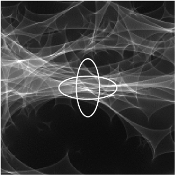
Figure 10: Illustration of why microlensing magnifications depend on the orientation of an elliptical source. Both ellipses have semimajor axes with lengths $a=R_{E}(\bar{m})$ and ellipticities $e=0.6$.

Figure 11: Dispersion in log $|\mu|$ versus source size for a positive parity image with different ellipticities and position angles. Rows show $e$=0.3, 0.6, and 0.9, while columns show PA=0, 30, 60 and 90 degrees. Solid and dashed curves have a uniform source profile. The solid curve shows a uniform mass function ($m_{1}/m_{2}=1$) and the dashed curve shows a Salpeter mass function with $m_{1}/m_{2}=0.1$. Dotted and dot-dashed curves have a Gaussian profile. The dotted line shows a uniform mass function, while the dot-dashed line shows a Salpeter mass function.

We now allow the source to be non-circular. This possibility has not been considered in previous microlensing analyses, although it is an important physical effect (see Kochanek et al., 2006). For a population of thin disks with random inclinations, a face-on source is rare; the average projected ellipticity is ${\bar{e}}=0.5$. Therefore, models of microlensing need to allow a non-circular shape for the source. This is certainly true for continuum microlensing, whose source is presumably a thin accretion disk. It may be true for broad-line microlensing as well, given evidence that BLRs may have some disky structure (e.g., Murray & Chiang, 1998; Elvis, 2000; Richards et al., 2004).

Figure 9 shows how the magnification dispersion depends on the ellipticity, $e\equiv 1-q$, and position angle, PA, of the source. In each panel we see that the dispersion increases monotonically with position angle, an effect which becomes more pronounced for large ellipticities. To understand this behaviour, first note that PA=$0^{\circ}$ describes a source whose major axis is orthogonal to the direction of shear, which defines the long axis of the caustics. An extended source with PA=$0^{\circ}$ is likely to cover one or more caustics regardless of where it is centered (see Figure 10). Small changes in the source position do not produce dramatic changes in the magnification. By contrast, for a source with PA=$90^{\circ}$ (aligned with the caustics), small displacements of the source can change the number of caustics covered, with corresponding large deviations in the magnification. This explains why the magnification dispersion is higher for sources aligned with the caustics (PA=$90^{\circ}$) than for orthogonal sources (PA=$0^{\circ}$). These effects become even more pronounced for more highly elongated sources.

In Figure 11 most of the effects discussed so far are considered simultaneously. As in Figure 5, the dispersion is larger for our fiducial model ($m_{1}/m_{2}=0.1$, dashed and dot-dashed curves) than for a uniform mass function (solid and dotted curves). As in Figure 8, the dispersion is smaller for the Gaussian profile (dotted and dot-dashed curves) than for the uniform source profile (solid and dashed curves). Perhaps the most interesting point is that as the source ellipticity increases, the difference between the four curves becomes smaller, i.e., the dispersion becomes even less sensitive to the mass function and source profile.

3.5 Accretion Disk Geometry

Finally, we consider whether variations in accretion disk geometry result in observable differences for microlensing. We model the source as an annulus with a given half-light radius, $r_{S}$, and hole-to-total area ratio, $Q^{2}$. This approach is useful in two ways. First, quasar accretion disks have inner radii defined by the innermost stable circular orbit of a particle in motion around the central black hole. Second, typical models (e.g., the Shakura-Sunyaev disk), emit over a wide range of wavelengths. Roughly distinct annular regions within the disk are revealed by observations in different bands (see, e.g., Mortonson, Schechter & Wambsganss, 2005). It is important to determine whether microlensing can be used to find the mass of the central black hole or the scale of the annulus within the disk emitting at some wavelength.

Figure 12: Dispersion in log $|\mu|$ versus source size for a positive parity image with different disk geometries. The source is modeled as an annulus with a given half-light radius. The solid, dotted, dashed and dot-dashed curves have hole-to-total area ratios, $Q^{2}=$ 0.01, 0.1, 0.5 and 0.9, respectively.

For simplicity we focus on a uniform source. Figure 12 shows the dispersion versus source size for disks with $Q^{2}$ = 0.01 (solid curve), 0.1 (dotted), 0.5 (dashed), and 0.9 (dot-dashed). For small sources ($r_{S}\la 1.5$) the dispersion is nearly identical for all values of $Q^{2}$. For larger sources, the dispersion remains similar for $Q^{2}=0.01$ and for $Q^{2}=0.1$. However, the cases $Q^{2}=0.5$ and $Q^{2}=0.9$ have larger dispersions, suggesting that only large holes can significantly affect microlensing.

3.6 Light Curves

While our analysis has focused on magnification distributions, microlensing has a time domain as well and we would like to understand whether variability timescales can provide more information about the lens and source. Although a complete study of microlensing light curves and light curve statistics is beyond the scope of this paper, we can examine sample light curves and begin to identify useful results. We have found that source ellipticity and orientation have pronounced effects on the magnification distribution, so we now see how they affect light curves.

To obtain sample light curves, we move the source through the magnification map along some trajectory, as shown in Figure 13. The natural time scale is the Einstein crossing time, $t_{E}=R_{E}({\bar{m}})/v_{\perp}$, where $v_{\perp}$ is the relative transverse velocity between the lens and source. Figure 14 (left) shows the resulting light curves for a source with $r_{S}$ = 1 and the same set of ellipticities and orientations used in Figure 9. Increasing either the ellipticity or the position angle increases the amount of variability, especially on short timescales. This is consistent with our previous interpretation: small changes to the source position have more effect when the source is aligned with the shear (PA=$90^{\circ}$) than when the source is perpendicular (PA=$0^{\circ}$). This can lead to a striking amount of rapid variability for highly flattened sources.

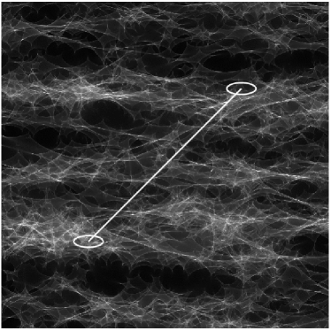
Figure 13: Construction of light curves. A source with ellipticity $e=0.6$ and PA$=90^{\circ}$ is moved along the trajectory from lower left to upper right. The resulting light curves are shown in the middle panel of the left column of Figure 14.

To quantify the amount of variability on different timescales, we follow Lewis & Irwin (1996) and use the structure function as a statistical measure of temporal variability. The structure function is defined to be the mean square change in the brightness after time $\Delta t$: $S(\Delta t)=\langle[M(t+\Delta t)-M(t)]^{2}\rangle$ where $M$ is the apparent magnitude and the average is over $t$. To obtain statistically meaningful results, we average the structure function over 100 realizations of light curves for a given set of parameters.

Figure 14: Light curves (left) and structure functions (right) for models with $e$= 0.3, 0.6 and 0.9 (top to bottom). Solid, dotted, dashed and dot-dashed curves have PA = 0, 30, 60 and 90 degrees, respectively.

The structure functions are shown in Figure 14 (right). They all have a roughly linear rise to a plateau beginning around $\Delta t/t_{E}\sim 5$. They confirm that there is more variability on shorter timescales when the source is elongated and/or aligned with the shear. It is customary to define a characteristic variability time scale as the interval at which the structure function reaches half its plateau value (see Lewis & Irwin, 1996; Schechter et al., 2003). We see that this time scale can vary by a factor of $\sim$2 depending on the ellipticity and orientation of the source.

The important implication is that elongated sources can lead to more rapid variability than circular sources that have identical half-light radii; this effect must be taken into account when interpreting observed variability timescales. It is not clear whether source shape can explain the rapid variability observed by Schechter et al. (2003) and Paraficz et al. (2006), but it should at least be considered as a possible alternative to relativistic motion.

4 Conclusions

We have presented a systematic study of microlensing of finite sources. We have extended earlier work by combining an finite source with a lens described by a stellar mass function. Following Mortonson, Schechter & Wambsganss (2005) we have explored how the surface brightness profile and geometry of the source affect microlensing (§3.3 and §3.5). We find that both effects are of minimal importance although subtle differences are apparent: making the source surface brightness profile steeper (Fig.8) and introducing a large hole in the source (Fig.12) both increase the magnification dispersion.

The mass function can play a more significant role. Although the slope of the mass function does not lead to noticeable changes in the magnification dispersion, the dynamic range can be important. The dispersion for a finite source becomes larger as the mass range increases. This result has been seen before for a broad bimodal mass function (Schechter, Wambsganss & Lewis, 2004; Lewis & Gil-Merino, 2006), but we have demonstrated it for a continuous and relatively narrow mass function as would be appropriate for stars. This raises the possibility of using microlensing to determine the dynamic range of stellar mass functions in distant galaxies.

Our discussion of dark matter in §3.2 reveals many interesting results. We find that the monotonic increase in dispersion for a point source lensed by a mixture of stars and dark matter (Schechter & Wambsganss, 2002) extends to the case of combining a small finite source with a power-law mass distribution. However, for moderately large sources we find that microlensing becomes less pronounced as the dark matter mass fraction is increased. As in previous studies (e.g., Schechter & Wambsganss, 2002), we find multiple peaks in the magnification histograms for moderate dark matter fractions. We also see that negative parity images have tails to low magnifications (see Schechter & Wambsganss, 2002), but only when the source is small.

Finally, we have for the first time considered non-circular sources with a range of position angles. We find that sources aligned with the shear have larger magnification dispersions than sources orthogonal to the shear. We suggest that an aligned source is much more sensitive to the position relative to caustics than an orthogonal source.

Apart from source size, which is fundamentally important, we believe that two of the effects we have identified have important physical implications. First, the continuum and BLR will be very different in their sensitivity to dark matter near a lensed image, particularly a negative-parity image. Thus, attempts to measure the dark matter content of galaxies with microlensing (see Schechter & Wambsganss, 2004) would greatly benefit from spectroscopic observations (see Keeton et al., 2006). Second, elliptical sources, which are relevant for inclined disks, may experience much more rapid variability than circular sources. This effect will surely be important when interpreting microlensing variability time scales.

References

- Abajas et al. (2002) Abajas C., Mediavilla E., Muñoz J. A., Popovic L. C., Oscoz A., 2002, ApJ, 576, 640
- Dalal & Kochanek (2002) Dalal N., Kochanek C. S., 2002, ApJ, 572, 25
- Dobler, Keeton & Wambsganss (2006) Dobler G., Keeton C., Wambsganss, J., astro-ph/0507522
- Elvis (2000) Elvis M., 2000, ApJ, 545, 63
- Gerhard (2006) Gerhard O., 2006, Planetary Nebulae Beyond the Milky Way, ESO Astrophysics Symposia, European Southern Observatory. Springer, p. 299
- Granot, Schechter & Wambsganss (2003) Granot J., Schechter P. L., Wambsganss J., 2003, ApJ, 583, 575
- Jaroszyński, Wambsganss & Paczyński (1992) Jaroszyński M., Wambsganss J., Paczyński B., 1992, ApJ, 396, L65
- Keeton et al. (2006) Keeton C. R., Burles S., Schechter P. L., Wambsganss J., 2006, ApJ, 639, 1
- Kochanek (2004) Kochanek C. S., 2004, ApJ, 605, 58
- Kochanek et al. (2006) Kochanek C. S., Dai X., Morgan C., Morgan N., Poindexter S., Chartas G., 2006, astro-ph/0609112
- Lewis & Gil-Merino (2006) Lewis G. F., Gil-Merino R., 2006, ApJ, 645, 835
- Lewis & Irwin (1996) Lewis G. F., Irwin M. J., 1996, MNRAS, 283, 225
- Metcalf & Madau (2001) Metcalf R. B., Madau P., 2001, ApJ, 563, 9
- Mortonson, Schechter & Wambsganss (2005) Mortonson M. J., Schechter P. L., Wambsganss J., 2005, ApJ, 628, 594
- Murray & Chiang (1998) Murray N., Chiang J., 1998, ApJ, 494, 125
- Paraficz et al. (2006) Paraficz D., Hjorth J., Burud I., Jakobsson P., Elíasdóttir Á., 2006, A&A, 455, L1
- Peterson & Horne (2005) Peterson B. M., Horne, K., 2005, in Planets to Cosmology: Essential Science in the Final Years of the Hubble Space Telescope (Space Telescope Science Institute Symposium Series) eds. Casertano S., Livio, M. Cambridge University Press: Cambridge, p.89
- Pooley et al. (2006) Pooley D., Blackburne J. A., Rappaport S., Schechter P., 2006, astro-ph/0607655
- Rauch et al. (1992) Rauch K., Mao S., Paczyński B., Wambsganss J., 1992, ApJ 386, 30
- Richards et al. (2004) Richards G. T. et al., 2004, ApJ, 610, 679
- Rusin & Kochanek (2005) Rusin D., Kochanek C.S., 2005, ApJ, 623, 666
- Schechter et al. (2003) Schechter P. L. et al., 2003, ApJ, 584, 657
- Schechter & Wambsganss (2002) Schechter P. L., Wambsganss J., 2002, ApJ, 580, 685
- Schechter & Wambsganss (2004) Schechter P. L., Wambsganns J., 2004, IAU Symposium no. 220, Eds: S. D. Ryder, D. J. Pisano, M. A. Walker, and K. C. Freeman. San Francisco: Astron. Soc. of the Pacific, p.103
- Schechter, Wambsganss & Lewis (2004) Schechter P. L., Wambsganss J., Lewis, G. F., 2004, ApJ, 613, 77
- Schneider & Wambsganss (1990) Schneider P., Wambsganss J., 1990, A&A, 237, 42
- Shakura & Sunyaev (1973) Shakura N. I., Sunyaev R. A. 1973, A&A, 24, 337
- Spekkens, Giovanelli & Haynes (2005) Spekkens K., Giovanelli R., Haynes M. P., 2005, AJ, 129, 2119
- Treu & Koopmans (2004) Treu T., Koopmans L.V.E., 2004, ApJ, 611, 739
- Treu et al. (2006) Treu T., Koopmans L.V.E., Bolton A.S., Burles S., Moustakas L.A., 2006, ApJ, 640, 662
- Wambsganss (1992) Wambsganss J., 1992, ApJ, 386, 19
- Wambsganss (1999) Wambsganss J., 1999, JCAM, 109, 353
- Wambganss, Paczyński & Schneider (1990) Wambsganss J., Paczyński B., Schneider P., 1990, ApJ, 358, L33
- Woźniak et al. (2000) Woźniak P. R., Udalski A., Szymański M., Kubiak M., Pietrzyński G., Soszyński I., Żebruń K., 2000, ApJ, 540, L65
- Wyithe, Agol & Fluke (2002) Wyithe J. S. B., Agol E., Fluke C. J. 2002, MNRAS, 331, 1041
- Wyithe & Turner (2001) Wyithe J. S. B., Turner E. L., 2001, MNRAS, 320, 21