Fe XIII emission lines in active region spectra obtained with the Solar Extreme-Ultraviolet Research Telescope and Spectrograph

Abstract

Recent fully relativistic calculations of radiative rates and electron impact excitation cross sections for Fe xiii are used to generate emission-line ratios involving 3s²3p²–3s3p³ and 3s²3p²–3s²3p3d transitions in the 170–225 Å and 235–450 Å wavelength ranges covered by the Solar Extreme-Ultraviolet Research Telescope and Spectrograph (SERTS). A comparison of these line ratios with SERTS active region observations from rocket flights in 1989 and 1995 reveals generally very good agreement between theory and experiment. Several new Fe xiii emission features are identified, at wavelengths of 203.79, 259.94, 288.56 and 290.81 Å. However, major discrepancies between theory and observation remain for several Fe xiii transitions, as previously found by Landi (2002) and others, which cannot be explained by blending. Errors in the adopted atomic data appear to be the most likely explanation, in particular for transitions which have 3s²3p3d ¹D₂ as their upper level. The most useful Fe xiii electron density diagnostics in the SERTS spectral regions are assessed, in terms of the line pairs involved being (i) apparently free of atomic physics problems and blends, (ii) close in wavelength to reduce the effects of possible errors in the instrumental intensity calibration, and (iii) very sensitive to changes in N_e over the range 10⁸–10¹¹ cm^-3. It is concluded that the ratios which best satisfy these conditions are 200.03/202.04 and 203.17/202.04 for the 170–225 Å wavelength region, and 348.18/320.80, 348.18/368.16, 359.64/348.18 and 359.83/368.16 for 235–450 Å.

1 Introduction

This is the latest in a series of papers in which we compare theoretical emission-line intensity ratios, generated using accurate atomic physics data for energy levels, radiative rates, and electron impact excitation cross sections, with high resolution spectra from the Solar Extreme-Ultraviolet Research Telescope and Spectrograph (SERTS). The major aim of our work is to investigate the importance of blending in the solar extreme-ultraviolet spectral regions covered by SERTS (170–225 Å; 235–450 Å), and hence determine which emission lines provide the most reliable diagnostics, and also where possible to identify new emission features. To date, we have studied the SERTS spectra of C iv (Keenan et al. 1993), Mg ix (Keenan et al. 1994), Si x (Keenan et al. 2000a), S xi (Keenan et al. 2000b), Mg vi (Keenan et al. 2002), Si ix (Keenan et al. 2003a), Si viii (Keenan et al. 2004), Na-like ions between Ar viii and Zn xx (Keenan et al. 2003b), and the iron ions Fe xi (Pinfield et al. 2001; Keenan et al. 2005a), Fe xii (Keenan et al. 1996) and Fe xv (Keenan et al. 2005b).

Our work is currently of particular relevance due to the recent launch of the Hinode mission. This has on board the EUV Imaging Spectrometer (EIS), which obtains high spectral resolution observations over wavelength ranges similar to those covered by SERTS, specifically 170–210 Å and 250–290 Å (Culhane et al. 2005). Clearly, it is important that the emission lines observed by the EIS are investigated in detail and the best diagnostics identified, with SERTS providing the ideal testbed for this. In the present paper we undertake a study of Fe xiii, which as noted by Young, Landi & Thomas (1998) is the species with the most emission lines detected in the SERTS spectral range. It has also long been known that Fe xiii emission lines provide very useful electron density diagnostics for solar plasmas (Flower & Nussbaumer 1974).

The most detailed investigation to date of the Fe xiii solar extreme-ultraviolet spectrum, which also employs SERTS observations, is probably that by Landi (2002). In addition, his paper contains an excellent review of previous work on Fe xiii. Landi undertook two separate calculations of theoretical line ratios for Fe xiii, with the most reliable consisting of a 27 fine-structure level model ion, comprising the 3s²3p², 3s3p³ and 3s²3p3d configurations, with radiative rates being taken from the SUPERSTRUCTURE calculations of Young (2004), and electron impact excitation cross sections from the R-matrix results of Gupta & Tayal (1998). However, Landi found that some of the Fe xiii line intensities showed large discrepancies between theory and observation, which could not be explained by blending, and was therefore most likely due to errors in the adopted atomic data (see also Young et al. 1998 and Landi & Landini 1997).

More recently, Aggarwal & Keenan (2004, 2005) have employed the relativistic GRASP and Dirac R-matrix codes to calculate radiative rates and electron impact excitation cross sections, respectively, for all transitions among the energetically lowest 97 fine-structure levels of Fe xiii. In this paper we use these data to generate theoretical emission-line ratios for Fe xiii, and compare these with SERTS observations, to (i) investigate if previous discrepancies between theory and observation may be resolved, (ii) assess the importance of blending in the SERTS observations, (iii) detect new Fe xiii emission lines, and finally (iv) identify the best Fe xiii line pairs for use as electron density diagnostics.

2 Observational data

The first fully successful SERTS flight was on 1989 May 5 (Neupert et al. 1992; Thomas & Neupert 1994), and carried a standard gold-coated toroidal diffraction grating. It observed active region NOAA 5464 and detected hundreds of first-order emission lines in the 235–450 Å wavelength range, as well as dozens of features spanning 170–225 Å, which appeared in second-order among the 340–450 Å first-order lines. The spectrum was recorded on Kodak 101–07 emulsion, at a spectral resolution of 50–80 mÅ (FWHM) in first-order, and a spatial resolution of approximately 7 arcsec (FWHM).

SERTS had additional technology-demonstration flights in 1991 and 1993 (Brosius et al. 1996), carrying a multilayer-coated diffraction grating that enhanced the instrumental sensitivity over a limited range of its first-order bandpass. However, over much of the range, these observations are actually at a somewhat reduced sensitivity compared to the 1989 data. As a result, fewer emission lines were detected, and many of those that were measured had larger uncertainities (see, for example, the comparison of SERTS 1989, 1991 and 1993 measurements in Keenan et al. 2003a,b and Keenan et al. 2005b). Consequently, the 1989 observations (henceforth referred to as SERTS–89) provide the best SERTS spectrum for investigating emission features in the first-order wavelength range 235–450 Å, and are hence employed in the present analysis.

During a rocket flight on 1995 May 15, SERTS observed active region NOAA 7870, once again recording the spectrum on Kodak 101–07 emulsion at a spatial resolution of approximately 5 arcsec (Brosius, Davila & Thomas 1998). However, this version of the instrument incorporated a multilayer-coated toroidal diffraction grating that enhanced its sensivitity to second-order features in the 170–225 Å wavelength range. This led to the detection of many second-order emission lines not seen on previous SERTS flights (Thomas & Neupert 1994; Brosius et al. 1996), and furthermore provided the highest spectral resolution (0.03 Å) ever achieved for spatially resolved active region spectra in this wavelength range. The SERTS 1995 active region spectrum (henceforth SERTS–95) therefore provides the best observations for investigating emission lines in the 170–225 Å region, and is employed in the present paper. Further details of the observations, and the wavelength and absolute flux calibration procedures employed in the data reduction, may be found in Brosius et al. (1998). Similar information for the SERTS–89 spectrum is available from Thomas & Neupert (1994). We note that the SERTS spectra have been calibrated using temperature and density insensitive emission line ratios, including those from Fe xiii. As the relevant line ratio calculations may have changed since these calibrations were performed, and indeed several have (see, for example, Keenan et al. 2005b), any comparison of theoretical and observed Fe xiii line ratios must be treated with some caution. However, even if the calibration were to change, this would be unlikely to significantly affect line pairs which are close in wavelength.

We have searched for Fe xiii emission lines in the SERTS–89 and SERTS–95 spectra using the identifications of Thomas & Neupert (1994) and Brosius et al. (1998), as well as other sources including the NIST database, the latest version (V5.2) of the chianti database (Dere et al. 1997; Landi et al. 2006), and previous solar detections where available (for example, those of Dere 1978). In Tables 1 and 2 we list the Fe xiii transitions found in the SERTS–95 and SERTS–89 spectra, respectively, along with the measured wavelengths. We also indicate possible blending lines or alternative identifications as suggested by Brosius et al. or Thomas & Neupert in their original line lists for these observations. Note that we list two measured wavelengths for the same 3s²3p^{2 3}P₁–3s²3p3d ³P₀ transition in the SERTS–95 spectrum, namely 202.43 and 203.17 Å. Brosius et al. identify Fe xiii lines at 202.42 and 203.16 Å in the SERTS–95 data, but Landi (2002) only lists the 203.16 Å emission feature (as does chianti). We return to the identification of this line in Section 4.1.

Table 1: Fe xiii line identifications in the second-order SERTS 1995 active region spectrum.

Wavelength (Å)	Transition	Notea
196.53	3s23p2 1D2–3s23p3d 1F3
200.03	3s23p2 3P1–3s23p3d 3D2
201.13	3s23p2 3P1–3s23p3d 3D1	Blended with Fe xii lineb
202.04	3s23p2 3P0–3s23p3d 3P1
202.43	3s23p2 3P1–3s23p3d 3P0
203.17	3s23p2 3P1–3s23p3d 3P0	Identified as this transition by Landi (2002)
203.79	3s23p2 3P2–3s23p3d 3D2	No line listed
203.83	3s23p2 3P2–3s23p3d 3D3	Listed with 203.79 Å as a single feature
204.26	3s23p2 3P1–3s23p3d 1D2
204.95	3s23p2 3P2–3s23p3d 3D1
208.67	3s23p2 1S0–3s23p3d 1P1	No line listed; identified as Ca xv by Dere (1978)
209.63	3s23p2 3P1–3s23p3d 3P2
209.91	3s23p2 3P2–3s23p3d 3P1
213.77	3s23p2 3P2–3s23p3d 3P2
216.90	3s23p2 1D2–3s23p3d 3D2,3	Blended with Si viii line
221.82	3s23p2 1D2–3s23p3d 1D2

^aFrom Brosius et al. (1998).

^bFrom Thomas & Neupert (1994).

Table 2: Fe xiii line identifications in the first-order SERTS 1989 active region spectrum.

Wavelength (Å)	Transition	Notea
240.72	3s23p2 3P0–3s3p3 3S1
246.20	3s23p2 3P1–3s3p3 3S1
251.94	3s23p2 3P2–3s3p3 3S1
256.43	3s23p2 1D2–3s3p3 1P1	Blended with Zn xx line
259.94	3s23p2 1D2–3s23p3d 3F2	Unidentified line
272.21	3s23p2 1D2–3s3p3 3S1	Unidentified line
288.56	3s23p2 1S0–3s3p3 1P1	No line listedb
290.81	3s23p2 3P2–3s3p3 1D2	No line listed
311.57	3s23p2 3P1–3s3p3 3P2
312.17	3s23p2 3P1–3s3p3 3P1
312.89	3s23p2 3P1–3s3p3 3P0	Unidentified linec
318.12	3s23p2 1D2–3s3p3 1D2
320.80	3s23p2 3P2–3s3p3 3P2
321.46	3s23p2 3P2–3s3p3 3P1
348.18	3s23p2 3P0–3s3p3 3D1
359.64	3s23p2 3P1–3s3p3 3D2
359.83	3s23p2 3P1–3s3p3 3D1
368.16	3s23p2 3P2–3s3p3 3D3	Blended with Cr xiii line
413.00	3s23p2 1D2–3s3p3 3D3

^aFrom Thomas & Neupert (1994).

^bListed by Brosius et al. (1998) as an unidentified feature.

^cSubsequently identified by Brickhouse et al. (1995).

Intensities and observed line widths (FWHM) of the Fe xiii features are given in Tables 3 and 4 for the SERTS–95 and SERTS–89 datasets, respectively, along with the associated 1$\sigma$ errors. These were measured using modified versions of the Gaussian fitting routines employed by Thomas & Neupert (1994). Specifically, we have incorporated the ability to filter spectral noise at low intensities. By utilizing fitted Gaussian exponents around the line centre, it is possible to extrapolate wavelength and intensity values away from the emission line core, thus removing any artefacts associated with noise spikes and/or hot pixels which may affect the unfiltered spectral profile. The intensities, FWHM values and their uncertainties listed in Tables 3 and 4 are hence somewhat different from those originally reported in Thomas & Neupert and Brosius et al. (1998). Also, a uniform factor of 1.24 has been applied here to all SERTS–89 intensities, reflecting a more recent re-evaluation of its absolute calibration scale. Even so, in all directly comparable cases, the resulting line intensity values usually differ only slightly from those obtained using previously published data. The listed line widths include an instrumental broadening component due to the spectrometer optics, and so should be considered as only upper limits to the actual widths of the lines.

Table 3: Fe xiii line intensities and widths from the SERTS 1995 active region spectrum.

Wavelength	Intensity	Line width
(Å)	(erg cm-2 s-1 sr-1)	(mÅ)
196.53	134.5 $\pm$ 33.1	42 $\pm$ 7
200.03	305.0 $\pm$ 35.6	47 $\pm$ 4
201.13	469.4 $\pm$ 59.8	49 $\pm$ 3
202.04	1219.1 $\pm$ 135.6	49 $\pm$ 3
202.43	73.6 $\pm$ 17.1	38 $\pm$ 4
203.17	155.8 $\pm$ 23.9	37 $\pm$ 3
203.79	310.2 $\pm$ 43.9	46 $\pm$ 3
203.83	1547.2 $\pm$ 169.8	54 $\pm$ 4
204.26	192.0 $\pm$ 27.7	46 $\pm$ 5
204.95	268.7 $\pm$ 42.5	63 $\pm$ 6
208.67	44.6 $\pm$ 13.5	25 $\pm$ 5
209.63	210.1 $\pm$ 33.6	44 $\pm$ 4
209.91	236.7 $\pm$ 41.5	63 $\pm$ 7
213.77	93.8 $\pm$ 20.4	35 $\pm$ 4
216.90	54.3 $\pm$ 15.9	32 $\pm$ 4
221.82	219.4 $\pm$ 30.9	30 $\pm$ 3

Table 4: Fe xiii line intensities and widths from the SERTS 1989 active region spectrum.

Wavelength	Intensity	Line width
(Å)	(erg cm-2 s-1 sr-1)	(mÅ)
240.72	156.6 $\pm$ 60.3	74 $\pm$ 20
246.20	140.7 $\pm$ 41.7	42 $\pm$ 6
251.94	447.8 $\pm$ 66.3	84 $\pm$ 6
256.43	176.0 $\pm$ 63.4	96 $\pm$ 28
259.94	49.2 $\pm$ 19.8	30 $\pm$ 8
272.21	82.5 $\pm$ 19.2	50 $\pm$ 9
288.56	18.0 $\pm$ 8.2	45 $\pm$ 11
290.81	6.1 $\pm$ 3.2	25 $\pm$ 10
311.57	37.4 $\pm$ 11.8	66 $\pm$ 13
312.17	104.7 $\pm$ 10.4	87 $\pm$ 5
312.89	57.7 $\pm$ 16.0	42 $\pm$ 8
318.12	108.5 $\pm$ 14.0	99 $\pm$ 8
320.80	212.8 $\pm$ 27.2	95 $\pm$ 6
321.46	41.8 $\pm$ 9.1	83 $\pm$ 10
348.18	158.2 $\pm$ 18.7	90 $\pm$ 5
359.64	182.9 $\pm$ 20.4	91 $\pm$ 5
359.83	27.9 $\pm$ 5.4	77 $\pm$ 8
368.16	167.2 $\pm$ 29.9	83 $\pm$ 11
413.00	8.8 $\pm$ 2.5	120 $\pm$ 15

We plot portions of the SERTS–89 and SERTS–95 spectra containing Fe xiii features in Figs 1–5, to show the quality of the observational data. In particular, we have been able to identify both the 203.79 and 203.83 Å lines of Fe xiii (Fig. 2), which previously have been listed as a single feature (see, for example, Brosius et al. 1998). We note that each SERTS spectrum exhibits a background level due to film fog, scattered light and actual solar continuum. The background was calculated using methods detailed in Thomas & Neupert (1994) and Brosius et al., and then subtracted from the initial spectrum, leaving only an emission line spectrum (with noise) on a zero base level. It is this zero base level which is shown in Figs 1–5. We note that some of the measured Fe xiii emission lines, such as the 288.56 Å transition (Fig. 4), have line intensities comparable to the noise fluctuations. In these instances the reality of the line was confirmed by a visual inspection of the original SERTS film.

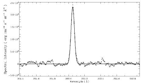
Figure 1: Plot of the SERTS 1995 active region spectrum in the 201.4–202.9 Å wavelength range. The profile fit to the Fe xiii 202.04 Å feature is shown by a solid line.

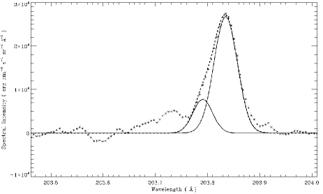
Figure 2: Plot of the SERTS 1995 active region spectrum in the 203.5–204.0 Å wavelength range. The profile fit to the Fe xiii 203.79 and 203.83 Å features is shown by a dashed line, while the fits for the individual components are shown by solid lines. Also clearly visible in the figure is an unidentified feature at 203.73 Å.

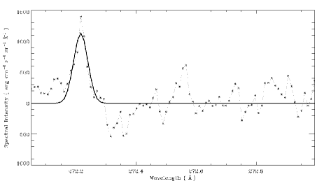
Figure 3: Plot of the SERTS 1989 active region spectrum in the 272.1–272.9 Å wavelength range. The profile fit to the Fe xiii 272.21 Å feature is shown by a solid line.

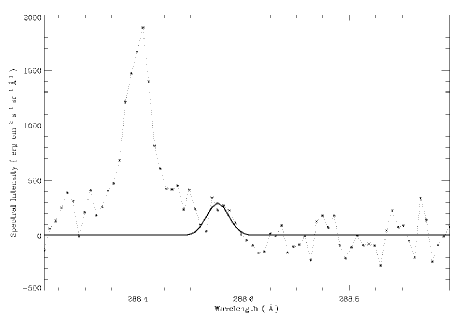
Figure 4: Plot of the SERTS 1989 active region spectrum in the 288.3–288.9 Å wavelength range. The profile fit to the Fe xiii 288.56 Å feature is shown by a solid line. Also clearly visible in the figure is the S xii 288.40 Å line.

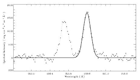
Figure 5: Plot of the SERTS 1989 active region spectrum in the 320.1–321.2 Å wavelength range. The profile fit to the Fe xiii 320.80 Å feature is shown by a solid line. Also clearly visible in the figure is the Ni xviii 320.56 Å line.

3 Theoretical line ratios

The model ion for Fe xiii consisted of the 97 energetically lowest fine-structure levels, which are listed in Table 1 of Aggarwal & Keenan (2004), and include levels from the 3s²3p², 3s3p³, 3s²3p3d, 3p⁴, 3s3p²3d and 3s²3d² configurations. Experimental energy levels, which are only available for a small number (22) of Fe xiii states, were obtained from the NIST database. For the remaining values the theoretical results of Aggarwal & Keenan (2004) were adopted.

The electron impact excitation cross sections employed in the present paper are the fully relativistic Dirac R-matrix code calculations of Aggarwal & Keenan (2005). For Einstein A-coefficients, Aggarwal & Keenan (2004) undertook two calculations with the fully relativistic grasp code, namely one considering the 97 fine-structure levels from the 6 configurations listed above (termed GRASP6), and another with 301 levels from the 13 configurations 3s²3p², 3s3p³, 3s²3p3d, 3p⁴, 3s3p²3d, 3s²3d², 3p³3d, 3s3p3d², 3s3d³ and 3s²3p4$\ell$ (GRASP13). Aggarwal & Keenan noted that the GRASP13 results represent a significant improvement over the GRASP6 data, and they have therefore been adopted in the present paper. Unfortunately however, Aggarwal & Keenan only published their GRASP6 results, and hence in Tables 5 and 6 we provide the GRASP13 calculations for all 4656 transitions among the 97 levels considered in our model ion. Complete versions of these tables are available in the electronic version of the paper, with only sample results presented in the hardcopy edition. The indices used to represent the lower and upper levels of a transition have been defined in Table 1 of Aggarwal & Keenan. We note that radiative data for all 45150 transitions among the 301 levels considered in our GRASP13 calculations are available in electronic form on request from one of the authors (K.Aggarwal@qub.ac.uk).

Table 5: Transition energies/wavelengths ($\lambda_{ij}$ in $\AA$), radiative rates (A_ji in s^-1), oscillator strengths (f_ij, dimensionless), and line strengths (S, in atomic units) for a sample of electric dipole (E1) and magnetic quadrupole (M2) transitions in Fe xiii. ($a{\pm}b\equiv a{\times}$10^±b).

$i$	$j$	$\lambda_{ij}$	A${}^{{\rm E1}}_{ji}$	f${}^{{\rm E1}}_{ij}$	SE1	A${}^{{\rm M2}}_{ji}$	f${}^{{\rm M2}}_{ij}$	SM2
1	6	4.802$+$02	0.000$+$00	0.000$+$00	0.000$+$00	5.771$-$01	9.975$-$11	4.941$+$00
1	7	3.505$+$02	1.224$+$09	6.763$-$02	7.804$-$02	0.000$+$00	0.000$+$00	0.000$+$00
1	8	3.503$+$02	0.000$+$00	0.000$+$00	0.000$+$00	3.193$+$00	2.937$-$10	5.647$+$00
1	11	3.040$+$02	1.262$+$09	5.244$-$02	5.248$-$02	0.000$+$00	0.000$+$00	0.000$+$00
1	12	3.034$+$02	0.000$+$00	0.000$+$00	0.000$+$00	1.292$+$00	8.919$-$11	1.115$+$00
1	13	2.754$+$02	0.000$+$00	0.000$+$00	0.000$+$00	4.536$+$00	2.579$-$10	2.410$+$00
1	14	2.306$+$02	0.000$+$00	0.000$+$00	0.000$+$00	5.677$+$00	2.263$-$10	1.241$+$00
1	15	2.367$+$02	7.507$+$09	1.892$-$01	1.475$-$01	0.000$+$00	0.000$+$00	0.000$+$00
1	18	2.241$+$02	8.513$+$08	1.923$-$02	1.419$-$02	0.000$+$00	0.000$+$00	0.000$+$00
1	19	2.023$+$02	0.000$+$00	0.000$+$00	0.000$+$00	9.328$-$01	2.860$-$11	1.059$-$01
1	20	1.990$+$02	4.549$+$10	8.100$-$01	5.306$-$01	0.000$+$00	0.000$+$00	0.000$+$00
1	22	1.971$+$02	0.000$+$00	0.000$+$00	0.000$+$00	7.364$-$03	2.143$-$13	7.336$-$04
1	23	1.942$+$02	1.245$+$10	2.112$-$01	1.350$-$01	0.000$+$00	0.000$+$00	0.000$+$00
1	24	1.931$+$02	0.000$+$00	0.000$+$00	0.000$+$00	7.913$+$00	2.211$-$10	7.116$-$01
1	28	1.719$+$02	4.218$+$08	5.603$-$03	3.170$-$03	0.000$+$00	0.000$+$00	0.000$+$00

Table 6: Transition energies/wavelengths ($\lambda_{ij}$ in $\AA$), radiative rates (A_ji in s^-1)), oscillator strengths (f_ij, dimensionless), and line strengths (S, in atomic units) for a sample of electric quadrupole (E2) and magnetic dipole (M1) transitions in Fe xiii. ($a{\pm}b\equiv a{\times}$10^±b).

$i$	$j$	$\lambda_{ij}$	A${}^{{\rm E2}}_{ji}$	f${}^{{\rm E2}}_{ij}$	SE2	A${}^{{\rm M1}}_{ji}$	f${}^{{\rm M1}}_{ij}$	SM1
1	2	1.092$+$04	0.000$+$00	0.000$+$00	0.000$+$00	1.332$+$01	7.147$-$07	1.930$+$00
1	3	5.382$+$03	2.572$-$03	5.584$-$11	5.183$-$02	0.000$+$00	0.000$+$00	0.000$+$00
1	4	1.994$+$03	2.514$-$01	7.492$-$10	3.537$-$02	0.000$+$00	0.000$+$00	0.000$+$00
1	27	1.644$+$02	9.052$+$04	1.833$-$06	4.848$-$02	0.000$+$00	0.000$+$00	0.000$+$00
1	29	1.612$+$02	0.000$+$00	0.000$+$00	0.000$+$00	8.133$+$00	9.500$-$11	3.786$-$06
1	31	1.582$+$02	0.000$+$00	0.000$+$00	0.000$+$00	1.470$-$01	1.655$-$12	6.476$-$08
1	32	1.577$+$02	6.916$+$02	1.289$-$08	3.010$-$04	0.000$+$00	0.000$+$00	0.000$+$00
1	33	1.576$+$02	4.851$+$03	9.029$-$08	2.104$-$03	0.000$+$00	0.000$+$00	0.000$+$00
1	38	1.521$+$02	0.000$+$00	0.000$+$00	0.000$+$00	1.839$-$02	1.912$-$13	7.191$-$09
1	39	1.518$+$02	8.246$+$02	1.425$-$08	2.969$-$04	0.000$+$00	0.000$+$00	0.000$+$00
1	42	1.456$+$02	2.378$+$05	3.778$-$06	6.941$-$02	0.000$+$00	0.000$+$00	0.000$+$00
1	46	1.410$+$02	1.708$+$01	2.545$-$10	4.251$-$06	0.000$+$00	0.000$+$00	0.000$+$00
1	47	1.406$+$02	0.000$+$00	0.000$+$00	0.000$+$00	8.572$+$00	7.620$-$11	2.649$-$06
1	49	1.347$+$02	9.169$+$04	1.248$-$06	1.817$-$02	0.000$+$00	0.000$+$00	0.000$+$00
1	50	1.331$+$02	0.000$+$00	0.000$+$00	0.000$+$00	2.064$-$01	1.644$-$12	5.412$-$08

Proton impact excitation is only important for the fine-structure transitions among the ground-state 3s²3p^{2 3}P_0,1,2 levels. In the present paper we have employed the quantal calculations of Faucher (1975) as given in Faucher & Landman (1977).

Using the above atomic data, in conjunction with a recently updated version of the statistical equilibrium code of Dufton (1977), relative Fe xiii level populations and hence emission-line strengths were calculated for a grid of electron temperature (T_e) and density (N_e) values, with T_e = 10^6.0, 10^6.2 and 10^6.4 K, and N_e = 10⁸–10¹³ cm^-3 in steps of 0.1 dex. The adopted temperature range covers that over which Fe xiii has a fractional abundance in ionization equilibrium of N(Fe xiii)/N(Fe) $\geq$ 0.025 (Mazzotta et al. 1998), and hence should be appropriate to most coronal-type plasmas. Our results are far too extensive to reproduce here, as with 97 fine-structure levels in our calculations we have intensities for 4656 transitions at each of the 153 possible (T_e, N_e) combinations considered. However, results involving any line pair, in either photon or energy units, are freely available from one of the authors (FPK) by email on request. In addition, we note that we have Fe xiii atomic data for the electron temperature range T_e = 10^5.9–10^6.7 K in steps of 0.1 dex, and hence can quickly generate relative line strengths at additional temperatures, if requested.

In Figs 6–8 we plot some sample theoretical emission line ratios as a function of both T_e and N_e, to illustrate their sensitivity to the adopted plasma parameters. The transitions corresponding to the wavelengths given in the figures are listed in Tables 1 or 2. Given expected errors in the adopted atomic data of typically $\pm$20 per cent (see the references above), we would expect the theoretical ratios to be accurate to better than $\pm$30 per cent. An inspection of Figs 6–8 reveals that 203.83/202.04 is potentially a particularly good N_e–diagnostic, involving lines which are very close in wavelength, varying by a factor of 43 between N_e = 10⁸ and 10¹¹ cm^-3, and showing relatively little sensitivity to the adopted temperature. For example, changing T_e from 10^6.2 to 10^6.4 K (i.e. by 60 per cent) would lead to a less than 0.1 dex difference in the derived value of N_e over the density interval N_e = 10⁹–10¹¹ cm^-3. We discuss the usefulness of the Fe xiii transitions as density diagnostics in more detail in Section 4.3.

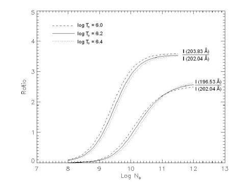
Figure 6: The theoretical Fe xiii emission line intensity ratios I(203.83 Å)/I(202.04 Å) and I(196.53 Å)/I(202.04 Å), where I is in energy units, plotted as a function of logarithmic electron density (N_e in cm^-3) at the temperature of maximum Fe xiii fractional abundance in ionization equilibrium, T_e = 10^6.2 K (Mazzotta et al. 1998), plus $\pm$0.2 dex about this value.

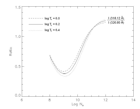
Figure 7: Same as Fig. 6 except for the I(318.12 Å)/I(320.80 Å) intensity ratio.

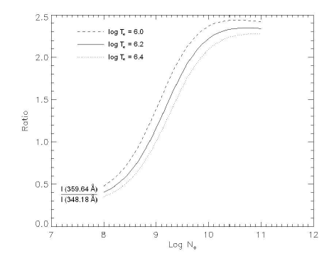
Figure 8: Same as Fig. 6 except for the I(359.64 Å)/I(348.18 Å) intensity ratio.

4 Results and discussion

Emission-line ratios may be categorised as 3 types, namely:

1. branching ratios, i.e. those which are predicted to be constant as the relevant transitions arise from common upper levels;

2. those which are predicted to be only weakly sensitive to the adopted electron temperature and density over the range of plasma parameters of interest;

3. those which are predicted to be strongly N_e–sensitive, and hence potentially provide useful diagnostics.

For a comparison of theory and observation, in order to identify blends and/or problems with atomic data, clearly the line ratios which fall into categories 1 and 2 are the most useful, as one does not need to reliably know the plasma electron temperature and density in order to calculate the line ratio. Accordingly, in Tables 7 and 8 we list a range of observed line ratios for the SERTS–95 and SERTS–89 active regions, respectively (along with the associated 1$\sigma$ errors), which fulfill the criteria for category 1 or 2. Also listed in the tables are the predicted theoretical ratios both from the present calculations and the latest version (V5.2) of the chianti database (Dere et al. 1997; Landi et al. 2006), which employs the 27-level model ion and atomic data discussed by Landi (2002). For category 2 ratios, we have defined ‘weakly sensitive’ as being those which are predicted to vary by less than $\pm$20 per cent when the electron density is changed by a factor of 2 (i.e. $\pm$0.3 dex). Electron density estimates for the SERTS–89 and SERTS–95 active regions from line ratios in species formed at similar temperatures to Fe xiii vary widely, with log N_e $\simeq$ 8.8–9.8 for SERTS–89 (Young et al. 1998) and log N_e $\simeq$ 9.0–9.7 for SERTS–95 (Brosius et al. 1998). However, most of the derived densities are consistent with log N_e = 9.4$\pm$0.3 for both active regions. The theoretical results in Tables 7 and 8 have therefore been calculated at the temperature of maximum Fe xiii fractional abundance in ionization equilibrium, T_e = 10^6.2 K (Mazzotta et al. 1998), and for N_e = 10^9.4 cm^-3. However we note that changing the adopted temperature by $\pm$0.2 dex or the density by $\pm$0.5 dex would not significantly alter the discussions below.

Table 7: Comparison of theory and observation for emission-line intensity ratios from the SERTS 1995 active region spectrum.

Line ratio	Observed	Present	chianti
		theory	theory
(i) Ratios of lines with common upper levels:
200.03/203.79	0.98 $\pm$ 0.18	0.84	0.73
201.13/204.95	1.7 $\pm$ 0.3	3.7	3.3
202.04/209.91	5.2 $\pm$ 1.1	5.1	6.7
204.26/221.82	0.88 $\pm$ 0.18	0.38	0.59
209.63/213.77	2.2 $\pm$ 0.6	1.1	1.0
(ii) Ratios which are only weakly Ne–dependent:a
200.03/201.13	0.65 $\pm$ 0.11	0.74	0.75
202.43/200.03	0.24 $\pm$ 0.06	0.49	0.53
203.17/200.03	0.51 $\pm$ 0.10	0.49	0.53
203.79/203.83	0.20 $\pm$ 0.04	0.32	0.33
204.26/200.03	0.63 $\pm$ 0.12	0.32	0.63
204.95/200.03	0.88 $\pm$ 0.17	0.37	0.40
208.67/200.03	0.15 $\pm$ 0.05	0.053	0.028
209.63/204.26	1.1 $\pm$ 0.2	2.9	1.2
209.63/221.82	0.96 $\pm$ 0.20	1.1	0.72
216.90/203.83	0.035 $\pm$ 0.011	0.074	0.10
216.90/213.77	0.58 $\pm$ 0.21	0.33	0.57

^aPresent theoretical ratios and those from chianti calculated at T_e = 10^6.2 K and N_e = 10^9.4 cm^-3.

Table 8: Comparison of theory and observation for emission-line intensity ratios from the SERTS 1989 active region spectrum.

Line ratio	Observed	Present	chianti
		theory	theory
(i) Ratios of lines with common upper levels:
240.72/246.20	1.1 $\pm$ 0.5	0.41	0.42
246.20/251.94	0.31 $\pm$ 0.10	0.53	0.52
256.43/288.56	9.8 $\pm$ 5.7	7.6	7.8
272.21/251.94	0.18 $\pm$ 0.05	0.018	0.018
290.81/318.12	0.056 $\pm$ 0.030	0.020	0.022
311.57/320.80	0.18 $\pm$ 0.06	0.14	0.13
321.46/312.17	0.40 $\pm$ 0.10	0.50	0.46
359.83/348.18	0.18 $\pm$ 0.04	0.25	0.25
413.00/368.16	0.053 $\pm$ 0.018	0.056	0.068
(ii) Ratios which are only weakly Ne–dependent:a
259.94/251.94	0.11 $\pm$ 0.05	0.10	0.016
272.21/256.43	0.47 $\pm$ 0.20	0.020	0.098
272.21/359.64	0.45 $\pm$ 0.12	0.025	0.11
288.56/359.64	0.098 $\pm$ 0.046	0.16	0.11
312.89/320.80	0.27 $\pm$ 0.08	0.24	0.28
318.12/368.16	0.65 $\pm$ 0.14	0.33	0.29
321.46/348.18	0.26 $\pm$ 0.06	0.30	0.31
359.83/312.17	0.27 $\pm$ 0.06	0.42	0.36
359.83/359.64	0.15 $\pm$ 0.03	0.15	0.27
368.16/359.64	0.91 $\pm$ 0.19	1.2	0.95

^aPresent theoretical ratios and those from chianti calculated at T_e = 10^6.2 K and N_e = 10^9.4 cm^-3.

4.1 SERTS–95 active region spectrum: transitions in the 170–225 Å wavelength range

In the SERTS–95 second-order spectral region, only 3s²3p²–3s²3p3d transitions of Fe xiii are detected, spanning the wavelength interval 196–222 Å (see Table 1). A comparison of the observed and theoretical 201.13/204.95 ratios from Table 7 indicate that the measured 204.95 Å line intensity is too strong, supported by the fact that the observed 204.95/200.03 ratio is much larger than the theoretical value. Also, the 200.03/201.13 ratio measurement is in good agreement with the present calculations and those from chianti, indicating that both the 200.03 and 201.13 Å lines are reliably detected and modelled. To identify possible blending species and assess their impact, we have generated a synthetic active region spectrum using chianti. However, no significant emission features are predicted by chianti close to 204.95 Å, apart from the Fe xiii line. Young et al. (1998) have suggested that the blending could be due to an unidentified first-order line at 409.90 Å, which would appear in second-order at 204.95 Å. Although chianti has no suitable blending species at this wavelength, the database of van Hoof lists the Fe v 3d^{4 3}F₂–3d³4p ³G₃ line, which could be a possibility. However, to properly assess this will need to await the calculation of accurate atomic data for Fe v and the inclusion of these in chianti. We also note that although Thomas & Neupert (1994) list the 201.13 Å line as being blended with an Fe xii transition, the chianti synthetic spectrum indicates that Fe xii is responsible for less than 3 per cent of the total line intensity, which is supported by the good agreement found here between theory and observation.

The good agreement between theory and observation for the 200.03/203.79 ratio confirms our identification of the 203.79 Å transition, the first time (to our knowledge) that this line has been detected separately from the 203.83 Å feature. Similarly, there is no discrepancy between theory and observation for the 202.04/209.91 ratio, indicating that both lines are reliably detected and free from problems. However, the experimental value of the 204.26/221.82 ratio is much larger than theory, with the discrepancy with the present calculations being larger than that with chianti. This could be due to blending, as the measured 204.26/200.03 ratio is also larger than theory, although in this instance there is good agreement with the chianti prediction. By contrast, the 209.63/221.82 experimental ratio shows a slightly smaller discrepancy with the present calculations, while the 209.63/204.26 measurement is lower than the present calculations and in better agreement with chianti. However, the measured 209.63/213.77 ratio disagrees with both the present calculations and those from chianti. Landi (2002) note problems with the 204.26, 209.63 and 221.82 Å lines, which cannot be due to blending and hence are still clearly unresolved by the present analysis.

The good agreement of the observed 203.17/200.03 ratio with theory, as opposed to the discrepancy found for 202.43/200.03, indicates that the 203.17 Å feature is the Fe xiii line. Although chianti does not list a possible identification for the 202.43 Å line, the list of van Hoof notes the presence of the Fe xv 3s3d ³D₃–3p3d ³F₂ transition at 404.84 Å, which could be the 202.43 Å feature in first-order. However, Keenan et al. (2005b) predicts the 404.84 Å line intensity to be only 2$\times$10^-5 that of Fe xv 417.25 Å, which has I = 420 erg cm^-2 s^-1 sr^-1 (Thomas & Neupert 1994). Hence Fe xv is far too weak to account for the observed feature at 202.43 Å. Interestingly however, we note that there is another Fe v transition in the database of van Hoof predicted to lie at 404.87 Å, namely 3d^{4 3}D₂–3d³4p ³D₁, which will appear in second-order at 202.44 Å.

The experimental 208.67/200.03 ratio is larger than theory, but our results indicate that Fe xiii contributes as much as 50 per cent to the 208.67 Å intensity, and the line is not due solely to Ca xv. This is in agreement with the chianti synthetic spectrum, which indicates that Fe xiii should be responsible for around 80 per cent of the total 208.67 Å intensity in an active region. However, we note that Ca xv is known to dominate this emission line in solar flares (Keenan et al. 2003c).

The observed and theoretical 216.90/213.77 ratios are in reasonable agreement, indicating that both lines are reliably detected and free from blends. This is in contrast to Brosius et al. (1998), who list 216.90 Å as a blend with Si viii. However, given the large observational error for the 216.90/213.77 ratio, we note that Si viii could make as much as a 25 per cent contribution to the 216.90 Å intensity. In fact, chianti synthetic spectra indicate that it may make up to a 40 per cent contribution to this line in the emission from some solar plasmas.

Both the 216.90/203.83 and 203.79/203.83 observed ratios are smaller than predicted by theory, suggesting that the 203.83 Å transition may be blended, although this seems unlikely for such a strong line. The chianti synthetic spectrum indicates no suitable blending species in either first- or second-order. However, once again the line list of van Hoof notes an Fe v transition at 407.65 Å, namely 3d^{4 3}D₁–3d³4p ³P₀, which will appear in second-order at 203.83 Å. Although it must be considered improbable that Fe v is responsible for this and the other possible blends discussed above, these can only be ruled out when the ion is included in chianti.

Unfortunately, the 196.53 Å line is predicted to be strongly N_e–sensitive when ratioed against any other transition of Fe xiii detected in the SERTS–95 spectrum. Hence it is not possible to generate ratios which are predicted to be independent (or nearly independent) of the adopted density. However, electron density diagnostics generated using the 196.53 Å feature yield results consistent with other ratios (see Section 4.3), and we therefore believe the line is free of problems and significant blending. We note that the chianti synthetic spectrum indicates no likely blending species in either first- or second-order, and neither do other line lists.

From the above, the Fe xiii transitions which appear to be free from problems and significant blending are: 196.53, 200.03, 201.13, 202.04, 203.17, 203.79, 209.91, 213.77 Å and 216.90 Å. However, there are inconsistencies with the following lines: 203.83, 204.26, 204.95, 208.67, 209.63 and 221.82 Å. In the case of the 208.67 Å line, the problem is clearly due to a known blend, while for 203.83 and 204.95 Å, there may be unidentified blends present. This leaves the 204.26, 209.63 and 221.82 Å transitions, where the problems cannot be due to blending and likely arise from errors in the atomic data, as also concluded by Landi (2002). It is interesting to note that two of these transitions (204.26 and 221.82 Å) have 3s²3p3d ¹D₂ as their upper level, and we would suggest that further atomic physics calculations (especially for A-values) should pay particular attention to these.

4.2 SERTS–89 active region spectrum: transitions in the 235–450 Å wavelength range

In the 235–450 Å wavelength region covered by SERTS–89 in first-order, the 3s²3p²–3s3p³ transitions of Fe xiii are primarily detected, although we also have the provisional identification of one 3s²3p²–3s²3p3d line. All of the detected Fe xiii features lie in the 240–413 Å range (see Table 2). A comparison of the observed and theoretical 240.72/246.20 ratios in Table 8 reveals that the former is too large. This is probably due to blending of the 240.72 Å feature, as the 246.20/251.94 ratio shows reasonable agreement between theory and observation, indicating no problems with the 246.20 and 251.94 Å transitions. The chianti synthetic active region spectrum predicts that the Fe xii 3s²3p^{3 2}D_5/2–3s²3p²3d ²F_7/2 transition makes a 25 per cent contribution to the Fe xii/xiii 240.72 Å intensity. If this were removed, it would give an observed 240.72/246.20 ratio of 0.83$\pm$0.50, in agreement with theory (0.41), albeit close to the limit of the error bar.

The observed 413.00/368.16 and 368.16/359.64 ratios are in good agreement with theory, indicating that the relevant transitions are reliably detected and free from blends. In particular, there is no evidence that the 368.16 Å feature is blended with a Cr xiii line, as suggested by Thomas & Neupert (1994). We note that the chianti synthetic spectrum predicts that Cr xiii should make less than a 1 per cent contribution to the 368.16 Å intensity.

The good agreement between theory and observation for both the 256.43/288.56 and 288.56/359.64 ratios provides support for our identification of the 288.56 Å line as being due to Fe xiii, the first time (to our knowledge) this transition has been detected in the Sun. Also, our results imply that that the 256.43 Å line is not blended with the Zn xx 3s ²S_1/2–3p ²P_3/2 transition, as suggested by both Thomas & Neupert (1994) and Keenan et al. (2003b). Indeed, Keenan et al. claim that, in the SERTS–89 active region spectrum, Zn xx is responsible for most of the measured line intensity. However, this conclusion was based on the assumption that the 288.16 Å line in the SERTS–89 spectrum is due to the Zn xx 3s ²S_1/2–3p ²P_1/2 transition, as listed by Thomas & Neupert. If we adopt a solar Zn/Fe abundance ratio of 1.5$\times$10^-3 (Lodders 2003), and assume that other atomic parameters are similar (a reasonable first approximation), we would expect the intensity of the Zn xx 288.16 Å line to be 1.5$\times$10^-3 that of the isoelectronic Fe xvi 360.75 Å feature, i.e. only 8.0 erg cm^-2 s^-1sr^-1 (as opposed to the 73.2 erg cm^-2 s^-1sr^-1 listed by Thomas & Neupert). In turn, this implies that the Zn xx contribution to the 256.43 Å line is 17.6 erg cm^-2 s^-1sr^-1, only 10 per cent of the total measured line intensity. This is in agreement with the present conclusions (and those of Landi 2002) that the 256.43 Å feature is not significantly blended and is primarily due to Fe xiii. An inspection of the chianti synthetic spectrum indicates that the 288.16 Å line is actually due to the Ni xvi 3s²3p ²P_1/2–3s3p^{2 2}D_3/2 transition. This is confirmed by the intensity ratio of this feature to Ni xvi 239.49 Å, with the observed 288.16/239.49 ratio = 0.34$\pm$0.19 (Thomas & Neupert), compared to the theoretical value from chianti of 0.70.

The observed 272.21/251.94, 272.21/256.43 and 272.21/359.64 ratios are all much larger than theory, indicating that the 272.21 Å feature is not due to Fe xiii. Unfortunately, our inspection of line lists reveals no likely candidate for this emission feature.

The observed 290.81/318.12 ratio is in reasonable agreement with theory, providing support for our new identification of the 290.81 Å feature as being due to Fe xiii. However the experimental ratio is somewhat larger than theory, indicating perhaps the presence of some blending. On the other hand, we note that the chianti synthetic spectrum, and other line lists, do not indicate any suitable blending species.

The observed and theoretical 311.57/320.80 ratios show no discrepancy, and indicate that both lines are reliably measured and free from major blends. This is in contrast to the work of Landi (2002), who suggested that the 311.57 Å feature is blended with a Cr xii line. Unfortunately, Cr xii is not present in chianti, but the synthetic spectrum does list a Fe ix transition which will blend with 311.57 Å, although it is only predicted to contribute 12 per cent of the total line intensity.

The observed 321.46/312.17 and 321.46/348.18 ratios are in agreement with the theoretical results within the error bars. However, for 359.83/312.17 and 359.83/348.18 the experimental ratios are somewhat smaller than theory, indicative of partial blending in both the 312.17 and 348.18 Å features, with the degree of blending more severe for the former. This is in contrast to Landi (2002), who suggested that there are problems with the 321.46 and 359.83 Å lines. However, we find excellent agreement between theory and observation for the 359.83/359.64 ratio, indicating no problem with 359.83 Å, although we note that there is a discrepancy with the chianti calculation. An inspection of the chianti synthetic spectrum and other line lists reveals no likely blending candidate for the 312.17 Å transition, although there is an Fe ix line which is predicted to contribute about 6 per cent to the total 348.18 Å intensity. Hence we conclude that the blending of the 348.18 Å line, at least, is only minor.

There is excellent agreement between the observed and theoretical values of the 259.94/251.94 ratio, confirming our new identification of the 259.94 Å transition in the solar spectrum. However, the present theoretical line ratio is much larger than that from chianti, although in this instance the two sets of atomic data for the relevant transitions do not differ significantly. For example, in the present calculations we use A = 2.98$\times$10⁸ s^-1 and 3.56$\times$10¹⁰ s^-1 for the 259.94 and 251.94 Å transitions, respectively, from Table 5, while chianti employs A = 3.63$\times$10⁸ s^-1 and 3.37$\times$10¹⁰ s^-1 from Young (2004). It is therefore unclear why there should be such large discrepancies in the theoretical ratios from the two calculations. However we are confident that the present results are reliable.

The observed 312.89/320.80 ratio is in excellent agreement with theory, confirming the identification of the 312.89 Å transition by Brickhouse, Raymond & Smith (1995). However the experimental value of 318.12/368.16 is much larger than the theoretical estimate, which must be due to blending of the 318.12 Å feature as the 368.16/359.64 ratio shows good agreement between theory and observation, confirming the reliability of the 368.16 Å detection. Unfortunately, neither the chianti synthetic spectrum nor other line lists indicate suitable blending lines for the 318.12 Å feature.

In summary, the problem Fe xiii lines appear to be 240.72, 290.81, 312.17 and 318.12 Å in the SERTS–89 wavelength range, with the other 14 identified transitions being reliable measured, namely: 246.20, 251.94, 256.43, 259.94, 288.56, 311.57, 312.89, 320.80, 321.46, 348.18, 359.64, 359.83, 368.16 and 413.00 Å. However the problem lines can all be explained either by blending, or by the fact that the line is weak and poorly observed. In particular, possible errors in the adopted atomic data do not need to be invoked to explain the discrepancies between theory and observation for any of these lines.

4.3 Electron density diagnostics

In Tables 9 and 10 we summarise the observed values of electron density sensitive line intensity ratios for the SERTS–95 and SERTS–89 datasets, respectively, along with the derived log N_e estimates. The densities have been determined from the present line ratio calculations at the electron temperature of maximum Fe xiii fractional abundance in ionization equilibrium, T_e = 10^6.2 K (Mazzotta et al. 1998), although we note that varying T_e by $\pm$0.2 dex (i.e. by 60 per cent) would change the derived values of N_e by typically $\pm$0.1 dex or less (see, for example, Fig. 6). Also given in the tables is the factor by which the relevant ratio varies between N_e = 10⁸ and 10¹¹ cm^-3, to show which are the most N_e–sensitive diagnostics.

Table 9: Electron density diagnostic line ratios from the SERTS 1995 active region spectrum.

Line ratio	Observed	log Nea	Ratio variationb
196.53/202.04	0.11 $\pm$ 0.03	9.1${}^{+0.1}_{-0.1}$	252
200.03/202.04	0.25 $\pm$ 0.04	9.1${}^{+0.1}_{-0.1}$	36
201.13/202.04	0.39 $\pm$ 0.07	9.0${}^{+0.1}_{-0.3}$	4.1
201.13/203.79	1.5 $\pm$ 0.3	9.1${}^{-0.2}_{+0.3}$	8.6
203.17/202.04	0.13 $\pm$ 0.02	9.1${}^{+0.1}_{-0.1}$	23
203.83/202.04	1.3 $\pm$ 0.2	9.3${}^{+0.1}_{-0.1}$	43
209.63/202.04	0.17 $\pm$ 0.03	8.9${}^{+0.1}_{-0.1}$	28
209.91/208.67	5.3 $\pm$ 1.9	9.7${}^{-0.2}_{+0.2}$	44

^aDetermined from present line ratio calculations at T_e = 10^6.2 K; N_e in cm^-3.

^bFactor by which the theoretical line ratio varies between N_e = 10⁸ and 10¹¹ cm^-3.

Table 10: Electron density diagnostic line ratios from the SERTS 1989 active region spectrum.

Line ratio	Observed	log Nea	Ratio variationb
259.94/318.12	0.45 $\pm$ 0.19	9.2${}^{-0.4}_{+0.5}$	7.9
290.81/348.18	0.039 $\pm$ 0.021	10.6${}^{+\infty}_{-0.9}$	19
311.57/348.18	0.24 $\pm$ 0.08	9.5${}^{+0.4}_{-0.4}$	13
312.17/320.80	0.49 $\pm$ 0.08	9.1${}^{-0.1}_{+0.2}$	7.2
312.17/368.16	0.63 $\pm$ 0.13	8.7${}^{-0.2}_{+0.2}$	6.9
312.89/312.17	0.55 $\pm$ 0.16	9.1${}^{+0.6}_{-0.3}$	6.2
312.89/348.18	0.36 $\pm$ 0.11	9.3${}^{+0.4}_{-0.3}$	11
318.12/320.80	0.51 $\pm$ 0.09	9.7${}^{+0.2}_{-0.3}$	2.9c
318.12/348.18	0.69 $\pm$ 0.12	9.4${}^{+0.1}_{-0.1}$	21
320.80/251.94	0.48 $\pm$ 0.09	8.7${}^{+0.3}_{-0.2}$	2.8
321.46/368.16	0.25 $\pm$ 0.07	8.9${}^{-0.2}_{+0.2}$	6.9
348.18/256.43	0.90 $\pm$ 0.34	8.6${}^{-0.6}_{+0.6}$	4.9
348.18/320.80	0.74 $\pm$ 0.13	9.2${}^{-0.1}_{+0.2}$	13
348.18/368.16	0.95 $\pm$ 0.20	8.9${}^{-0.1}_{+0.2}$	13
359.64/348.18	1.2 $\pm$ 0.2	9.0${}^{+0.2}_{-0.1}$	5.8
359.83/318.12	0.26 $\pm$ 0.06	9.7${}^{-0.2}_{+0.2}$	21
359.83/368.16	0.17 $\pm$ 0.04	9.1${}^{-0.1}_{+0.2}$	13
413.00/348.18	0.056 $\pm$ 0.017	8.9${}^{+0.2}_{-0.2}$	13

^aDetermined from present line ratio calculations at T_e = 10^6.2 K; N_e in cm^-3.

^bFactor by which the theoretical line ratio varies between N_e = 10⁸ and 10¹¹ cm^-3.

^cFactor by which the theoretical line ratio varies between N_e = 10⁹ and 10¹¹ cm^-3 only (see Fig. 7).

As expected, for the SERTS–95 active region, the most consistent and reliable results in Table 9 come from the problem-free lines, with 196.53/202.04, 200.03/202.04, 201.13/203.79 and 203.17/202.04 all yielding log $N_{e}$ = 9.1$\pm$0.1. Our recommendation is that 200.03/202.04 and 203.17/202.04 are preferentially employed as diagnostics, due to the wavelength proximity of the transitions involved and the N_e–sensitivity of the ratios. Although 196.53/202.04 is very density sensitive, the transitions involved are further apart and the ratio is hence more susceptible to possible errors in the instrumental intensity calibration. We note that the average electron density found for the SERTS–95 active region in the present work using the subset of line ratios involving problem-free transitions, log N_e = 9.1$\pm$0.1, is very similar to that derived by Landi (2002) from the atomic data of Gupta & Tayal (1998) using the same set of diagnostics, namely log N_e = 9.2$\pm$0.1.

Unfortunately, many of the density diagnostics in the SERTS–89 wavelength range are not particularly N_e–sensitive, as may be seen from Table 10. As a result, most of the derived values of N_e have very large error bars. However, the best diagnostics in terms of N_e–sensitivity, wavelength proximity of line pairs, and avoiding problem lines, are judged to be 348.18/320.80, 348.18/368.16, 359.64/348.18 and 359.83/368.16. These imply an average of log N_e = 9.1$\pm$0.2, compared to log N_e = 9.3$\pm$0.2 derived by Landi (2002) from the same set of diagnostics.

5 Conclusions

Our comparison of theoretical Fe xiii emission-line intensity ratios with high resolution solar active region spectra from SERTS reveals generally good agreement between theory and experiment, and has led to the identification of several new Fe xiii emission features at 203.79, 259.94, 288.56 and 290.81 Å. However, problems with several Fe xiii transitions, first noted by Landi (2002) and Young et al. (1998), remain outstanding, and cannot be explained by blending. Errors in the adopted atomic data appear to be the most likely explanation, especially for transitions which have 3s²3p3d ¹D₂ as their upper level, and further calculations are urgently required.

For the SERTS–95 wavelength region (170–225 Å), we find that the ratios 200.03/202.04 and 203.17/202.04 provide the best Fe xiii density diagnostics, as they involve line pairs which appear to be problem-free, are close in wavelength and are highly N_e–sensitive. Similarly, for the SERTS–89 range (235–450 Å) we recommend the use of 348.18/320.80, 348.18/368.16, 359.64/348.18 and 359.83/368.16 to derive values of N_e for the Fe xiii emitting region of the plasma.

References

- (1) Aggarwal K.M., Keenan F.P., 2004, A&A, 418, 371
- (2) Aggarwal K.M., Keenan F.P., 2005, A&A, 429, 1117
- (3) Brickhouse N.S, Raymond J.C., Smith B.W., 1995, ApJS, 97, 551
- (4) Brosius J.W., Davila J.M., Thomas R.J., Monsignori-Fossi B.C., 1996, ApJS, 106, 143
- (5) Brosius J.W., Davila J.M., Thomas, R.J., 1998, ApJS, 119, 255
- (6) Culhane J.L., Harra L.K., Doschek G.A., Mariska J.T., Watanabe T., Hara H., 2005, Adv. Space Res., 36, 1494
- (7) Dere K.P., 1978, ApJ, 221, 1062
- (8) Dere K.P., Landi E., Mason H.E., Monsignori-Fossi B.C., Young P.R., 1997, A&AS, 125, 149
- (9) Dufton P.L., 1977, Comput. Phys. Commun., 13, 25
- (10) Faucher P., 1975, J. Phys. B, 8, 1886
- (11) Faucher P., Landman D.A., 1977, A&A, 54, 159
- (12) Flower D.R., Nussbaumer H., 1974, A&A, 31, 353
- (13) Gupta G.P., Tayal S.S., 1998, ApJ, 506, 464
- (14) Keenan F.P., Thomas R.J., Neupert W.M., Conlon E.S., Burke V.M., 1993, Solar Phys., 144, 69
- (15) Keenan F.P., Thomas R.J., Neupert W.M., Conlon E.S., 1994, Solar Phys., 149, 301
- (16) Keenan F.P., Thomas R.J., Neupert W.M., Foster V.J., Brown P.J.F., Tayal S.S., 1996, MNRAS, 278, 773
- (17) Keenan F.P. et al., 2000a, MNRAS, 315, 450
- (18) Keenan F.P., Pinfield D.J., Mathioudakis M., Aggarwal K.M., Thomas R.J., Brosius J.W., 2000b, Solar Phys., 197, 253
- (19) Keenan F.P. et al., 2002, Solar Phys., 205, 265
- (20) Keenan F.P. et al. 2003a, Solar Phys., 212, 65
- (21) Keenan F.P., Katsiyannis A.C., Brosius J.W., Davila J.M., Thomas R.J., 2003b, MNRAS, 342, 513
- (22) Keenan F.P., Aggarwal K.M., Katsiyannis A.C., Reid R.H.G., 2003c, Solar Phys., 217, 225
- (23) Keenan F.P. et al., 2004, Solar Phys., 219, 251
- (24) Keenan F.P. et al. 2005a, ApJ, 624, 428
- (25) Keenan F.P. et al. 2005b, MNRAS, 356, 1592
- (26) Landi E., 2002, A&A, 382, 1106
- (27) Landi E., Landini M., 1997, A&A, 327, 1230
- (28) Landi E., Del Zanna G., Young P.R., Dere K.P., Mason H.E., Landini M., 2006, ApJS, 162, 261
- (29) Lodders K., 2003, ApJ, 591, 1220
- (30) Mazzotta P., Mazzitelli G., Colafrancesco S., Vittorio N., 1998, A&AS, 133, 403
- (31) Neupert W.M., Epstein G.L., Thomas R.J., Thompson W.T., 1992, Solar Phys., 137, 87
- (32) Pinfield D.J. et al. 2001, ApJ, 562, 566
- (33) Thomas R.J., Neupert W.M., 1994, ApJS, 91, 461
- (34) Young P.R., 2004, A&A, 417, 785
- (35) Young P.R., Landi E., Thomas R.J., 1998, A&A, 329, 291