The Galactic Halo’s O VI Resonance Line Intensity

Abstract

We used FUSE to observe ultraviolet emission from diffuse O VI in the hot gas in the Galactic halo. By comparing our result with another, nearby observation blocked by an opaque cloud at a distance of 230 pc, we could subtract off the contribution from the Local Bubble, leading to an apparent halo intensity of $I_{OVI}$ = $4680^{+570}_{-660}$ photons cm^-2 s^-1 sr^-1. A correction for foreground extinction leads to an intrinsic intensity that could be as much as twice this value. Assuming $T\sim 3\times 10^{5}\,$K, we conclude that the electron density, $n_{e}$, is $0.01-0.02$ cm^-3, the thermal pressure, $p/k$, is $7000-10,000\,{\rm cm}^{-3}\,$K, and that the hot gas is spread over a length of 50-70 pc, implying a small filling factor for O VI-rich gas. ROSAT observations of emission at 1/4 keV in the same direction indicate that the X-rays are weaker by a factor of 1.1 to 4.7, depending on the foreground extinction. Simulated supernova remnants evolving in low density gas have similar O VI to X-ray ratios when the remnant plasma is approaching collisional ioinizational equilibrium and the physical structures are approaching dynamical “middle age”. Alternatively, the plasma can be described by a temperature power-law. Assuming that the material is approximately isobaric and the length scales according to $T^{\beta}d\ln T$, we find $\beta=1.5\pm 0.6$ and an upper temperature cutoff of $10^{6.6(+0.3,-0.2)}$ K. The radiative cooling rate for the hot gas, including that which is too hot to hold O VI, is $6\times 10^{38}\,{\rm erg~{}s}^{-1}{\rm kpc}^{-2}$. This rate implies that $\sim$70$\%$ of the energy produced in the disk and halo by SN and pre-SN winds is radiated by the hot gas in the halo.

1 Introduction

Ultraviolet and soft X-ray observations by Copernicus, Voyager, HUT, ORFEUS, FUSE, SPEAR, the Wisconsin All Sky Survey, HEAO, ROSAT, Chandra, and XMM detected O VI ions and soft X-ray emission from the interstellar medium above the Milky Way’s disk (Jenkins, 1978; Murthy et al., 2001; Davidsen, 1993; Hurwitz & Bowyer, 1993; Wakker et al, 2003; Shelton et al, 2001; Dixon et al., 2001; Korpela et al., 2006; McCammon & Sanders, 1990; Snowden et al., 1991; Yao & Wang, 2005; Breitschwerdt & Cox, 2004; Henley, Shelton & Kuntz, 2006). If the gas is in collisional ionizational equilibrium (CIE), then the diffuse O VI ions and their 1032, 1038 Å resonance line emission trace $3\times 10^{5}$ K gas, while the diffuse 1/4 keV and 3/4 keV soft X-rays trace $10^{6}$ to $10^{7}$ K gas (Mazzotta et al., 1998; Raymond & Smith, 1977). It is natural to anticipate that the O VI-rich and 1/4 keV emitting plasmas are causally, and perhaps physically, associated because million degree gas eventually cools into the 300,000 K regime. As it cools, its O VII ions recombine with electrons to make O VI ions. Furthermore, as time goes by, interfaces between $10^{6}$ K gas and warm ionized gas ($\sim 10^{4}$ K) should develop at temperatures that are between these two values and exhibit intermediate levels of ionization. Thus, it is reasonable to expect the 1/4 keV emitting gas to be clad in an O VI-rich sheath, irrespective of whether the hot extraplanar gas is due to fountains, superbubbles, or extraplanar supernova (SN) explosions. Such bubble-sheath geometries are present in the disk simulations of Avillez & Breitschwerdt (2004), as are $T\sim 3\times 10^{5}$ K bubbles without $T\sim 10^{6}$ K cores.

In this paper, we focus on hot gas above the Galactic disk. Even though the nearest part of this region may be only a few hundred parsecs above the midplane, we will follow the X-ray community’s tradition by referring to this region as the halo. There are a number of fundamental issues that we plan to address about the character of the material that creates O VI and X-ray emissions: 1.) Are the source structures in the halo young, middle aged, or ancient? 2.) What is the temperature distribution function of this gas? and 3.) How long is this plasma’s cooling timescale and how does the energy loss rate compare with the rate of energy injection from supernova explosions in both the disk and halo?

Our analyses are based on sets of Far Ultraviolet Spectroscopic Explorer (FUSE) O VI and Roentgen Satellite (ROSAT) 1/4 keV emission data for $l=278.7^{\rm{o}},b=-47.1^{\rm{o}}$ and $l=278.6^{\rm{o}},b=-45.3^{\rm{o}}$. We focus much of our attention on the O VI emission data, which can be compared to the soft X-ray emission to synthesize a long baseline spectrum. In turn, this spectrum defines the shape of the plasma’s temperature distribution function and can be compared with models of supernova remnant (SNR) evolution to constrain the age of a remnant, on the assumption that the hot gas in our line of sight is dominated by the products of one such remnant.

We have no direct measurement of the O VI column density along our line of sight. Nevertheless, observations of O VI absorption features toward bright extragalactic sources at only moderate angular separations from our direction give an approximate guide on the value of the O VI column density, $N_{\rm OVI}$. This information is useful, since both O VI and soft X-ray emission intensities are equal to $(1/4\pi)\int n_{e}n_{i}<\sigma v>(T)dl$, where $n_{e}$ is the local electron density, $n_{i}$ is the local density of ions, and $<\sigma v>(T)$ is a temperature-dependent emissivity function. In contrast, the O VI column density is simply equal to the line of sight integral of the ion density. The column density integral is not additionally weighted by electron density, and its temperature dependence is simply that due to the changes in the ion fraction. As a result, the ratio of the O VI intensity to column density can be used to determine the electron density and from that, the thermal pressure.

Every observation of the halo’s intensity is contaminated by photons produced elsewhere along the line of sight. The most obvious non-halo sources are the heliosphere (Lallement, 2004) and the Local Bubble (also called the Local Hot Bubble), where the latter is an irregularly shaped pocket of X-ray emissive, interstellar gas surrounding the Solar neighborhood out to a distance of $\sim$100 pc (Cox & Reynolds, 1987). The combined Local Bubble and heliospheric emission must be subtracted from that found for observations of the high latitude sky in order to determine the halo’s intensity. To accomplish this, we selected two adjacent lines of sight, one that is nearly free of foreground obscuration and another that has a cloud of neutral gas, which blocks the more distant halo emission but not the foreground emission. By evaluating the difference between the two intensities, we can measure the emission that arises only from the halo. This procedure is called the “shadowing technique.”

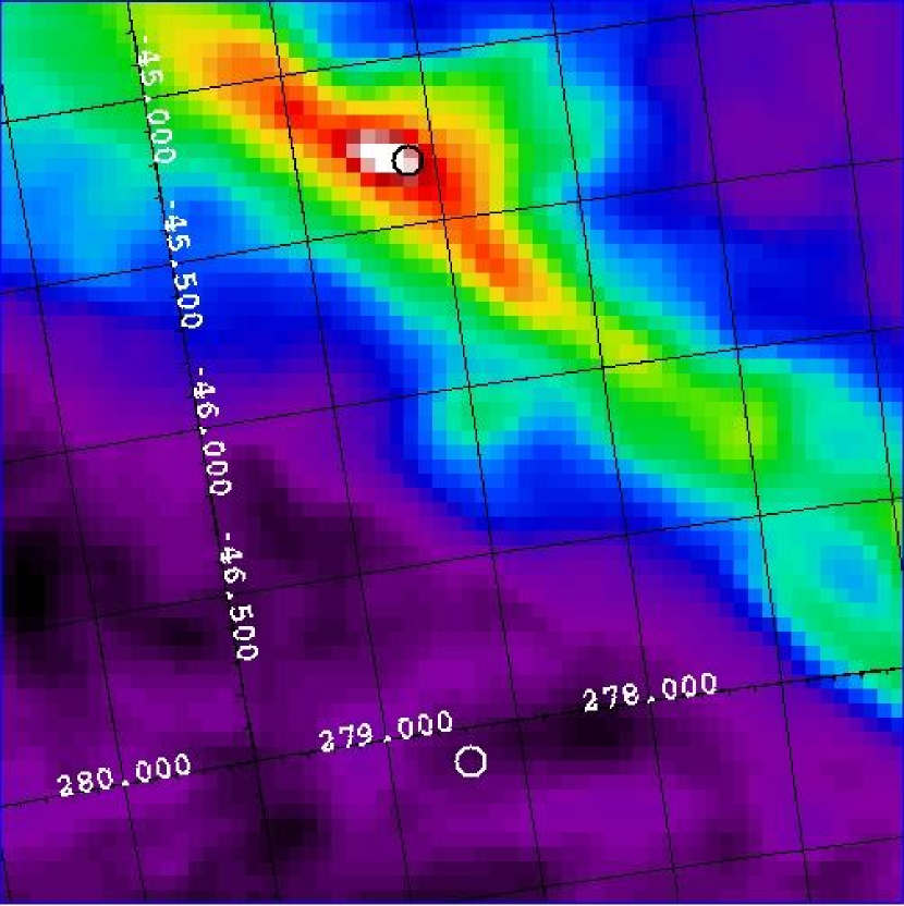
Figure 1: The shadowing filament and nearby sky are shown in this infrared map made from DIRBE corrected IRAS 100 $\mu$m data. The filament runs diagonally across the upper right portion of the image. During the “shadowed” observation, FUSE was pointed toward the most opaque portion of the filament ($278.6^{\rm{o}},-45.3^{\rm{o}}$, within the upper circle). During the “unshadowed” observation, FUSE was pointed toward a low opacity region just off of the filament ($278.7^{\rm{o}},-47.1^{\rm{o}}$, within the lower circle). The FUSE   LWRS aperture measures $30^{\prime\prime}\times 30^{\prime\prime}$, thus a small fraction of the size of the overlayed circles.

For our shadowed line of sight, we used the strength of O VI emission found along the path to a nearby, opaque filament. The filament is located $230\pm 30$ pc from the Sun (Penprase et al., 1998), so is positioned beyond, but not far beyond the Local Bubble. FUSE  has already observed a dense part of the filament at $l=278.6^{\rm{o}},b=-45.3^{\rm{o}}$. The observation yielded a 2$\sigma$ upper limit on the O VI doublet’s intensity, including the systematic uncertainties, of 800 photons s^-1 cm^-2 sr^-1 (Shelton, 2003). Ignoring the systematic uncertainties and using the $1\sigma$ statistical uncertainties as error bars leads to a best fit value of $30\pm{340}$ photons s^-1 cm^-2 sr^-1 (as determined by one of us (RLS) while preparing the original article). To measure the combined halo and Local Bubble O VI intensity for this paper, we used FUSE to observe an unobscured line of sight only 2^o from the filament ($l=278.7^{\rm{o}},b=-47.1^{\rm{o}}$; see Figure 1). In order to estimate the halo’s soft X-ray count rate, we perform a similar shadowing analysis using ROSAT data for the same pointing directions. We also subtract the extragalactic soft X-ray contribution and account for the variation in optical depth with photon energy. By carefully isolating the halo emission, we expect to circumvent the amalgamation problem seen in plots of total O VI intensity versus total soft X-ray countrate.

In Section 2 of this paper we present our measurements of the O VI emission produced along the unobscured, off-filament line of sight. In Subsection 2.4, we subtract the local O VI intensity from our measurement of the unobscured line of sight, yielding the intensity originating in the halo. We determine the halo’s O VI column density from published data for nearby directions in Subsection 2.5. In Subsection 2.6, we estimate of the halo’s 1/4 keV surface brightness by performing a shadowing analysis with ROSAT data from the filament and off-filament directions. We then use the halo’s O VI intensity and column density determinations and treat the O VI-rich gas as if it is isothermal in order to estimate the density and pressure of the emitting material in Subsection 3.2. We compare the O VI and 1/4 keV results with simulation predictions in order to estimate the plasma’s maturity in Subsections 3.4. We compare the O VI and 1/4 keV results with analytic functions in order to estimate the plasma’s temperature distribution function, pressure, and cooling rate in Subsection 3.5. The results are summarized in Section 4.

2 Observations, Data Reduction, Spectral Analysis, and Determination of the Halo’s O VI Intensity

2.1 Observations

FUSE observed the blank sky toward $l=278.69^{\rm{o}},b=-47.08^{\rm{o}}$ (R.A. = $03^{\rm{h}}20^{\rm{m}}10^{\rm{s}}$, decl. = $-62^{\rm{o}}26^{\prime}29^{\prime\prime}$) once in July and twice in November of 2002, for Guest Observer program C153. These observations exposed the LiF 1A detector segment, the segment used for the subsequent O VI signal extraction, for 53, 104, and 61 ksec, respectively. Of these durations, 6, 61, and 26 ksec, respectively, occurred while the satellite was in the night portion of its orbit. FUSE also made a non-proprietary “Early Release Observation” of this direction in December 1999 and archived the data under program identification number X0270301. However, detector 1 was de-powered during most of the observation time.

2.2 Data Reduction

During most of the Guest Observer exposures, data were taken on all four detector segments (1A, 1B, 2A, and 2B). The data from each detector segment were taken in time-tag mode where the photoevents from each detector are listed in the sequence that they were recorded, with their times and locations on the detectors where they were found. We concatenated the photon lists obtained from the individual exposures, creating lists for each detector segment and observation.

We then ran the concatenated photon lists through version 3.1.1 of the CalFUSE pipeline (Sahnow et al., 2000; Dixon, Kruk & Murphy, 2002), with corrections enabling us to use the extended source extraction window. We did not use automatic background subtraction. For the LiF 1A extractions, we set the lower and upper pulse height limits to 4 and 25, respectively. For the other detector segments, we used the default pulse height limits. This process yielded several spectra, because in addition to recording emission with four detector segments, FUSE records light reflected off of each of two types of coatings (lithium fluoride (henceforth called LiF) and silicon carbide (henceforth called SiC)) and four gratings. The multiplicity enables the telescope to see eight overlapping wavelength regimes with various efficiencies. Furthermore, each mirror’s focal plane assembly has four apertures. Thus, each detector segment is able to receive light from each of the four apertures simultaneously and without overlap. The spectra observed through the largest aperture (LWRS: 30” $\times$ 30”) in the LiF1A channel provides the greatest signal to noise and the greatest effective area in the 1030 to 1040 Å regime. We will use these spectra for the following O VI data reduction, and will use the spectra from the other channels when searching for other cosmic emission lines outside of the 1030 to 1040 Å bandpass. Our avoidance of the SiC channels overcomes the solar O VI line contamination problem discussed by Lecavelier des Etangs et al. (2004).

The wavelength scales for each spectrum require re-calibration, which we determined by comparing the reported heliocentric wavelengths of the observed geocoronal emission lines around 1027 and 1040 Å with their rest wavelengths (Morton, 1991) converted from the geocentric to the heliocentric reference frame. We fit a linear function of wavelength to the difference between the expected and observed heliocentric wavelengths, then subtracted this function from the observed wavelengths. We then combined like spectra and shifted to the Local Standard of Rest (LSR) reference frame.

2.3 Spectral Analysis

Figure 2 displays the satellite-night and day$+$night LiF 1A spectra for wavelengths between 1027 and 1045 Å. The spectra reveal O VI emission in the 1032 and 1038 Å lines (rest wavelengths: 1031.93 and 1037.62 Å) and C II^∗ emission at 1037 Å (rest wavelength: 1037.02 Å). An additional emission feature appears in the day+night spectrum at 1031 Å, but does not appear in the night-only spectrum. It also appears in other long-duration FUSE daytime spectra but not in their nighttime counterparts. We suspect that the 1031 Å feature is the second order diffraction peak associated with atmospheric He I, whose rest wavelength is 515.62 Å. Other He I second order lines in our bandpass include $2\times 522.21$ Å and $2\times 537.03$ Å, both of which appear in our daytime spectrum but not our nighttime spectrum. Along with the emission lines is also a continuum, which arises from radioactive decay within the detector, high energy particles, and scattered terrestrial airglow photons. The last of these is strongest during the daytime portion of the orbit.

We used two methods to measure the strengths of the interstellar emission features. With the first method, which parallels that of Shelton et al (2001), we fit a second order polynomial to the continuum of the counts spectrum. (Note that “counts” are called “weights” in CALFUSE version 3.1 output files.) We then subtracted the continuum from the spectrum and searched for wavelength regions with large numbers of counts. Due to continuum subtraction and statistical variation, a few of the pixels within weak emission features have negative numbers of counts and some pixels outside of the emission features have positive numbers of counts. Although this noise complicated our effort to determine the boundaries of emission features, we set the boundaries of the emission features so as to exclude neighboring regions exhibiting near random fluctuations. We then summed the residual counts in each emission feature, divided by the instrumental effective area, and incorporated geometric factors in order to convert the measurements to units of intensity. Each measurement’s statistical uncertainty was calculated from the square root of the number of counts in the original spectra between the upper and lower wavelength range of the feature.

In the day$+$night spectrum, the O VI 1032 Å emission line and the daytime 1031 Å feature are too close together to be separated with this algorithm. Therefore, when we analyzed the 1032 Å emission line in the day$+$night data, we used the wavelength range found from the nighttime data (1031.64 Å to 1032.45 Å). As can be seen in Figure 2, the lower end of this range overlaps very little with the He I feature. Furthermore, the measured intensity in the day$+$night 1032 Å O VI feature is less than that of the night time feature, leading us to believe that little or no He I emission was attributed to the day$+$night 1032 Å feature. Table 1 lists the measured intensities and 1 sigma statistical uncertainties of the O VI 1032 and 1038 Å lines, the C II^∗ line, and the anomalous 1031 Å feature. For presentation purposes, we round the intensities as well as the Local Bubble intensity in §2.4 to 10s of photons sec ^-1 cm^-2 sr^-1. We use the unrounded values when calculating resulting quantities. Given the uncertainties in aperture size and flux calibrations, additional systematic uncertainties of $14\%$ are expected (Shelton et al, 2001). Placement of the continuum is another source of uncertainty. Since the continuum was independently determined during each analysis, the variation within our set of measurements provides an estimate of the size of this uncertainty. The standard deviation among the 4 measurements of the 1032 Å emission line (Table 1) is 220 photons s^-1 cm^-2 sr^-1 while the standard deviation for the 1038 Å line is 470 photons s^-1 cm^-2 sr^-1.

In order to determine the central wavelengths of our irregular, weak emission features, we fit each residual spectrum with a Gaussian and a quadratic. Generally, the fitting routine modeled the emission line with the Gaussian and the residual background with the quadratic. Occasionally, as occurred in the O VI 1032 Å fits, the Gaussian extended beyond the bulk of the emission line in order to include nearby weak residual background emission. Thus, the reported wavelengths for the day$+$night O VI 1032 Å Gaussian fit and the nighttime O VI 1038 Å Gaussian fit are higher and lower, respectively, than one would estimate by eye. See Table 2 for the tabulated results and note that the corrected FUSE scale is accurate to only $\sim 10$ km sec^-1.

In the second method, which parallels that of Dixon et al. (2001), we fit the intensity spectrum’s continuum with a straight line and its emission features with Gaussian shapes that had been convolved with a 106 km sec^-1 top-hat function (simulating the finite width of the LWRS aperture). Because the O VI 1032 Å emission line and the daytime 1031 Å  emission feature are so close together in the day$+$night spectrum, they were fit simultaneously. The O VI 1038 Å emission line and the C II^∗ emission line required simultaneous fitting for the same reason. The fits occasionally included outlying emission, which shifted the reported centroid wavelengths and increased the areas under the curves. The $1\sigma$ error bars for each model parameter were determined as described in Dixon et al. (2001). See Tables 1 and 2 for the measured intensities and velocities.

The O VI and C II^∗ appear to be moving very slowly relative to the Local Standard of Rest. However, the 1032 Å signal is offset by about 30 km s^-1 from the 1038 Å signal, even in the fits that were not corrupted by outlying emission, the night-only 1032 Å and the day+night 1038 Å fits. The difference may be due to inaccuracies in the wavelength scale, being as the observed difference is somewhat more than twice the uncertainty in the velocity of each feature. It could also be due to variations in self-absorption optical depth as a function of wavelength. Larger differences have been seen in other spectra, for example the Virgo and Coma spectra of Dixon et al. (2001). In the night-only 1032 Å and the day+night 1038 Å fits, the $\sigma$ of the cosmic emission lines’ Gaussian profiles were 47 and 39 km s^-1, respectively. The resulting full widths at half maximum are 111 and 92 km s^-1, respectively, while the Doppler parameters are 65 and 55 km s^-1, respectively. The true widths of the cosmic emission lines should be slightly narrower than these values because the fitting method accounts for only the broadening due to a finite slit width and not any other form of instrumental broadening.

As a result of applying two analysis methods to two dataset variants (the day $+$ night data and the night only data), we have 4 measurements for each of the O VI 1032 Å, O VI 1038 Å, and C II^∗ 1037 Å emission lines. For the most part, the $1\sigma$ measurements overlap. However, for each cosmic line, 3 of the 4 intensity measurements are similar to each other while the 4th measurement is an outlier. From the 3 clustered and unrounded measurements, we calculate average intensities of the O VI 1032 Å line, 1038 Å line, and the C II^∗ line. They are 3190$\pm$450$,1520\pm$350, and 1600$\pm$330 photons sec^-1 cm^-2 sr^-1, respectively.

Our O VI signals are neither especially bright nor especially dim when compared with the mid latitude ($35\arcdeg\leq b\leq 60\arcdeg$) FUSE detections in the Otte & Dixon (2006) and Dixon et al. (2006) survey. The larger of these compilations, that of Dixon et al. (2006), lists 17 sight lines having 2 $\sigma$ and 3 $\sigma$ detections of moderate velocity (-100 km s^-1 $\leq v\leq$ 100 km s^-1) O VI 1032 Å emission. Of these 17 signals, 10 were brighter and 7 were dimmer than our 1032 Å signal.

We also examined the data for signs of other cosmic emission lines. No significant signals were found. Our search for C III emission at 977.02 Å in the satellite-night SiC 1B spectrum yielded an intensity $\pm 1\sigma$ of 1300 $\pm$ 1740 photons sec^-1 cm^-2 sr^-1. Similarly, our search for N II emission at 916.71 Å in the same spectrum yielded 510 $\pm$ 1250 photons sec^-1 cm^-2 sr^-1. Although neither species is observed in our dataset, both are observed at the $\geq 2\sigma$ level in the on-filament observation (C III: 4700 $\pm$ 1300 and 2600 $\pm$ 1000 photons sec^-1 cm^-2 sr^-1 in the nighttime SiC 1B and SiC 2A spectra, respectively; N II: 2300 $\pm$ 1100 photons sec^-1 cm^-2 sr^-1 in the night time SiC 1B spectrum, Shelton (2003)). Perhaps the observed photons came from the filament itself. Though, if this is the case, then the C III intensity is remarkably bright, considering that theoretical predictions for evaporating clouds (Slavin, 1989), predict an order of magnitude dimmer emission.

2.4 Determination of the O VI Intensity from the Halo

Along our line of sight, the combined intensity arising from both members of the O VI doublet is 4710 $\pm$ 570 photons cm^-2 s^-1 sr^-1. The observed intensity can be apportioned between the Local Bubble (plus heliospheric) and ‘halo’ components if we assume that the local emission is approximately constant over small angular separations. The observation of an opaque filament on a nearby direction, $\ell=278.6^{\rm{o}},b=-45.3^{\rm{o}}$, set upper limits on the local O VI intensity (Shelton, 2003). For the local contribution, we take the tightest 1 $\sigma$ upper limit (due to random variation only) on the doublet from the day$+$night data for the 1032 Å emission line and the assumption that the 1038 Å line is half as strong as the 1032 Å line. This doublet intensity is $30\pm{340}$ photons cm^-2 s^-1 sr^-1. However, since the Local Bubble cannot produce negative photons, we adjust the estimated intensity arising within 230 $\pm$ 30 pc of the Earth (thus within 160 $\pm$ 20 pc of the Galactic plane) to $30^{+340}_{-30}$ photons cm^-2 s^-1 sr^-1. Thus, for our sight line, the remainder and vast majority of the observed intensity ($4680^{+570}_{-660}$ photons cm^-2 s^-1 sr^-1) is produced in the halo.

Note that the filament data were later included in the Dixon et al. (2006) catalog. To understand the Dixon et al. (2006) reanalysis, the reader needs to first know that the filament was observed in 5 sets of grouped LWRS exposures, taken over a 2 year period, towards 3 very similar directions on the sky (($\ell=278.58^{\rm{o}},b=-45.31^{\rm{o}}$), ($\ell=278.59^{\rm{o}},b=-45.30^{\rm{o}}$), and ($\ell=278.63^{\rm{o}},b=-45.31^{\rm{o}}$)). Figure 3 of Shelton (2003) shows that all three directions point toward a dense knot in an infrared-bright filament. Shelton (2003) separately plotted the spectra for each of the three directions, found no important systematic differences between the spectra, then added the spectra and searched for emission in the O VI 1032 and 1038 Å lines. No emission was found near the Milky Way’s Local Standard of Rest (LSR) velocity in either line, in either the data taken during the satellite night portion of the orbit or data taken during the the satellite day + night portions of the orbit. In our shadowing analysis (previous paragraph), we have adopted the tightest $1\sigma$ upper limit for the doublet, excluding systematic uncertainties, from the Shelton (2003) analysis. It was derived from the day+night data for the O VI 1032 Å region.

The later analysis by Dixon et al. (2006) differed from that of Shelton (2003) because it included only data taken during orbital night, searched for only the 1032 Å emission line, and used a different version of the pipeline, different choices of pulse height cutoffs, and a different spectral fitting algorithm. They noticed a high velocity feature in their combined dataset, but determined that it was primarily associated with their data taken towards $\ell=278.59^{\rm{o}},b=-45.30^{\rm{o}}$. In that direction, their O VI 1032 Å feature’s velocity and intensity are $206\pm 13$ km s^-1, and $3.0\pm 0.6\times 10^{3}$ photons cm^-2 s^-1 sr^-1, respectively. In contrast, neither of their spectra in the other directions revealed statistically significant O VI 1032 Å emission. From this, Dixon et al. (2006) concluded that O VI in the Magellanic Stream moving at $\sim 200$ km s^-1 relative to the LSR had been viewed through a previously unknown hole in the filament and that the other observations viewed opaque portions of the filament. When Dixon et al. (2006) excluded the red-shifted feature from their analysis of the combined dataset, they derived a $2\sigma$ upper limit on the O VI 1032 Å emission of $600$ photons cm^-2 s^-1 sr^-1 (see the last paragraph of their Appendix A.2 and note that their naming convention differs from that of Shelton (2003)), which is roughly similar to the $2\sigma$ upper limit reported by Shelton (2003). Given that they did not find LSR rest frame emission, they did not modify the conclusions of Shelton (2003) regarding the physical conditions in the Local Bubble.

If the high velocity O VI reported by Dixon et al. (2006) were to lie along the off-filament line of sight analyzed in this paper, then its 1032 Å emission would be $90\%$ as bright as and 0.6 Å longwards of the O VI 1032 Å feature we observed. As can be seen in Fig. 2, our spectra are dim around $\lambda=1032.64$ Å, the wavelength of O VI traveling at 206 km s^-1. Our wavelength calibration in this part of the spectrum is good to within $\sim$0.034 Å ($\sim$10 km s^-1); therefore, the observed velocity of the O VI 1032 Å feature in our spectrum is inconsistent with the reported velocity of the Dixon et al. (2006) feature. Thus, we conclude that the high velocity, presumably extra-galactic feature seen by Dixon et al. (2006) in the I2050501 + I2050510 data has not appeared in the off-filament data and does not affect our analysis of the halo’s emission.

Next we consider the effects of extinction. Our off-filament line of sight is only mildly extincted, but we obtain somewhat different results from different datasets. According to the DIRBE and IRAS data (Schlegel, Finkbeiner, & Davis, 1998), its color excess is E(B-V) = 0.0217, implying that $N({\rm H~{}I})=1.06\times 10^{20}{\rm cm}^{-2}$ if we use the empirical relation $N({\rm H~{}I})/E(B-V)=4.93\times 10^{21}{\rm cm}^{-2}$ derived by Diplas & Savage (1994). Thus, we expect that 25$\%$ of the photons originating beyond the obscuring material have been extincted (Fitzpatrick, 1999). However, according to the Leiden-Argentine-Bonn Survey (Kalberla et al, 2005), the column density of neutral hydrogen, $N_{\rm HI}$, is $2.04\times 10^{20}$ cm^-2 on the two nearest lines of sight ($(l,b)=278.69,-47.08$ and $278.80,-47.00$), equating to a color excess of 0.0414 (Diplas & Savage, 1994) and an extinction loss of $42\%$ (Fitzpatrick, 1999). We recognize that this may slightly overestimate the amount of hydrogen along our line of sight because some small portion of the $0\fdg 6$ (HPBW) diameter beam could be responding to the emission from the filament. We will take $N_{\rm HI}=2.0\times 10^{20}$ cm^-2 as the upper end of the possible range.

For a lower limit to the absorption, we consider the extreme case that a large fraction of the neutral hydrogen might be beyond the O VI-emitting gas (almost all of which must be more distant than the shadowing filament). A limit to that fraction is defined by an estimate for the amount of H I that exists within the Local Bubble. Lallement et al. (2003) found that well in front of the distance to the filament (230 $\pm$ 30 pc) the equivalent widths of intervening Na I D absorption in the spectra of stars in the general vicinity of our sight line are at least 20 mÅ and perhaps even as large as 50 mÅ (corresponding to $N_{\rm HI}=0.5$ to $2.0\times 10^{20}$ cm^-2, respectively.) Thus, there must be some extinction between our location and the O VI ions. Allowing for small scale variations in ISM column densities and for possible revisions in the distance estimates, we take $N_{\rm HI}=0.5\times 10^{20}$ cm^-2 as our lower limit. Also, we take $N_{\rm HI}=1.0\times 10^{20}$ cm^-2 as our nominal value. For $N_{\rm HI}=1.0\times 10^{20}$ cm^-2, the intrinsic intensity, $I_{\rm OVI}$, is $6110^{+740}_{-860}$ ($11.8^{+1.4}_{-1.7}\times 10^{-8}$ erg cm^-2 s^-1 sr^-1). For the extreme range of possible extincting column densities, $N_{\rm HI}=0.5$ to $2.0\times 10^{20}$ cm^-2, the intrinsic intensity, $I_{\rm OVI}$, is $5350^{+650}_{-750}$ photons cm^-2 s^-1 sr^-1 ($10.3^{+1.2}_{-1.5}\times 10^{-8}$ erg cm^-2 s^-1 sr^-1) to $7960^{+970}_{-1120}$ photons cm^-2 s^-1 sr^-1 ($15.3^{+1.9}_{-2.2}\times 10^{-8}$ erg cm^-2 s^-1 sr^-1).

2.5 An Estimate for the Halo’s O VI Column Density

In order to determine a characteristic electron density for the hot gas, we must know the halo’s O VI column density ($N_{\rm OVI}$). To estimate $N_{\rm OVI}$ along our line of sight, we have at our disposal only determinations made in other directions about $15\arcdeg$ away (Wakker et al, 2003). We make use of 4 such measurements and evaluate their average column density. This average equals $2.34\times 10^{14}$ cm^-2 towards (1) NGC 1705, (2) Fairall 9, (3) several targets within the LMC, which we treat as a single data point, and (4) several targets within the SMC, which we also treat as a single data point (Savage et al., 2003). While this mean value represents our best estimate for our direction, we recognize that O VI column densities vary markedly over angular separations of $15\arcdeg$, and thus our adopted value could deviate substantially from the true value.

We now estimate the size of the error in our determination. By examining Figure 11 of Savage et al. (2003), we can better estimate the expected deviation from the parent population than simply evaluating the internal dispersion of the nearest 4 lines of sight considered here. The average difference in column density of individual sight lines in pairs with $\sim 15\arcdeg$ separations in the data set of Savage et al. (2003) is $35\%$ of the mean of each pair. Thus, on average, each determination differs from the mean of the two by $17.5\%$. The root-mean-square ($rms$) deviations should be $\sqrt{\pi/2}$ times this value if the distribution is Gaussian, and individual samples drawn from the parent population have dispersions that are a factor of $\sqrt{2}$ larger, leading to a fundamental $rms$ deviation of $31\%$ from what we could consider to be a “true” overall mean value over some arbitrarily large sector of the sky. The mean of 4 randomly drawn samples from the parent population should deviate from the overall mean by only half as much ($15.5\%$). Thus, our estimate for $N_{\rm OVI}$ along our line of sight based on the other 4 measurements could be in error by an amount equal to the error in the mean ($15.5\%$) combined in quadrature with the intrinsic fluctuations in the individual lines of sight ($31\%$), giving a total uncertainty of $34.7\%$. Thus, we estimate the O VI column density and 1 $\sigma$ error for our line of sight should equal $2.34\pm 0.81\times 10^{14}$ cm^-2.

From this value, we must subtract the Local Bubble’s column density, which we estimate from its O VI volume density and radius. Three of the white dwarfs in the Savage & Lehner (2006) survey of nearby stars are within 30^o of our pointing direction. The volume densities on these short and nearby lines of sight range from $2.01$ to $10.6\times 10^{-8}$ O VI ions cm^-3. From Figure 6 in Lallement et al. (2003), we take the radius of the Local Bubble in our direction to be 80 to 140 pc. From the minimum radius and O VI volume density, we estimate the minimum Local Bubble O VI column density to be $5.0\times 10^{12}$ cm^-2, and from the maximum radius and O VI volume density, we estimate it to be $4.58\times 10^{13}$ cm^-2. Conservatively adopting these values as the Local Bubble’s average column density $\pm$ 1 $\sigma$ and subtracting them from the column density toward extragalactic targets yields the halo column density, $N_{\rm OVI}=2.09\pm 0.84\times 10^{14}$ cm^-2

2.6 An Estimate for the Halo’s X-Ray Brightness

We now use results from the ROSAT All Sky Survey to find X-ray intensities that apply to our two lines of sight. We extract the 1/4 keV X-ray count rate from the survey data for the R1 and R2 bands ($\sim 110$ to 284 eV and $\sim 140$ to 284 eV, respectively). A 0.4^o radius disk centered on our direction $l=278.7^{\rm{o}},b=-47.1^{\rm{o}}$, has a combined ROSAT R1 $+$ R2 countrate of 1322 $\pm$ 55 $\times 10^{-6}$ (Snowden et al. (1997), retrieved with the X-Ray Background Tool: http://heasarc.gsfc.nasa.gov/cgi-bin/Tools/xraybf/xraybg.pl). This countrate includes contributions from the halo, Local Bubble, heliospheric charge exchange, and extragalactic objects. Assuming that the Local Bubble contribution is roughly uniform over small angular scales and that the heliospheric contribution is roughly time invariant, we take the Local Bubble plus heliospheric contributions to equal the countrate seen toward the nearby filament (534 $\pm$ 131 $\times 10^{-6}$ counts s^-1 arcmin^-2 for a 0.1^o disk centered on $l=278.6^{\rm{o}},b=-45.3^{\rm{o}}$). In order to estimate the extragalactic contribution, we draw upon the parameterizations of Miyaji et al. (1998). They found that $I(E)=10.0\pm 0.5\times E^{-1.42\pm 0.03}$ and $I(E)=11.5\pm 0.7\times E^{-1.42\pm 0.03}$ photons cm^-2 k^-1 keV^-1 sr^-1 for photon energies, $E$, between 0.1 and 10 keV for the two fields they studied. We take the average: $I(E)=10.75\times E^{-1.42}$ photons cm^-2 k^-1 keV^-1 sr^-1. When absorbed by galactic material (here we take the total column to be as high as $N_{\rm{HI}}=2.0\times 10^{20}$ cm^-2) and convolved with the ROSAT response function, such a spectrum yields 55.6 $\times 10^{-6}$ counts s^-1 arcmin^-2 in the R1$+$R2 bandpass, hereafter termed the R12 bandpass. Subtracting the local and extragalactic contributions from the observed countrate along our line of sight yields a halo countrate of 732 $\pm$ 142 $\times 10^{-6}$ counts s^-1 arcmin^-2. This rate applies if emission originates below all of the observed neutral hydrogen. However, we believe that the halo emission originates above an absorbing column of 0.5 to $2.0\times 10^{20}$ cm^-2. In this case, the intrinsic countrate would be $779\pm 151$ to $4770\pm 930$ counts s^-1 arcmin^-2.

For the analysis that will be presented in § 3.5, we will also require the halo’s R6 + R7 band (hereafter termed the R67 band) countrate. The filament is too optically thin at 1.5 keV for a useful shadowing analysis. However, Henley, Shelton & Kuntz (2006) have performed spectral fits with the ROSAT and XMM data for the on-filament and off-filament directions. Their analysis takes into account the extragalactic and Local Bubble contributions, as well as instrumental and other sources of noise. According to David Henley (personal communication), the halo’s intrinsic intensity in the R67 band is $\sim 30$ counts s^-1 arcmin^-2.

3 Discussion

3.1 The Heavy Element Abundances

Many of the calculations performed in this paper are dependent, to varying degrees, on the assumed abundance ratios of heavy elements to hydrogen, since we reported on observations of atomic transitions of either oxygen (in the case of O VI emission or absorption) or an ensemble that includes many other heavy elements (the main source of soft x-ray emission). Beyond an application to our observations, heavy element abundances also influence some theoretical aspects of our subject matter, such as all processes that depend the rate of radiative cooling of the gas. While we recognize that the abundances can vary with galactocentric distance (Peimbert, 1999; Martín-Hernández et al, 2002; Daflon & Cunha, 2004; Esteban et al, 2005), and even from one place to the next at a given radius from the center (Edvardsson et al, 1993; Rolleston, Dufton & Fitzsimmons, 1993), we adopt the simplest interpretation that the abundances agree with the solar values. Even here, however, there are choices to be made. While the outcomes for determinations of the solar abundances of elements heavier than oxygen have been reasonably stable through the years (Grevesse & Sauval, 1998), very recently there have been some substantial downward revisions for C, N and O, based on interpretations of line strengths in the context of detailed models of line formation in a convective atmosphere (Holweger, 2001; Allende Prieto, Lambert, & Asplund, 2002; Asplund et al., 2004). Of particular relevance to our work is the change in the solar abundance of oxygen relative to hydrogen, which has recently declined by 0.27 dex. While there has been some independent support for the new oxygen abundance, based on abundances found for O- and B-type stars (Daflon et al, 2003), it is discordant with models of the sound speed inside the Sun and the depth of its convective zone, based on the interpretations of helioseismological data (Bahcall & Serenelli, 2004; Bahcall et al, 2004; Antia & Basu, 2005) coupled with models that incorporated more accurate calculations of atomic opacities (Badnell et al., 2005). The problem might be solved with a higher abundance of Ne to compensate for the decreased abundances of C, N and O (Antia & Basu, 2005; Drake & Testa, 2005; Cunha et al, 2006), but this proposal has been met with some skepticism (Asplund et al., 2005). In view of the fact the solar abundance of oxygen might still be questioned, in various sections of this paper we will discuss the consequences of adopting either the old or new values. In cases where we make our own calculations, we favor the new abundances, but our use of some older, relatively complex models discussed in §3.4 and §3.5 were based on the old abundances.

3.2 The Physical Properties of O VI-bearing Gas (Isothermal Case)

To introduce the basic concepts of our analysis of some relevant physical parameters, we start with the simplest case where the hot gas is isothermal and at the temperature that corresponds to that where O VI has its maximum ion fraction when the gas is in CIE ($3.2\times 10^{5}$ K). The density of electrons ($n_{e}$) in the plasma that bears the O VI ions can be calculated from the halo’s O VI column density derived in §2.5, intrinsic doublet intensity derived in §2.4, and temperature ($T$, assumed to be the CIE temperature, $3.2\times 10^{5}$ K, but the calculation is relatively insensitive to temperature if $10^{5}$ K $>T>10^{6}$ K). We use Equation 5 in Shull & Slavin (1994): $n_{e}=(4\pi I_{\rm OVI})/(<\sigma\nu>_{e}N_{\rm OVI})$, where $<\sigma\nu>_{e}$ is the electron-impact excitation rate coefficient. If the observed emission originates beyond an extincting column of $N_{\rm HI}=1.0\times 10^{20}$ cm^-2, then $n_{e}=12.5^{+5.2}_{-5.3}\times 10^{-3}$ cm^-3, but if it lies beyond our extreme estimates, $N_{\rm HI}=0.5$ or $2.5\times 10^{20}$ cm^-2, respectively, then $n_{e}=11.0^{+4.6}_{-4.7}$ or $n_{e}=16.3^{+6.8}_{-6.9}\times 10^{-3}$ cm^-3 (see Table 3.)

Table 3 also lists the thermal pressure and the depth of the emission region. The thermal pressure, $p_{th}$, is calculated from the ideal gas law. Taking the cosmic abundance of the elements into account results in $p_{th}/k=1.92n_{e}T$. The depth of the emitting region, $\Delta l$, is equal to the column density of O VI divided by the product of the electron density and three calculated ratios: (H/$e$), which equals 0.833 in a fully-ionized plasma with a cosmic composition, $({\rm O/H})_{\odot}$, for which we adopt a value $4.57\times 10^{-4}$ given by Asplund et al. (2004), and the peak value of the fractional ion concentration arising from the balance of collisional ionizations and various recombination processes, $f_{\rm O~{}VI}(T_{\rm max})$, calculated by Nahar & Pradhan (2003). Our result for $\Delta l=N_{\rm{OVI}}/\{n_{e}\times({\rm{H}}/$e$)\times({\rm O/H})_{\odot}\times f_{\rm O~{}VI}(T_{\rm max})\}$ is nearly a factor of 2 larger than that presented in previous papers (i.e. Shelton et al (2001)), because the oxygen abundance estimates of Asplund et al. (2004) are nearly a factor of 2 smaller than those of Grevesse & Anders (1989). Lastly, we calculate the time required for the gas to cool, if it were to cool solely by the emission of O VI resonance line photons. (See Table 3.) The timescale estimates are inversely proportional to the oxygen abundance. The quoted estimates are approximately twice as large as they would have been if we had used the Grevesse & Anders (1989) oxygen to hydrogen ratio. Furthermore, the quoted timescales are upper limits on the true cooling timescales for the present O VI-rich gas and do not include cooling of nearby, hotter gas that may, in the future, evolve through an O VI-rich stage. In the following subsections, we will compare these simple predictions with those of more comprehensive models.

3.3 The Extended Baseline Spectrum

In this subsection, we create a long baseline spectrum from the halo’s O VI and soft X-ray emission. For our comparison between the 1/4 keV and O VI intensities in § 3.4, we must convert the ROSAT R12 countrate to units of intensity. In order to estimate the conversion rate factor, we take the X-ray spectrum as that of a $T=10^{6}$ K, CIE plasma, as determined by Bloch et al. (1986) and Pietz et al. (1998); Kuntz & Snowden (2000) found this temperature to be the dominant temperature component in their analysis of the halo’s soft X-ray emission (the other component is $T=3\times 10^{6}$ K). As a result, the halo’s intensity in $\sim 110$ to 284 eV photons is $2.2\pm 0.4\times 10^{-8}$ ergs s^-1 cm^-2 sr^-1 if the emission originates above $N_{\rm{HI}}=0.5\times 10^{20}$ cm^-2 and $13.4\pm 2.6\times 10^{-8}$ ergs s^-1 cm^-2 sr^-1 if it originates above $N_{\rm{HI}}=2.0\times 10^{20}$ cm^-2. The intensity of the entire 1/4 keV band amounts to only 21$\%$ of the intensity in the O VI doublet if the halo emission originates above extincting material having $N_{\rm{HI}}=0.5\times 10^{20}$ cm^-2 and 87$\%$ of the O VI doublet intensity if the halo emission originates above $N_{\rm{HI}}=2.0\times 10^{20}$ cm^-2. As an aside, it is of interest to compare these numbers with the local (Local Bubble $+$ heliospheric) X-ray to O VI ratio, which is at least 1.4 for the on-filament line of sight. Thus, the local region preferentially sheds energy via the soft X-ray emission lines while the halo preferentially sheds energy via the O VI emission lines. We note that interpreting the relationship between the O VI and X-ray emission rests on the assumption that the same regions of space are being sampled. The OVI and X-ray data are from the same directions, but have differing fields of view and differing optical depths due to the dependence of optical depth on photon energy. As a result, the assumption is not strictly correct. The extent to which this is an issue depends in part on the small scale structure in the ISM, but is anticipated to affect our results less than the other simplifications involved in our modeling.

Although a collisional ionizational equilibrium spectrum at $T=10^{6}$ K has been found to fit the soft X-ray data, it underpredicts the O VI intensity (even when we assume that the halo emission has been absorbed by $N_{\rm{HI}}=2.0\times 10^{20}$ cm^-2.) As the model’s temperature is lowered, its soft X-ray emission decreases more rapidly than its O VI emission. Therefore, it is possible to find a single temperature spectrum that matches both the halo’s O VI and the 1/4 keV intensities. However, the assumed temperature is significantly less than $10^{6}$ K, and so does not produce the soft X-ray band ratios observed across much of the high latitude sky. Therefore, we will move on to more complex models which are inspired by physically conceivable events.

3.4 The Expected Outcome for a Halo Supernova Remnant

We now examine the expected consequences for a line of sight in the halo that is dominated by the effects of a single SN event. Our rationale is that in most explanations for the hot halo gas, the gas had been heated suddenly by an energetic event in the past. Irrespective of whether the energetic events occurred above the Galactic disk (i.e. extraplanar supernova explosions and collisions between infalling clouds and the Milky Way) or in the disk and the hot gas later rose into the halo, we expect the plasma to evolve from a recently shock heated and underionized state to a tepid and overionized state; and we expect the observationally determined O VI to soft X-ray ratio to be a useful diagnostic. In the following halo SNR simulations, we found that the ratio of O VI to 1/4 keV emission rises almost monotonically throughout the remnant’s life, making it a diagnostic of the remnant’s maturity.

We calculated the ratio of O VI to ROSAT 1/4 keV intensities from a simulated, extraplanar supernova remnant. For the simulation, we set the ambient density, explosion energy, and ambient nonthermal pressure to 0.01 atoms cm^-3, $0.5\times 10^{51}$ ergs, and 1800 K cm^-3, respectively. As in Shelton (1999), the simulation included thermal conduction and non-CIE radiative cooling. The ionization and recombination rates were calculated using the Gaetz, Edgar, & Chevalier (1988) tables and the spectra were calculated from the plasma’s non equilibrium ionization level populations and the Raymond & Smith (1977) algorithm. We used the Grevesse & Anders (1989) abundance tables, in which the oxygen to hydrogen ratio is approximately a factor of 2 greater then that found by Asplund et al. (2004). The predicted O VI intensity roughly scales with the adopted oxygen abundance, while the 1/4 keV soft X-ray spectrum is mostly unaffected.

Here, we describe the plasma’s evolution and the consequent O VI to X-ray ratio’s evolution. When the halo supernova remnant is very young (age $<$ 10,000 yrs), its most emissive portion is the hot, dense gas immediately behind the shock front. Due to the rapid ionizations, the recently shock-heated gas in this zone contains O VI and higher ions. Although this plasma emits both O VI resonance line and soft X-ray photons, its temperature ($T>10^{7}$ K) is far too high for optimum O VI resonance line emission. As a result, the ratio of O VI to soft X-ray intensities is less than the observed ratio (see Figure 3). As time passes, the shock front slows, thus heating the gas in and just behind the shock to lesser temperatures and leading to a slight increase in the O VI to X-ray ratio.

Before the remnant is $\sim 50,000$ years old, both the hot dense gas near the shock front and the hot rarefied gas in its interior are drastically out of CIE. When the remnant is between 50,000 and 100,000 years old, most of its plasma comes into CIE, but not in the usual manner. Rather than maturing sufficiently for its ionization levels to come into equilibrium with the gas temperature, the gas temperature drops sufficiently as to match the ionization levels (see Figure 4 of Shelton (1999)). At this time, the most important gas, that immediately behind the shock, is close to, but not yet in CIE. During or just before this era, the simulation’s O VI to 1/4 keV ratio crosses that of the observed ratio (1.1, assuming that the intrinsic emission had been absorbed by a $2.0\times 10^{20}$ cm^-2 column, to 4.7, assuming that the intrinsic emission had been absorbed by a $0.5\times 10^{20}$ cm^-2 column). These observationally determined ratios are marked on Figure 3 by horizontal dashed and dot-dashed lines which cross the SNR ratio curve when the remnant is $\sim$40,000 and $\sim$70,000 years old, respectively.

As the remnant continues to cool by adiabatic expansion and radiative cooling, its atoms begin to recombine. When the remnant is between 100,000 and 250,000 years, its shock front becomes too cool to produce much O VI or soft X-ray emission. Thus the shock front no longer outshines the bubble’s interior. The remnant’s O VI to ROSAT 1/4 keV ratio, now primarily due to the remnant’s “overionized” interior, rises. Henceforth, recombinations from O VIII to O VII to O VI provide the remnant’s center with O VI ions while reducing its supply of higher, more X-ray emissive, ions. In time, the temperature drops from $T\sim 10^{6}$ K down to $T\sim 10^{5}$ K, causing the soft X-ray emission function to plummet (although the O VI resonance line emission function remains nearly constant.) As a result, the O VI versus 1/4 keV ratio continues to rise. In its final million years, the remnant is tepid ($T=$ several $\times 10^{4}$ K), contains some O VI ions, but few higher ions. Thus it produces an enormous O VI to 1/4 keV ratio, as shown in the plot.

We observe similar trends in simulated supernova remnants having greater ambient densities, ambient nonthermal pressures, and/or explosion energies, though with some variation in the age when the model matches the observational ratio. Assuming that the observed gas can be compared to that in an undisturbed, extraplanar supernova remnant bubble, the time since heating and the lifetime of this gas are on the order of $10^{4}-10^{5}$ and $10^{7}$ years, respectively. The cooling timescale exceeds that calculated directly from the O VI data (Table 3) because the SNR contains a reservoir of hotter, more highly ionized gas that will eventually transition through the O VI level. Assuming that the other possible sources of hot gas behave similarly to simulated halo SNRs, we suggest that the resulting structure is middle aged.

3.5 The Volume Distribution Function of Temperatures

3.5.1 The Basic Assumptions

We move on to a more generalized picture and propose that the hot gas in the halo of our Galaxy is a heterogeneous mixture of regions having plasmas at different temperatures, created possibly by many SN events whose influences on the halo medium have merged together. A convenient characterization of the temperature distribution function over volume can take on the form of a power-law, one that extends from $10^{5}\,$K (above which appreciable amounts of O VI are expected in CIE) to a sharp cutoff at some high temperature $T_{\rm{cut}}$. Within the paradigm that the hot gas is created by supernova shock waves that are produced in the halo or that escape from the disk, the origin of $T_{\rm{cut}}$ can be interpreted to arise from either a generalized limit on the supernova shock velocities or, alternatively, from our recognition that gases with temperatures that are too high may escape very rapidly in the form of a very low density, high velocity wind, which is difficult to detect.

Since all of the observable effects of the hot gas represent line integrals of various physical quantities through the Galactic halo, there is some benefit in our starting with a formulation that describes how the many differential length segments $dl$ within the population of discrete, homogeneous gas regions are distributed over temperature. We do this by specifying a transformation between $dl$ and $d\ln T$,

$$dl = BT^{\beta}d\ln T~{}{\rm for}~{}T<T_{\rm cut}$$ (1)

$$= 0~{}{\rm for}~{}T>T_{\rm cut}~{},$$ (2)

where $B$ is a distance scale factor. In a broad, statistical sense, this distribution function describes how temperatures are weighted according to volume fractions, but it says nothing about the internal electron densities $n_{e}$ within the length segments.

In the development of our interpretation, we impose a simplifying constraint that the Galactic halo is approximately isobaric. We use this universal pressure constraint to tie the electron density to temperature and thermal pressure, i.e., $n_{e}=p_{th}/(1.92kT)$. While we must accept the reality that some pressure variations can exist from one location to another, we can assume that the magnitude of such variations are small compared to the vastly different temperatures that we adopt in our model. Our representative pressure $p_{th}$ is a free parameter that we will determine from the ratio of $I_{\rm OVI}/N_{\rm OVI}$ after we have solved for the power-law coefficient $\beta$ and temperature limit $T_{\rm cut}$.

3.5.2 How the Observations Relate to the Model

The column density of O VI is given by the expression

$$N_{\rm OVI}=\left({{\rm O}\over{\rm H}}\right)_{\odot}\left({{\rm H}\over e}\right)~{}\int f_{\rm OVI}(T)n_{e}dl$$ (3)

where $(\rm O/H)_{\odot}$, $({\rm H}/e)$, and $f_{\rm OVI}(T)$ were first used in §3.2. We can rewrite Eq. 3 in terms of an integral over $\ln T$ of the temperature distribution we adopted,

$$N_{\rm OVI}=\left({{\rm O}\over{\rm H}}\right)_{\odot}\left({{\rm H}\over e}\right)~{}{p_{th}B\over 1.92k}\int_{\ln 10^{5}\rm{K}}^{\ln T_{\rm cut}}f_{\rm OVI}(T)T^{\beta-1}d\ln T$$ (4)

by making a substitution of the terms in Eq. 1 for $dl$, using the relation $n_{e}=p_{th}/(1.92kT)$, and noting that O VI is rare at temperatures below $10^{5}$ K.

We can develop similar equations for the expected strengths of the line radiation from O VI or the intensities of soft X-rays. For the emission from both members of the O VI doublet, we anticipate that

$$I_{\rm OVI}=\int r_{\rm OVI}(T)n_{e}^{2}dl~{},$$ (5)

where the emission rate coefficient $r_{\rm OVI}(T)$ per unit emission measure is given by

$$r_{\rm OVI}(T)=3.09\times 10^{18}\left({{\rm O}\over{\rm H}}\right)_{\odot}\left({{\rm H}\over e}\right)f_{\rm OVI}{<\sigma v>(T)\over 4\pi}~{}{\rm photons~{}cm}^{-2}{\rm s}^{-1}{\rm sr}^{-1}({\rm cm}^{-6}\,{\rm pc})^{-1}~{}.$$ (6)

As we did in §3.2, we adopt an analytical formulation of $<\sigma v>(T)/(4\pi)$ that was specified by Shull & Slavin (1994). Again after substituting the expression in Eq. 1 for $dl$ and $p_{th}/(1.92kT)$ for $n_{e}$ we find that

$$I_{\rm OVI}={p_{th}^{2}B\over(1.92k)^{2}}\int_{\ln 10^{5}\rm{K}}^{\ln T_{cut}}r_{\rm OVI}(T)T^{\beta-2}d\ln T~{}$$ (7)

A similar equation can be expressed for the soft X-ray emission,

$$R_{12}={p_{th}^{2}B\over(1.92k)^{2}}\int_{\ln 10^{5}\rm{K}}^{\ln T_{cut}}r_{12}[N_{\rm HI},T]T^{\beta-2}d\ln T~{},$$ (8)

where $r_{12}[N_{\rm HI},T]$ is the emission rate coefficient as a function of temperature for 0.25 keV X-rays, matched to the responses of the ROSAT bands 1 and 2 and expressed in the units ${\rm counts~{}cm}^{-2}\,{\rm s}^{-1}\,{\rm arcmin}^{-2}({\rm cm}^{-6}\,{\rm pc})^{-1}$ (Snowden et al. 1997). This coefficient includes the effect of an energy-dependent foreground absorption represented by $N_{\rm HI}$.

3.5.3 Evaluation of Parameters

To evaluate the free parameters $\beta$, $T_{\rm cut}$ and $p_{th}/k$, we compare three ratios of observable quantities with their expectations within our formalism. First, we may constrain the value of $\beta$ by matching the observed ratio of $I_{\rm OVI}$ to $R_{12}$ to the expression

$${I_{\rm OVI}\over R_{12}}={\int_{\ln 10^{5}\rm{K}}^{\ln T_{\rm cut}}r_{\rm OVI}(T)T^{\beta-2}d\ln T\over\int_{\ln 10^{5}\rm{K}}^{\ln T_{\rm cut}}r_{12}[N_{\rm HI},T]T^{\beta-2}d\ln T}~{}.$$ (9)

While the result depends on an adopted value of $T_{\rm cut}$, for reasonably high values of this quantity the effect is small. We find that for $I_{\rm OVI}=4680\,{\rm photons~{}cm}^{-2}{\rm s}^{-1}{\rm sr}^{-1}$ and $R_{12}=0.000733\,{\rm counts~{}cm}^{-2}{\rm s}^{-1}{\rm arcmin}^{-2}$ we obtain $I_{\rm OVI}/R_{12}=6.4\times 10^{6}$ (in the same units) with an uncertainty of 24% using the errors stated in §2. The first row of Table 4 lists the derived values of $\beta$ for the best and limiting values of foreground H I absorption. The top row of panels in Fig. 4 shows how $I_{\rm O~{}VI}/R_{12}$ changes with $\beta$ and demonstrates that the dependence on $T_{\rm cut}$ is not important for $\beta<1.5$ and is a small effect for $\beta<2$.

A strong response to $T_{\rm cut}$ arises from the ratio of high energy X-ray emission to the intensity at lower energies, as indicated in the second row of panels in Fig. 4, where we have made use of an equation that is identical in form to Eq. 9 except that it compares the ratio of X-ray emission at 1.5 keV (the sum of intensities recorded in ROSAT Bands 6 and 7) to that at 0.25 keV (the sum in ROSAT Bands 1 and 2),

$${R_{67}\over R_{12}}={\int_{\ln 10^{5}\rm{K}}^{\ln T_{\rm cut}}r_{67}[N_{\rm H~{}I},T]T^{\beta-2}d\ln T\over\int_{\ln 10^{5}\rm{K}}^{\ln T_{\rm cut}}r_{12}[N_{\rm H~{}I},T]T^{\beta-2}d\ln T}~{}$$ (10)

From the observed value of $R_{67}/R_{12}=0.04$ (§2.6), we arrive at values of $\log T_{\rm cut}$ given in the second row of Table 4.

Finally, we solve for $p_{th}/k$ by matching the observed ratio of $I_{\rm OVI}$ to $N_{\rm OVI}$ to the formula

$${I_{\rm OVI}\over N_{\rm OVI}}={p_{th}\over 1.92k}~{}{\int_{\ln 10^{5}\rm{K}}^{\ln T_{\rm cut}}f_{\rm OVI}[<\sigma v>(T)/(4\pi)]T^{\beta-2}d\ln T\over\int_{\ln 10^{5}\rm{K}}^{\ln T_{\rm cut}}f_{\rm OVI}T^{\beta-1}d\ln T}~{}$$ (11)

Values of $p_{th}$, found for $I_{\rm OVI}/N_{\rm OVI}=2.24\times 10^{-11}$ photons s^-1 sr^-1 with an uncertainty of about 50%, are listed in the third row of Table 4. From the flatness of the curves shown in the third row of panels in Fig. 4, the value of $p_{th}$ is not strongly influenced by the choice of $\beta$ (and has virtually no dependence on $T_{\rm cut}$). The dominant uncertainty in $p_{th}$ arises from the expected error in $I_{\rm OVI}/N_{\rm OVI}$.

It is important to check that the computed width for thermal Doppler broadening of O VI in the model does not exceed the observed widths of the actual absorption profiles observed in the Galactic halo. Our expectation is that

$$<v^{2}>={\int n({\rm OVI})<v({\rm OVI})^{2}>dl\over\int n({\rm OVI})dl}={k\over 16m_{\rm p}}~{}{\int_{\ln 10^{5}\rm{K}}^{\ln T_{\rm cut}}f_{\rm OVI}(T)T^{\beta}d\ln T\over\int_{\ln 10^{5}\rm{K}}^{\ln T_{\rm cut}}f_{\rm OVI}(T)T^{\beta-1}d\ln T}~{},$$ (12)

where $m_{\rm p}$ is the mass of a nucleon. For our derived values of $\beta$, we find that the Doppler parameter $b=(2<v^{2}>)^{\text@frac{1}{2}}$ ranges from 19 to $23\,{\rm km~{}s}^{-1}$. These values are smaller than the representative observed values, which are of order $60\,{\rm km~{}s}^{-1}$. Evidently, even with our allowance for some O VI arising from temperatures above $10^{6}\,$K, the expected profile widths are still much less than the kinematic broadening that takes place in the halo. As with our findings on $p_{th}/k$, the bottom row of panels in Fig. 4 shows that the outcome from Eq. 12 is nearly independent of $T_{\rm cut}$.

So far, all of our evaluations of various ratios of certain quantities have not had to incorporate the constant $B$ that appears in Eq. 1, since this term canceled out in each case. This constant is important, however, if we wish to relate the results from the observations to either a total length scale along our line of sight, $L=\int dl$, or the values for the electron density, $n_{e}(T)$. By solving either Eqs. 4, 7 or 8 one can derive this constant, which varies markedly with the adopted value of $\beta$ (as it should). Values of $B$ for the various combinations of $\beta$ and $N({\rm H~{}I})$ are listed in Table 4. From an appropriate value of $B$ we can evaluate the total length of hot gas along our path

$$L=B\int_{\ln 10^{5}\rm{K}}^{\ln T_{\rm cut}}T^{\beta}d\ln T=B(T_{\rm cut}^{\beta}-10^{5\beta})/\beta~{}.$$ (13)

Outcomes for $\log L$ (in pc) are listed in Table 4. If the gas above and below the plane is stratified in layers parallel to the plane, then a representative vertical sight line (i.e. one perpendicular to the galactic disk) intersects less material than our sight line at an intermediate galactic latitude of $b=-47.1\arcdeg$. Thus, calculations for the vertical sight line would require that the total length scale, $L$ in Eq. 13 be foreshortened by a factor of $\sin(|b|)$. Similarly, $N_{\rm{OVI}}$ in Eq. 4, $I_{\rm{OVI}}$ in Eq. 7, $R_{12}$ in Eq. 8, together with $N_{e}$ and $dEM(T)$ in the upcoming Eqs. 14 15, would require reduction by the same factor.

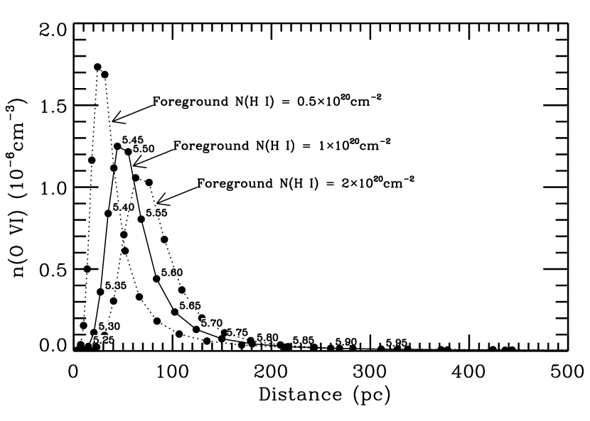
Figure 5: The density of O VI vs. distance along our line of sight for the hypothetical case where all of the regions are arranged in an end-to-end sequence from low to high temperature. The solid curve represents our solution to the power-law temperature (or length-scale) relation for a foreground absorption equivalent to $N_{\rm HI}=1.0\times 10^{20}{\rm cm}^{-2}$, $p_{th}/k=8320\,{\rm cm}^{-3}$K, and $\beta=1.48$. On this curve, points are labeled according to their respective values of $\log T$. The other (dotted) curves represent other values of foreground absorption, as indicated (with $p_{th}/k$ and $\beta$ in each case set to the respective optimum values - see Table 4).

On the one hand, it is important to note that $L$ represents a minimum length scale, since parcels of gas could be scattered over a longer distance with some unseen gas phase filling in the intervening gaps. On the other hand, the fraction of $L$ that has an appreciable concentration of O VI is small. Figure 5 illustrates what the concentration of O VI would look like if all of the gas parcels at different temperatures were sequenced along a line in order of increasing temperature. Most of the O VI-bearing gas is confined within a region that is less than about 100 pc thick, with the remaining, much greater length filled with a plasma that is too hot to contain much O VI. This thickness is considerably less than the 2.3 kpc scale height found for O VI in the Galactic halo by Savage et al. (2003). Evidently, our large observed ratio of $I_{\rm OVI}/N_{\rm OVI}$ shows that the gas with temperatures of around 300,000 K is highly clumped, even when one acknowledges that there can be a broad distribution of temperatures. The internal densities $n({\rm OVI})$ within each clump, which in our model can reach as high as $\sim 10^{-6}~{}{\rm cm}^{-3}$, is about two orders of magnitude higher than an overall average $<n({\rm OVI})>=1.7\times 10^{-8}{\rm cm}^{-3}$ that was found in a FUSE  survey of the Galactic disk (Bowen et al., 2006).

The column density of electrons along our line of sight is given by

$$N_{e}=B\int_{\ln 10^{5}\rm{K}}^{\ln T_{\rm cut}}n_{e}(T)T^{\beta}d\ln T={p\over 1.92k}~{}{B(T_{\rm cut}^{\beta-1}-T^{5(\beta-1)})\over\beta-1}~{},$$ (14)

and we list outcomes for the appropriate values of $\beta$ and $N_{\rm HI}$ in Table 4.

In §3.1 we discussed the possibility that the abundance of oxygen might be higher than the one that we adopted from Asplund et al. (2004). If we were to adopt the old, higher abundance value given by Grevesse & Sauval (1998) (larger by 0.27 dex), the values of $\beta$ listed in Table 4 would increase by about 0.5 because the relative proportion of the plasma at temperatures that emit O VI line radiation is reduced, when compared to the higher temperature material that emits soft X-rays. (Recall that the predicted X-ray emission is not strongly influenced by changes in the abundance of oxygen, as we stated in an earlier footnote.) For the three values of foreground $N$(H I), (0.5, 1.0, $2.0\times 10^{20}\,{\rm cm}^{-2}$), the old oxygen abundance changes $\log p_{th}/k$ by (+0.03, +0.03, +0.05) dex, respectively. Values of $\log L$ change by (+0.23, +0.09, +0.17) dex, while $\log N_{e}$ changes by (+0.05, +0.01, +0.03) dex.

3.5.4 The Total Radiative Loss Rate for the Halo

Here, we assume that the observed line of sight provides a fair representation of the halo as a whole. This assumption allows us to calculate the total radiative energy loss rate associated with hot gas in the halo, a rate that can be usefully compared with the energy injection rate.

To compute the radiative energy loss rate from the hot gas in the halo, we must know how the differential emission measure $dEM=n_{e}^{2}(T)dl$ varies with temperature. With our reformulation of $dl$ in terms of $d\ln T$ we find that

$$dEM(T)=\left({p_{th}\over 1.92k}\right)^{2}BT^{\beta-2}d\ln T$$ (15)

along our line of sight. The second to the last group of numbers in Table 4 shows the logarithms of the coefficient in front of the $T^{\beta-2}$ term in the equation.

With our expression for the emission measure as a function of $T$, we are now prepared to estimate the power radiated by the gas at temperatures above $10^{5}\,$K. For a cooling function $\Lambda_{N}$ that is normalized to the local product of electron and ion densities $n_{e}n_{i}$, we adopt the values listed by Sutherland & Dopita (1993) that apply to a plasma that has a solar composition and nonequilibrium ion fractions in a regime of radiative, isochoric cooling, starting with an initial temperature of $10^{7.5}\,$K. If we were to suppose that our line of sight shows a fair representation of the cooling per unit area $dU/dt$ by hot gas on both sides of the Galactic plane in our region of the Galaxy, we find that

$$dU/dt=2\sin(|b|)(0.917)\int_{\ln 10^{5}\rm{K}}^{\ln T_{\rm cut}}EM(T)\Lambda_{N}d\ln T$$ (16)

where $b$ is the Galactic latitude of our line of sight ($-47\fdg 1$), the factor 2 accounts for both sides of the plane, and the factor 0.917 allows for the fact that our expression for $EM(T)$ is cast in terms of $n_{e}^{2}$ whereas the normalization of the function expressed by Sutherland & Dopita (1993) is normalized to $n_{e}n_{i}$. Values of $\log dU/dT$ are listed in the last group of numbers in Table 4. Several important qualifications must be expressed about these numbers. First, we have truncated the calculation at a lower limit $T=10^{5}\,$K because we have no ability to sense gas at lower temperatures. If an extrapolation of our power-law representation seems plausible, we should expect to find some additional energy radiated below $10^{5}\,$K. This is demonstrated in Fig. 6, where we have plotted the shape of the integrand in Eq. 16 as a function of $\log T$. Second, Sutherland & Dopita (1993) used the solar abundances given by Anders & Grevesse (1989) instead of the more modern values of Allende Prieto, Lambert, & Asplund (2002) that we adopted. Thus, if the function $\Lambda_{N}$ were to be recalculated using the newer abundances, we would find a somewhat lower cooling rate, but by a factor that is less severe than the changes in the C, N and O abundances, since other elements are also important coolants. If indeed the older abundances are correct, the ripple effect from the changes in the parameters derived in §3.5 above could reduce the emission power by up to -0.4 dex. Aside from these possible offsets, our determination should be free of bias, and indeed the values of O VI and X-ray emission found here are fairly typical of those found along other high latitude sight lines. Nevertheless, it is important to note that the distribution of hot gas in the Galactic halo is extremely uneven; hence our single line of sight does not give a very accurate representation of the average $EM$ on either side of the Galactic plane.

The rate of cooling, $dU/dt$, is similar to the rate of energy input from supernova explosions and pre-supernova winds. The average massive SN progenitor star releases $1.4$ to $2.0\times 10^{50}$ ergs in wind energy before it explodes, according to calculations in Ferrière (1998) and Leitherer, Robert & Drissen (1992). At the Sun’s galactocentric radius, 18.6 massive stars and 2.6 white dwarfs explode per Myr per kpc² cross-sectional disk area, though many of these stars explode above the disk (Ferrière, 1998). If each explosion releases $10^{51}$ ergs of energy, then SN and pre-SN winds inject $7.66$ to $8.06\times 10^{38}$ erg kpc^-2 s^-1 into the ISM. A comparison with the calculated energy loss rate for our nominal case ($5.37^{+0.80}_{-0.69}\times 10^{38}$ erg kpc^-2 s^-1) shows that the majority of the injected SN and pre-SN energy is later radiated away by hot halo gas. Since the halo cooling rate accounts for $\sim 70\%$ of the SN and pre-SN wind energy injection rate, little remains to power other activities, such as large scale galactic winds. Half of the photons emitted by the halo will travel toward the galactic midplane and likely be absorbed, while the other half will travel upwards. Their absorption rate depends on the column density of gas residing above the emitting gas, which is expected to be less than $\sim 1\times 10^{20}$ cm^-20. Thus, most of the 1032 Å and shorter photons will leave the system.

4 Summary

We analyzed FUSE LWRS data for $\ell=278.7^{\rm{o}},b=-47.1^{\rm{o}}$, finding an O VI doublet intensity of 4710 $\pm$ 570 photons cm^-2 s^-1 sr^-1. Our pointing direction is only mildly extincted, so the observed intensity included contributions from the Local Bubble and the Galactic halo. Only $2^{\rm{o}}$ from our pointing direction, the sky is heavily extincted by a filament residing 230 pc from the Earth. A previous observation of that direction indicated the Local Bubble’s contribution. The difference between the intensities observed on these two sight lines, $4680^{+570}_{-660}$ photons cm^-2 s^-1 sr^-1, can be attributed to the halo. Given the extinction along our line of sight due to an $N_{\rm{HI}}$ of 0.5 to $2.0\times 10^{20}$ cm^-2, the halo’s intrinsic intensity is $5350^{+650}_{-750}$ to $7960^{+970}_{-1120}$ photons s^-1 cm^-2 sr^-1.

We estimated the halo’s O VI column density from absorption lines seen in the UV spectra of extragalactic objects. We averaged values toward the 4 nearest sight lines and then subtracted an estimate for the expected contribution from the Local Bubble. When we used it and our intrinsic O VI intensity range and treated the O VI-bearing gas as if it were isothermal, we found that the electron density and thermal pressure in the halo’s O VI-rich gas are 0.01 to 0.02 cm^-3 and 7000 to 10,000 K cm^-3, respectively.

By performing a similar shadowing analysis with the ROSAT 1/4 keV data, we determined the 1/4 keV count rate attributable to the Galactic halo along $\ell=278.7^{\rm{o}},b=-47.1^{\rm{o}}$. It is 732 $\pm$ 142 $\times 10^{-6}$ counts s^-1 arcmin^-2, before accounting for line of sight extinction. After accounting for extinction, the intrinsic R12 countrate is $779\pm 151$ to $4770\pm 930$ counts s^-1 arcmin^-2. The O VI vs 1/4 keV intensity ratio is 4.7 to 1.1, depending on whether the emitting gas is beyond $N_{\rm{HI}}=0.5$ or $2.0\times 10^{20}$ cm^-2, respectively. Thus, more energy leaves the system through the O VI resonance lines than through the ROSAT 1/4 keV bandpass. In contrast, the opposite is true of the local region (Local Bubble $+$ heliospheric), where roughly twice as much energy (at least) is radiated by the 1/4 keV emission lines than by the O VI resonance line doublet.

In order to estimate the maturity of the emitting plasma, we compared the O VI to soft X-ray ratio with predictions for a simulated supernova remnant at various times in its life. Around the time that the thermal temperature throughout most of the remnant approached the plasma’s collisional ionizational equilibrium temperature, the spectrum produced a 4.7 to 1 ratio, coincident with the observational ratio assuming minimal extinction. Earlier in its life, the simulated remnant had produced a 1.1 to 1 ratio, coincident with the observational ratio assuming mild extinction. Specifically, these ratios were achieved when the SNR was 70,000 and 40,000 years old, respectively. We suggest that other possible hot gas structures would be similarly mature when they, too, produce a similar O VI to soft X-ray intensity ratio.

Using the O VI to soft X-ray ratio, we were also able to parameterize the hot halo plasma with a power law temperature distribution ($dl=BT^{\beta}d\ln T~{}{\rm for}~{}10^{5}\,{\rm K}<T<T_{\rm cut}$). Given the nominal estimates of foreground absorption ($N_{\rm HI}=1.0\times 10^{20}$ cm^-2) and O VI column density ($N_{\rm OVI}=2.09\times 10^{14}$ cm^-2) along our line of sight, we found $\beta=1.48\pm 0.18$, $T_{\rm cut}=10^{6.6}$ K, and $B=10^{-6.16\pm 0.37}$ K^-β pc. Hot gas with a temperature between $10^{5}$ K and $T_{\rm cut}$ occupies $\int dl=10^{3.44\pm 0.37}$ pc along our line of sight, but the O VI-rich gas occupies a small fraction of this length. Assuming that our line of sight is typical of high latitude sight lines, we found the cooling rate for the halo (both sides of the plane beyond the Local Bubble) per unit cross sectional area to be $dU/dt=10^{38.73\pm 0.06}$ erg s^-1 kpc^-2. At the Sun’s galactocentric radius, the hot halo’s radiative cooling accounts for $\sim 70\%$ of the energy injected into the ISM from SNe and pre-SN winds in the galactic disk and halo. The remaining $\sim 30\%$ of the injected energy must be split between all other energy loss processes.

Table 1: Observed Intensities and 1 $\sigma$ Statistical Uncertainties

	Night Only	Night Only	Day+Night	Day+Night
	Method $\#$1	Method $\#$2	Method $\#$1	Method $\#$2
	(ph s-1 cm-2 sr-1)	(ph s-1 cm-2 sr-1)	(ph s-1 cm-2 sr-1)	(ph s-1 cm-2 sr-1)
O VI 1032 Å	3270 $\pm$ 460	3150 $\pm$ 540	3150 $\pm$ 350	3680 $\pm$ 420
O VI 1038 Å	1440 $\pm$ 380	2600 $\pm$ 630	1490 $\pm$ 280	1620 $\pm$ 380
C II∗ 1037 Å	1550 $\pm$ 330	1550 $\pm$ 400	1700 $\pm$ 250	1910 $\pm$ 300
1031 Å feature	–	–	1770 $\pm$ 260	1770 $\pm$ 270

Table 2: Velocity with Respect to the Local Standard of Rest

	Night Only	Night Only	Day+Night	Day+Night
	Method $\#$1	Method $\#$2	Method $\#$1	Method $\#$2
	(km sec-1)	(km sec-1)	(km sec-1)	(km sec-1)
O VI 1032 Å	28	25 $\pm$ 10	22	14 $\pm$ 10
O VI 1038 Å	-20	-24 $\pm$ 30	-5	-2 $\pm$ 10
C II∗ 1037 Å	-24	-31 $\pm$ 10	-17	-13 $\pm$ 10

Table 3: Physical Parameters of Halo O VI-rich Gas, Isothermal Case

Assumed $N_{\rm H}$	Transmission	$I_{\rm OVI}$	$N_{\rm OVI}$	$n_{e}$	$p_{th}/k$
				$\Delta l$	$t_{cool}$
($10^{20}$ cm-2)		(ph s-1 cm-2 sr-1)	(ions cm-2)	(cm-3)	(K cm-3)
				(pc)	(years)
$0.5$	88$\%$	$5350^{+650}_{-750}$	$2.09\pm 0.84\times 10^{14}$	$0.0110^{+0.0046}_{-0.0047}$	$6740^{+2820}_{-2860}$
				$69.8^{+56.8}_{-56.5}$	$7.36^{+3.13}_{-3.08}\times 10^{6}$
$1.0$	$77\%$	$6110^{+740}_{-860}$	”	$0.0125^{+0.0052}_{-0.0053}$	$7690^{+3220}_{-3270}$
				$61.1^{+49.7}_{-49.5}$	$6.45^{+2.74}_{-2.70}\times 10^{6}$
$2.0$	59$\%$	$7960^{+970}_{-1120}$	”	$0.0163^{+0.0068}_{-0.0069}$	$10040^{+4200}_{-4260}$
				$46.8^{+38.1}_{-37.9}$	$4.94^{+2.10}_{-2.07}\times 10^{6}$

Note. — Table is “line-wrapped”; $\Delta l$ and $t_{cool}$ appear below $n_{e}$ and $p_{th}/k$.

Table 4: Parameters for the Temperature Power Law

		Foreground $N({\rm H~{}I})~{}(10^{20}{\rm cm}^{-2})$
Parameter		0.5	1.0	2.0	Eq. nr.
$\beta$		$1.15\pm 0.20$	$1.48\pm 0.18$	$1.95\pm 0.17$	9
$\log T_{\rm cut}~{}({\rm K})$		6.9	6.6	6.4	10
$\log p_{th}/k~{}({\rm cm}^{-3}\,$K)	($\beta+$)	$3.86\pm 0.19$	$3.93\pm 0.19$	$4.08\pm 0.19$	11
	($\beta$)	$3.85\pm 0.19$	$3.92\pm 0.19$	$4.06\pm 0.19$
	($\beta-$)	$3.84\pm 0.19$	$3.91\pm 0.19$	$4.05\pm 0.19$
$<v^{2}>~{}({\rm km}^{2}{s}^{-2})$	($\beta+$)	208	225	259	12
	($\beta$)	198	214	242
	($\beta-$)	191	205	229
$\log B~{}({\rm K}^{-\beta}{\rm pc})$	($\beta+$)	$-5.37\pm 0.37$	$-7.12\pm 0.37$	$-9.95\pm 0.37$	4
	($\beta$)	$-4.25\pm 0.37$	$-6.16\pm 0.37$	$-8.92\pm 0.37$
	($\beta-$)	$-3.14\pm 0.37$	$-5.15\pm 0.37$	$-7.96\pm 0.37$
$\log L$ (pc)	($\beta+$)	$3.81\pm 0.37$	$3.56\pm 0.37$	$3.36\pm 0.37$	13
	($\beta$)	$3.62\pm 0.37$	$3.44\pm 0.37$	$3.26\pm 0.37$
	($\beta-$)	$3.43\pm 0.37$	$3.31\pm 0.37$	$3.18\pm 0.37$
$\log N_{e}~{}({\rm cm}^{-2})$	($\beta+$)	$19.46\pm 0.19$	$19.46\pm 0.19$	$19.50\pm 0.19$	14
	($\beta$)	$19.34\pm 0.19$	$19.37\pm 0.19$	$19.43\pm 0.19$
	($\beta-$)	$19.25\pm 0.19$	$19.30\pm 0.19$	$19.36\pm 0.19$
$\log[dEM(T)T^{2-\beta}/d\ln T]$	($\beta+$)	$1.78\pm 0.06$	$0.18\pm 0.06$	$-2.36\pm 0.06$	15
$({\rm K}^{\beta-2}{\rm cm}^{-6}{\rm pc})$	($\beta$)	$2.88\pm 0.06$	$1.12\pm 0.06$	$-1.36\pm 0.06$
	($\beta-$)	$3.98\pm 0.06$	$2.11\pm 0.06$	$-0.42\pm 0.06$
$\log(dU/dt)~{}({\rm erg~{}s}^{-1}{\rm kpc}^{-2})$	($\beta+$)	$38.69\pm 0.06$	$38.76\pm 0.06$	$38.72\pm 0.06$	16
	($\beta$)	$38.73\pm 0.06$	$38.73\pm 0.06$	$38.78\pm 0.06$
	($\beta-$)	$38.77\pm 0.06$	$38.76\pm 0.06$	$38.79\pm 0.06$

Note. — Errors appended to the listed quantities are the formal errors that arise from uncertainties in the measured quantities only. They do not include systematic errors caused by inaccuracies in atomic physics parameters, element abundances, the assumption of isobaric conditions, or deviations from our temperature power-law representation.

Figure 2: LiF1A spectra, binned by 0.065 Å and plotted relative to the corrected wavelength for the Local Standard of Rest (LSR) reference frame. Top panel: spectrum from the satellite-night portion of the data. Bottom panel: spectrum from the full dataset. The O VI 1032 and 1038 Å emission lines and the C II^∗ emission line appear in both the night only and the day+night spectra. The feature at 1031.2 Å in the day+night spectrum may be the second order diffraction of an atmospheric emission feature of He I at 515.62 Å. It, like the Earth’s airglow emission lines (marked with crossed circles), appear much brighter in the day+night spectrum than in the night-only spectrum.

Figure 3: The range of observationally derived O VI to 1/4 keV intensity ratios (dot-dash line to dashed line) are compared with the predicted ratio from an evolving supernova remnant (thick solid line) and the remnant’s average ratio (dotted line). The SNR’s O VI to soft X-ray intensity ratio reaches 1.1 (dot-dash line) when the remnant is about 40,000 years old and reaches 4.7 (dashed line) when the remnant is about 70,000 years old. The observationally determined ratio (1.1 to 4.7) is less than the remnant’s lifetime averaged intensity weighted O VI to 1/4 keV ratio (8.9, dotted line). Also plotted on the graph is the time period when the remnant evolves from the adiabatic (Sedov) phase to the radiative phase. This phase is bracketed by vertical lines on the plot.

Figure 4: Plots that indicate the sensitivity of various physical parameters on the values of observed quantities. The three columns of panels represent solutions of the equations assuming different values for the foreground absorption, represented by $N_{\rm HI}$: (left) $0.5\times 10^{20}$ cm^-2, (middle) $1.0\times 10^{20}$ cm^-2, and (right) $2.0\times 10^{20}{\rm cm}^{-2}$cm^-2. In all of the plots, curves for different assumed values of $T_{\rm cut}$ are drawn in different styles: solid curves: $\log T_{\rm cut}=8.0$; dashed curves: $\log T_{\rm cut}=6.9$; dash-dot curves: $\log T_{\rm cut}=6.6$; dotted curves: $\log T_{\rm cut}=6.4$. Top row: The dependence of $\beta$ on the value of $I_{\rm OVI}/R_{12}$ in units of O VI photons arcmin² R12 counts^-1 sr^-1, as defined in Eq. 9. From the intersection of the observed value of this ratio (horizontal dotted line) and the curves, we obtain the best values of $\beta$ in each case (vertical dotted lines dropped down to the $\beta$ scales at the bottom). Second row: The dependence of $T_{\rm cut}$ on $R_{67}/R_{12}$ as a function of $\beta$, as defined by Eq. 10. We used these curves to define appropriate values of $T_{\rm cut}$ in each case by locating the one that most closely intersects the horizontal dotted line representing the observation at the preferred value of $\beta$. Third row: The expected ratio $(I_{\rm OVI}/N_{\rm OVI})/(p_{th}/1.92k)$ as a function of $\beta$, as expressed in Eq. 11. The intersections of the dotted lines show the outcomes for the best $\beta$ values with the thermal pressures listed in Table 4. Bottom row: The expected velocity variance as a function of $\beta$, as defined in Eq. 12.

Figure 6: Radiative energy loss rates per unit area, $dU/dt$, as a function $\log T$ for the preferred values of $\beta$ that apply to the three possible values of the foreground $N$(H I) (see Table 4). The curves plotted represent the product of the integrand and constants given in Eq. 16.

References

- Allende Prieto, Lambert, & Asplund (2002) Allende Prieto, C., Lambert, D. L., & Asplund, M. 2002, ApJ, 573, L137
- Anders & Grevesse (1989) Anders, E., & Grevesse, N. 1989, Geochim. Cosmochim. Acta, 53, 197
- Antia & Basu (2005) Antia, H. M., & Basu, S. 2005, ApJ, 620, L129
- Antia & Basu (2005) Antia, H. M., & Basu, S. 2006, ApJ, 644, 1292
- Asplund et al. (2005) Asplund, M., Grevesse, N., Güdel, M., & Sauval, A. J. 2005, astro-ph/0510377
- Asplund et al. (2004) Asplund, M., Grevesse, N., Sauval, A. J., Allende Prieto, C., & Kiselman, D. 2004, A&A, 417, 751
- Avillez & Breitschwerdt (2004) de Avillez, M. A., & Breitschwerdt, D. 2004, A & A, 425, 899
- Badnell et al. (2005) Badnell, N. R., Bautista, M. A., Butler, K., Delahaye, F., Mendoza, C., Palmeri, P., Zeippen, C. J., & Seaton, M. J. 2005, MNRAS, 360, 458
- Bahcall & Serenelli (2004) Bahcall, J. N., & Serenelli, A. M. 2004, ApJ, 621, L85
- Bahcall et al (2004) Bahcall, J. N., Basu, S., Pinsonneault, M., & Serenelli, A. M. 2004, ApJ, 618, 1049
- Bowen et al. (2006) Bowen, D. V., Jenkins, E. B., Tripp, T. M., Sembach, K. R., & Savage, B. D. 2006, ”Astrophysics in the Far Ultraviolet: Five Years of Discovery with FUSE”, Edited by G. Sonneborn, H. Moos, & B.-G. Andersson, p. 412
- Bloch et al. (1986) Bloch, J. J., Jahoda, K., Juda, M., McCammon, D., Sanders, W. T., Snowden, S. L 1986, ApJ, 308, 59
- Breitschwerdt & Cox (2004) Breitschwerdt, D., & Cox, D. P. 2004, “How Does the Galaxy Work? A Galactic Tertulia with Don Cox and Ron Reynolds”, Edited by Emilio J. Alfaro, Enrique Perez, & Jose Franco, p. 391
- Cox & Reynolds (1987) Cox, D. P., & Reynolds, R. J. 1987, ARAA, 25, 303
- Cunha et al (2006) Cunha, K., Hubeny, I., & Lanz, T. 2006, ApJ, 647, L143
- Daflon & Cunha (2004) Daflon, S., & Cunha, K. 2004, ApJ, 617, 1115
- Daflon et al (2003) Daflon, S., Cunha, K., Smith, V. V., & Butler, K. 2003, A&A, 399, 525
- Davidsen (1993) Davidsen, A. F. 1993, Science, 259, 327
- Diplas & Savage (1994) Diplas, A., & Savage, B. D. 1994, ApJ, 427, 274
- Dixon, Kruk & Murphy (2002) Dixon, W. V., Kruk, J. W., & Murphy, E. M. 2002, CALFUSE Pipeline Reference Guide, http:fuse.pha.jhu.eduanalysispipelinereference.html
- Dixon et al. (2001) Dixon, W. V., Sallmen, S., Hurwitz, M., & Lieu, R. 2001, ApJ, 552, L69
- Dixon et al. (2006) Dixon, W. V., Sankrit, R., & Otte, B., 2006, ApJ, 647, 328
- Drake & Testa (2005) Drake, J. J., & Testa, P. 2005, Nature, 436, 525
- Edvardsson et al (1993) Edvardsson, B., Anderson, J., Gustafsson, B., Lambert, D. L., Nissen, P. E., & Tomkin, J. 1993, A&A, 275, 101
- Esteban et al (2005) Esteban, C., García-Rojas, J., Peimbert, M., Peimbert, A., Ruiz, M. T., & Rodríguez, M. 2005, ApJ, 618, L95
- Ferrière (1998) Ferrière, K. 1998, ApJ, 503, 700
- Fitzpatrick (1999) Fitzpatrick, E. L. 1999, PASP, 111, 63
- Gaetz, Edgar, & Chevalier (1988) Gaetz, T. J., Edgar, R. J., & Chevalier, R. A. 1988, ApJ, 329, 927
- Grevesse & Anders (1989) Grevesse, N., & Anders, E. 1989, in AIP Conf. Proc. 183, Cosmic Abundances
- Grevesse & Sauval (1998) Grevesse, N., & Sauval, A. J. 1998, Space Sci. Rev., 85, 161
- Henley, Shelton & Kuntz (2006) Henley, D. B., Shelton, R. L., & Kuntz, K.D. 2006, in preparation
- Holweger (2001) Holweger, H. 2001, in Solar and Galactic Composition, A Joint SOHO/ACE Workshop (ed. Wimmer-Schweingruber, R. F.) (AIP, New York), p. 23
- Hurwitz & Bowyer (1993) Hurwitz, M., & Bowyer, S. 1996, ApJ, 465, 296
- Jenkins (1978) Jenkins, E. B. 1978, ApJ, 220, 107
- Kalberla et al (2005) Kalberla, P. M. W., Burton, W. B., Hartmann, D., Arnal, E. M., Bajaja, E., Morras, R., & Pöppel, W. G. L. 2005, A & A, 440, 775
- Kato (1976) Kato, T. 1976, ApJS, 30, 397
- Korpela et al. (2006) Korpela, E. J.,Edelstein, J., Kregenow, J., Nishikida, K., Min, K.-W., Lee, D.-H., Ryu, K., Han, W., Nam, U.-W., Park, J.-H. 2006, ApJ, 644, 163L
- Kuntz & Snowden (2000) Kuntz, K. D., & Snowden, S. L. 2000, ApJ, 543, 195
-
Lallement et al. (2003)
Lallement, R., Welsh, B. Y., Vergely, J. L., Crifo, F., & Sfeir, D.
2003, A & A, 411, 447
- Lallement (2004) Lallement, R., 2004, A & A, 418, 143
- Lecavelier des Etangs et al. (2004) Lecavelier des Etangs, A., Gopal-Krishna, & Durret, F., 2004, A & A, 421, 503L.
- Leitherer, Robert & Drissen (1992) Leitherer, C., Robert, C., & Drissen, L., 1992, ApJ, 401, 596
- Martín-Hernández et al (2002) Martín-Hernández, N. L., Peeters, E., Morisset, C., Tielens, A. G. G. M., Cox, P., Roelfsema, P. R., Baluteau, J.-P., Schaerer, D., Mathis, J. S., Damour, F., Churchwell, E., & Kessler, M. F. 2002, A&A, 381, 606
- Mazzotta et al. (1998) Mazzotta, P., Mazzitelli, G., Colafrancesco, S., & Vittorio, N. 1998, A & AS, 133, 403
- McCammon & Sanders (1990) McCammon, D., & Sanders, W. T. 1990, ARAA, 28, 657
- Miyaji et al. (1998) Miyaji, T., Ishisaki, Y., Ogasaka, Y., Ueda, Y.., Freyberg, M. J., Hasinger, G., & Tanaka, Y. 1998, A & A, 334, L13
- Morton (1991) Morton, D. C. 1991, ApJS, 777, 119
- Murthy et al. (2001) Murthy, J., Henry, R. C., Shelton, R. L., & Holberg, J.B. 2001, ApJ, 557, 47
- Nahar & Pradhan (2003) Nahar, S. N., & Pradhan, A. K. 2003, ApJS, 149, 239
- Otte & Dixon (2006) Otte, B., & Dixon, W. V., 2006, ApJ, 647, 312
- Peimbert (1999) Peimbert, M. 1999, in Chemical Evolution from Zero to High Redshift, ed. J. R. Walsh & M. R. Rosa (Berlin: Springer), p. 30
- Penprase et al. (1998) Penprase, B. E., Lauer, J., Aufrecht, J., & Welsh, B. Y. 1998, ApJ, 492, 617
- Pietz et al. (1998) Pietz, J., Kerp, J., Kalberla, P., Burton, W. B., Hartmann, D., & Mebold, U. 1998, A & A, 332, 55
- Raymond & Smith (1977) Raymond, J. C., & Smith, B. W. 1977, ApJS, 35, 419
- Rolleston, Dufton & Fitzsimmons (1993) Rolleston, W. R. J., Dufton, P. L., & Fitzsimmons, A. 1993, A&A, 284, 72
- Sahnow et al. (2000) Sahnow, D. J., et al. 2000, ApJ, 538, L7
- Savage & Lehner (2006) Savage, B. D., & Lehner, N. 2006, ApJS, 162, 134
- Savage et al. (2003) Savage, B. D., et al. 2003, ApJS, 146, 125
- Schlegel, Finkbeiner, & Davis (1998) Schlegel, D. J., Finkbeiner, D. P., & Davis, M. 1998, ApJ, 500, 525
- Shelton et al (2001) Shelton, R. L. et al. 2001, ApJ, 560, 730
- Shelton (1999) Shelton, R. L. 1999, ApJ, 521, 217
- Shelton (2003) Shelton, R. L. 2003, ApJ, 589, 261
- Shull & Slavin (1994) Shull, J. M., & Slavin, J. D. 1994, ApJ, 427, 784
- Slavin (1989) Slavin, J. D. 1989, ApJ, 346, 718
- Snowden et al. (1991) Snowden, S. L., Mebold, U., Hirth, W., Herbstmeier, U., & Schmitt, J. H. M. 1991, Science, 252, 1529
- Snowden et al. (1997) Snowden, S. L., Egger, R., Freyberg, M. J., McCammon, D., Plucinsky, P. P., Sanders, W. T., Schmitt, J. H. M. M., Truemper, J., & Voges, W. 1997, ApJ, 485, 125
- Sutherland & Dopita (1993) Sutherland, R. S., & Dopita, M. A. 1993, ApJS, 88, 253
- Wakker et al (2003) Wakker, B. P., et al., 2003, ApJS, 146, 1
- Yao & Wang (2005) Yao, Y., & Wang, Q. D. 2005, ApJ, 624, 751