F-mode sensitivity kernels for flows

Abstract

We compute f-mode travel-time sensitivity kernels for flows. Using a two-dimensional model, the scattered wavefield is calculated in the first Born approximation. We test the correctness of the kernels by comparing an exact solution (constant flow), a solution linearized in the flow, and the total integral of the kernel. In practice, the linear approximation is acceptable for flows as large as about $400$ m/s.

I Introduction

The solar f modes are useful tools for studying perturbations that reside within the top $2$ Mm below the surface of the Sun, and have been used as diagnostics as such before (Duvall & Gizon, 2000). The linear forward problem of time-distance helioseismology is to calculate functions, or kernels, which give the sensitivity of travel-time measurements to small-amplitude perturbations in the Sun. For a discussion of this general procedure, which is the one that we will follow here, see Gizon & Birch (2002).

In this study we are interested in flow kernels, i.e. functions which give the sensitivity of travel-time measurements to steady, small amplitude, two-dimensional, spatially-varying horizontal flows. By flow kernel, we mean the function $K$ defined by

$$\tau_{\rm diff}({\mbox{\boldmath$x_{1}$}}|{\mbox{\boldmath$x_{2}$}})=\int\!\!\!\!\int\mbox{\boldmath$u$}({\mbox{\boldmath$x$}})\cdot\mbox{\boldmath$K$}(\mbox{\boldmath$\Delta$},{\mbox{\boldmath$x$}})\,{{\rm d}}^{2}{\mbox{\boldmath$x$}},$$ (1)

where $\tau_{\rm diff}$ is the difference in travel time for waves propagating in opposite directions between two fixed locations $x_{1}$ and $x_{2}$ on the surface, $\mbox{\boldmath$u$}=(u_{x},u_{y})$ is the two-dimensional flow vector, and the integral is over the position vector ${\mbox{\boldmath$x$}}=(x,y)$ that spans the whole solar surface. We adopt a cartesian geometry for the sake of simplicity. The kernel $\mbox{\boldmath$K$}=(K_{x},K_{y})$ is a two-dimensional vector which gives the sensitivity to flows in the $\hat{{\mbox{\boldmath$x$}}}$ and $\hat{\mbox{\boldmath$y$}}$ directions. Furthermore, we define $\mbox{\boldmath$\Delta$}={\mbox{\boldmath$x_{2}$}}-{\mbox{\boldmath$x_{1}$}}$ and the distance $\Delta=\|\mbox{\boldmath$\Delta$}\|$ between the two points $x_{1}$ and $x_{2}$.

In Section II we describe our simplified model of f-mode propagation through an inhomogeneous moving medium. In Section III, we consider a uniform flow and compare the exact solution, its linearization in the flow, and the third-order approximation. In Section IV, we show example kernels. We discuss the results in the last section.

II Zero-order wavefield and first Born approximation

In general, observations of solar oscillations are described by the filtered line-of-sight projection of the observed Doppler velocity $v$ given by

$$\psi({\mbox{\boldmath$x$}},t)={\cal F}[\mbox{\boldmath${\ell}$}\cdot\mbox{\boldmath$v$}]\equiv{\cal F}[\phi],$$ (2)

where the operator ${\cal F}$ describes the convolution with the point-spread function of the telescope and any additional filtering used in the data analysis, ${\ell}$ denotes the line-of-sight unit vector, and $\phi$ is the line-of-sight Dopplergram.

As was done by Gizon & Birch (2002), we consider a constant density half-space with a free surface at $z=0$. Gravitational acceleration, $-g\mbox{\boldmath$\hat{z}$}$, is constant. The medium is permeated by a steady, horizontal, divergenceless, and irrotational flow, $\mbox{\boldmath$u$}({\mbox{\boldmath$x$}})$. The condition $\mbox{\boldmath$\nabla$}\cdot\mbox{\boldmath$u$}=0$ is imposed by the continuity equation in the steady state. In addition, we require that $\mbox{\boldmath$\nabla$}\times\mbox{\boldmath$u$}=0$ to keep the problem two-dimensional. Under these conditions of smoothness, the fluid velocity remains irrotational at all times.

As is appropriate for solar waves, we consider small-amplitude (linear) waves. At the free surface $z=0$, the linearized dynamical and kinematic boundary conditions are

$$p/\overline{\rho}-g\eta = \Pi/\overline{\rho}\qquad z=0,$$ (3)

$$-{{\rm i}}\omega\eta+\mbox{\boldmath$u$}\cdot\mbox{\boldmath$\nabla$}\eta = \partial_{z}\Theta\qquad z=0,$$ (4)

where $\Theta$ is the wave velocity potential $\mbox{\boldmath$v$}=\mbox{\boldmath$\nabla$}\Theta$, $\eta$ is the elevation of the fluid’s surface, $p$ is a pressure perturbation, $\overline{\rho}$ is the background density, and $\Pi$ is a stochastic pressure source that generates the waves. The above equations and the following ones apply to quantities that were Fourier-transformed in time ($\omega$ is the angular frequency). In the bulk, the linearized momentum and continuity equations are

$$-{{\rm i}}\omega\Theta+\mbox{\boldmath$u$}\cdot\mbox{\boldmath$\nabla$}\Theta = -p/\overline{\rho}-\Gamma[\Theta],$$ (5)

$$\mbox{\boldmath$\nabla$}^{2}\Theta = 0,$$ (6)

where $\Gamma$ is a phenomenological frequency-dependent damping operator (Gizon & Birch, 2002).

In order to obtain the scattered wavefield computed in the first Born approximation, we expand any wave quantity $q$ into a zero-order term $q^{0}$ (in the absence of the flow) and a first-order term $\delta q$ caused by the flow perturbation. In the bulk, the velocity potentials $\Theta^{0}$ and $\delta\Theta$ both satisfy the three dimensional Laplace’s equation. Eliminating pressure and surface elevation, the zero-order and first-order surface boundary conditions at $z=0$ reduce to

$$(\partial_{z}-\kappa)\Theta^{0} =\frac{{{\rm i}}\omega}{\overline{\rho}g}\Pi\equiv S^{0},$$ (7)

$$(\partial_{z}-\kappa)\delta\Theta ={{\rm i}}\mbox{\boldmath$u$}\cdot\mbox{\boldmath$\nabla$}\left[(\partial_{\omega}\kappa)\Theta^{0}+\partial_{\omega}S^{0}\right]\equiv\delta S,$$ (8)

where $\kappa(\omega)=\omega^{2}/g+{{\rm i}}\gamma\omega/g$ is the complex wavenumber at resonance and $\gamma(\omega)$ is a realistic damping rate (Gizon & Birch, 2002). In doing so, we have used the approximations $\delta\Pi={{\rm i}}\mbox{\boldmath$u$}\cdot\mbox{\boldmath$\nabla$}\partial_{\omega}\Pi$ and $\delta\Gamma\Theta^{0}={{\rm i}}(\partial_{\omega}\gamma)\mbox{\boldmath$u$}\cdot\mbox{\boldmath$\nabla$}\Theta^{0}$, which describe the perturbations to the source of excitation and the wave damping respectively (this can be understood by transforming to a co-moving frame).

The solution of the zero- and first-order problems can be solved by introducing a Green’s function. The final result for the observable $\psi$ (on the surface) is

$$\psi^{0}({\mbox{\boldmath$x$}},\omega) ={\cal F}\left[(\ell_{\rm h}\cdot\mbox{\boldmath$\nabla$}_{\rm h}+\ell_{z}\kappa)\Theta^{0}\right],$$ (9)

$$\delta\psi({\mbox{\boldmath$x$}},\omega) ={\cal F}\left[(\ell_{\rm h}\cdot\mbox{\boldmath$\nabla$}_{\rm h}+\ell_{z}\kappa)\delta\Theta+{{\rm i}}\ell_{z}(\partial_{\omega}\kappa)\mbox{\boldmath$u$}\cdot\mbox{\boldmath$\nabla$}\Theta^{0}\right],$$ (10)

where $\mbox{\boldmath${\ell}$}=(\ell_{\rm h},\ell_{z})$, $\mbox{\boldmath$\nabla$}_{\rm h}$ is the horizontal gradient, and the zero-order and first-order surface velocity potentials are given by

$$\Theta^{0}({\mbox{\boldmath$x$}},\omega) =2\pi\int\!\!\!\int G({\mbox{\boldmath$x$}}-{\mbox{\boldmath$x$}}^{\prime},\omega)S^{0}({\mbox{\boldmath$x$}}^{\prime},\omega){{\rm d}}^{2}{\mbox{\boldmath$x$}}^{\prime},$$ (11)

$$\delta\Theta({\mbox{\boldmath$x$}},\omega) =2\pi\int\!\!\!\int G({\mbox{\boldmath$x$}}-{\mbox{\boldmath$x$}}^{\prime},\omega)\delta S({\mbox{\boldmath$x$}}^{\prime},\omega){{\rm d}}^{2}{\mbox{\boldmath$x$}}^{\prime},$$ (12)

with

$$G({\mbox{\boldmath$x$}},\omega)=\frac{1}{(2\pi)^{3}}\int\!\!\!\int\frac{e^{{{\rm i}}{\mbox{\scriptsize\boldmath$k$}}\cdot{\mbox{\scriptsize\boldmath$x$}}}}{k-\kappa(\omega)}\,{{\rm d}}^{2}\mbox{\boldmath$k$},$$ (13)

where $k=\|\mbox{\boldmath$k$}\|$ is the horizontal wavenumber. With the above expressions for the observed wavefield, one can compute the temporal cross-covariance function.

III Uniform flow: exact, first-, and third-order solutions

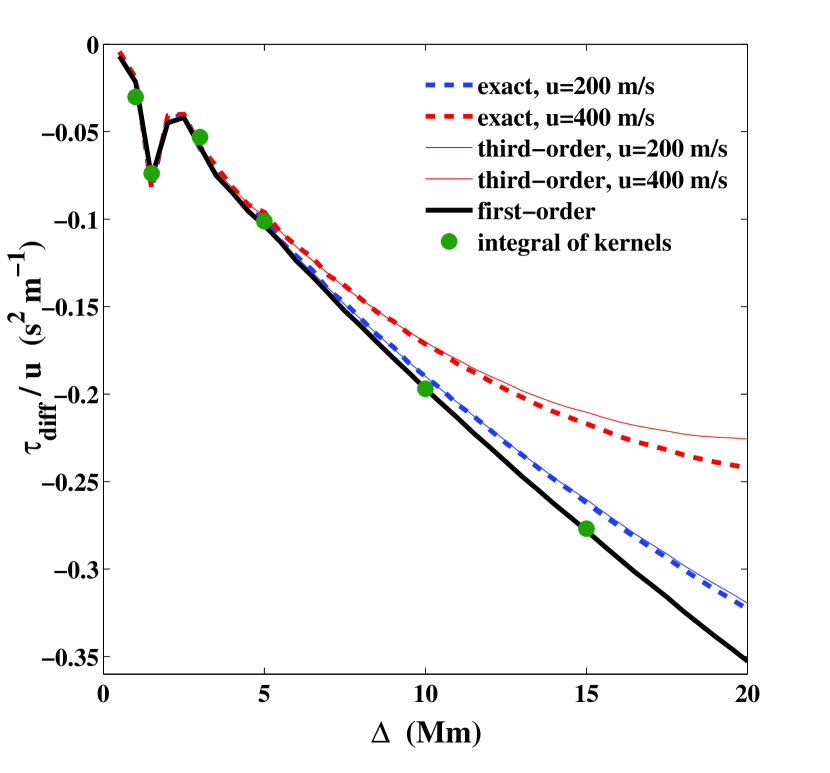
Figure 1: F-mode travel-time differences versus distance for uniform horizontal flows. Two values are chosen for the flow amplitude, $u=200$ m/s and $u=400$ m/s. The thick black solid line is the solution to the first-order approximation, the thin solid lines are the third-order solutions, and the dashed lines are the exact solutions. The green dots denote the values of the spatially-integrated kernels from Sec. IV.

Figure 2: F-mode travel-time differences versus uniform horizontal flow for different distances. Two distances are studied, $\Delta=5$ Mm and $\Delta=10$ Mm, given by the red and blue sets of curves respectively. For each set of curves, the thick solid line denotes the first-order solution, the thin solid line is the third-order solution, and the dashed line is the exact solution.

Before using the first-order Born approximation from the previous section to derive the sensitivity kernels (see Sec. IV), we wish to consider here the case of constant flows,

$$\mbox{\boldmath$u$}={\rm const}.$$ (14)

In this case, $\phi({\mbox{\boldmath$x$}},t)$ can be calculated simply by considering the Galilean transformation ${\mbox{\boldmath$x$}}\rightarrow{\mbox{\boldmath$x$}}-\mbox{\boldmath$u$}t$:

$$\phi({\mbox{\boldmath$x$}},t)=\phi^{0}({\mbox{\boldmath$x$}}-\mbox{\boldmath$u$}t,t).$$ (15)

This transformation applies to all other quantitites in the problem except for the filter ${\cal F}$. So the filtered wavefield in Fourier space is then given by

$$\psi(\mbox{\boldmath$k$},\omega)=F(\mbox{\boldmath$k$},\omega)\phi^{0}(\mbox{\boldmath$k$},\omega-\mbox{\boldmath$k$}\cdot\mbox{\boldmath$u$}),$$ (16)

where multiplication by $F(\mbox{\boldmath$k$},\omega)$ accounts for the action of the filter operator ${\cal F}$ in Fourier space. The filter contains a mode-mass correction which is the ratio of the mode inertia in our model to the mode inertia in a standard stratified model. In general it also contains a phase-speed filter, but in the particular case presented here where only f modes are excited, a phase-speed filter is unnecessary and therefore $F$ is independent of $\omega$.

The expectation value of the cross-covariance function is given by (Gizon & Birch, 2002)

$$C({\mbox{\boldmath$x_{1}$}}|{\mbox{\boldmath$x_{2}$}},\omega)=\int\!\!\!\int P(\mbox{\boldmath$k$},\omega)e^{{{\rm i}}{\mbox{\scriptsize\boldmath$k$}}\cdot{\mbox{\scriptsize\boldmath$\Delta$}}}\,{{\rm d}}^{2}\mbox{\boldmath$k$},$$ (17)

where

$$P(\mbox{\boldmath$k$},\omega)=E[|\psi(\mbox{\boldmath$k$},\omega)|^{2}]$$ (18)

denotes the expectation value of the power spectrum. In particular, the zero-order, or unperturbed ($\mbox{\boldmath$u$}=0$), cross-covariance is given by

$$C^{0}({\mbox{\boldmath$x_{1}$}}|{\mbox{\boldmath$x_{2}$}},\omega)=\int\!\!\!\int P^{0}(\mbox{\boldmath$k$},\omega)e^{{{\rm i}}{\mbox{\scriptsize\boldmath$k$}}\cdot{\mbox{\scriptsize\boldmath$\Delta$}}}\,{{\rm d}}^{2}\mbox{\boldmath$k$}.$$ (19)

Following Gizon & Birch (2002), the travel-time difference can be measured from the cross-covariance function according to

$$\tau_{\rm diff}({\mbox{\boldmath$x_{1}$}}|{\mbox{\boldmath$x_{2}$}})=\frac{-2{\rm Re}\int_{0}^{\infty}{{\rm i}}\omega C^{0}(\mbox{\boldmath$\Delta$},\omega)\,\Delta C(\mbox{\boldmath$\Delta$},\omega)\,{{\rm d}}\omega}{\int_{0}^{\infty}\omega^{\prime 2}|C^{0}(\mbox{\boldmath$\Delta$},\omega^{\prime})|^{2}\,{{\rm d}}\omega^{\prime}},$$ (20)

using $\Delta C=C-C^{0}$, where Re takes the real part of the expression. The travel-time shift $\tau_{\rm diff}({\mbox{\boldmath$x_{1}$}}|{\mbox{\boldmath$x_{2}$}})$, i.e., the difference in time it takes for waves going from $x_{1}$ to $x_{2}$ and for those going from $x_{2}$ to $x_{1}$. In our problem, $\tau_{{\rm diff}}$ is due to the flow.

On one hand, the travel-time difference may be computed exactly for any value of $u$. This is simply done numerically by using eqs. (16)-(20).

On the other hand, an approximation to the travel-time difference can be obtained by expanding the power spectrum as a Taylor series in $u$. This will provide us with a means to test the first-order Born approximation developed in Section II, as well as to quantify higher-order terms. For a constant flow, the Taylor expansion of the power spectrum (eq. [18]) is

$$P(\mbox{\boldmath$k$},\omega)= P^{0}(\mbox{\boldmath$k$},\omega)-\mbox{\boldmath$k$}\cdot\mbox{\boldmath$u$}|F|^{2}\partial_{\omega}|\phi^{0}|^{2}$$

$$+\frac{1}{2}(\mbox{\boldmath$k$}\cdot\mbox{\boldmath$u$})^{2}|F|^{2}\partial_{\omega}^{2}|\phi^{0}|^{2}$$

$$-\frac{1}{6}(\mbox{\boldmath$k$}\cdot\mbox{\boldmath$u$})^{3}|F|^{2}\partial_{\omega}^{3}|\phi^{0}|^{2}+\dots$$ (21)

We may truncate this expansion after each successive term to study the first-, second-, and third-order travel-time differences (using eq. [20]). The second-order term does not affect travel-time differences because it only introduces perturbations to the cross-covariance that are symmetric in the time lag.

Figure 2 shows the exact and approximate travel-time differences $\tau_{\rm diff}/u$ versus $\Delta$ computed at fixed $\mbox{\boldmath$u$}=u\hat{\mbox{\boldmath$\Delta$}}$ for $u=200$ m/s and $u=400$ m/s. We find that the first-order approximation is within 10% of the exact value for $\Delta<20$ Mm, while the error is only about 1% when terms up to $u^{3}$ are kept. For a flow that is twice as large, $u=400$ m/s, non-linear effects are more important. The non-linearity of $\tau_{\rm diff}$ with $u$ also increases as the separation distance $\Delta$ increases.

Figure 2 shows the variations of $\tau_{\rm diff}$ as a function of $u$ at fixed distances $\Delta=5$ Mm and $\Delta=10$ Mm. The first-order approximation is reasonable for flows with amplitudes less than about 400 m/s, although it gets worse for larger distances. In particular this means that the first-order approximation (and thus the kernels given in Sec. IV) is appropriate to study supergranular flows.

IV Sensitivity Kernels

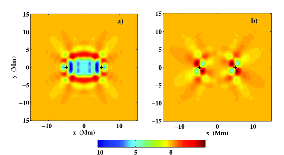
Figure 3: F-mode travel-time sensitivity kernels for flows. The separation distance of the observation points, denoted by the crosses, is $\Delta=10$ Mm. The coordinates are ${\mbox{\boldmath$x_{1}$}}=(-5,0)$ Mm and ${\mbox{\boldmath$x_{2}$}}=(5,0)$ Mm. The units of the colorscale are s Mm^-2/(km/s). The $K_{x}$ and $K_{y}$ components of the kernel are shown in panel a) and panel b) respectively.

We now return to the computation of sensitivity kernels in the first Born approximation in order to connect $\tau_{\rm diff}$ with a spatially varying flow $\mbox{\boldmath$u$}({\mbox{\boldmath$x$}})$.

The first-order perturbation to the travel time is obtained by approximating $\Delta C$ in eq. (20) by

$$\Delta C({\mbox{\boldmath$x_{1}$}},{\mbox{\boldmath$x_{2}$}},\omega)\simeq E\left[\delta\psi^{*}({\mbox{\boldmath$x_{1}$}},\omega)\psi^{0}({\mbox{\boldmath$x_{2}$}},\omega)\right.$$

$$+\left.\psi^{0*}({\mbox{\boldmath$x_{1}$}},\omega)\delta\psi({\mbox{\boldmath$x_{2}$}},\omega)\right].$$ (22)

The linear dependence of $\Delta C$ and $\tau_{\rm diff}$ on $u$ then follows from the expression of $\delta\psi$ (eq. [10]).

The kernel functions are identified according to their definition, eq. (1). The explicit expression of the flow kernels will be given in an upcoming publication.

A pair of sensitivity kernels is given in Fig. 3 for a distance $\Delta=10$ Mm (the observation points have coordinates ${\mbox{\boldmath$x_{1}$}}=(5,0)$ Mm and ${\mbox{\boldmath$x_{2}$}}=(-5,0)$ Mm). The kernel on the left, $K_{x}$, gives the sensitivity to $u_{x}$ and the kernel on the right, $K_{y}$, gives the sensitivity to $u_{y}$. The flow kernel $K_{x}$ displays elliptical and hyperbolic features, just as the kernels for the damping rate and the source strength derived earlier by Gizon & Birch (2002). The elliptical features have been called Fresnel zones in geophysics (e.g., (Tong et al., 1998)). The first Fresnel zone has a size (measured along $x=0$) which is roughly given by $(\lambda\Delta)^{1/2}$, where $\lambda\simeq 5$ Mm is the dominant f-mode wavelength. The hyperbolae are due to scattering of waves generated by distant excitation events. For reasons of symmetry (the $K_{y}$ kernel is antisymmetric with respect to the lines $x=0$ and $y=0$) the total integral of $K_{y}$ is zero.

For consistency, we have checked that the total integral of $K_{x}$ is nearly exactly the same (within 0.1%) as the first-order approximation of $\tau_{\rm diff}/u$ calculated under the assumption of a constant flow (Sec. III and Fig. 2). This gives us confidence in the numerics.

The effect of the line-of-sight projection of the Doppler velocity signal on the flow kernels are included in the model of Sec. II. This is not presented here, although it is briefly discussed in Jackiewicz et al. (2006).

V conclusions

Sensitivity kernels for flows have been calculated in the first Born approximation following the general recipe given by Gizon & Birch (2002).

It has proven very useful to consider a uniform flow model, which allows one to find an exact solution for the travel times, as well as approximations to the exact solution in leading powers of the flow $u$.

It was shown that the first-order solution is equivalent to the first Born approximation in the case of a uniform flow, and thus provides a test of the consistency of the kernels. This test revealed an accuracy within about 0.1%, giving us confidence in the numerical calculations. Furthermore, comparisons of the first-order solution with the exact solution show that it is reasonable to study flows up to 400 m/s, with the caveat that this value depends on the distance $\Delta$, with larger distances giving more error. Nonetheless, the linear model presented here is likely quite capable for the study of supergranular flows.

References

- Duvall & Gizon (2000) Duvall T. L., Gizon L., 2000, Sol. Phys. 192, 177
- Gizon & Birch (2002) Gizon L., Birch A. C., 2002, Astrophys. J. 571, 966
- Tong et al. (1998) Tong J., Dahlen F. A., Nolet G., Marquering H., 1998, Geophys. Res. Lett. 25, 1983
- Jackiewicz et al. (2006) Jackiewicz J., Gizon L., Birch A. C., 2006, in Ten Years of SOHO and Beyond, ESA SP-617, in press