Dark matter annihilation or unresolved astrophysical sources?
Anisotropy probe of the origin of cosmic gamma-ray background
Abstract
The origin of the cosmic gamma-ray background (CGB) is a longstanding mystery in high-energy astrophysics. Possible candidates include ordinary astrophysical objects such as unresolved blazars, as well as more exotic processes such as dark matter annihilation. While it would be difficult to distinguish them from the mean intensity data alone, one can use anisotropy data instead. We investigate the CGB anisotropy both from unresolved blazars and dark matter annihilation (including contributions from dark matter substructures), and find that the angular power spectra from these sources are very different. We then focus on detectability of dark matter annihilation signals using the anisotropy data, by treating the unresolved blazar component as a known background. We find that the dark matter signature should be detectable in the angular power spectrum of the CGB from two-year all-sky observations with the Gamma Ray Large Area Space Telescope (GLAST), as long as the dark matter annihilation contributes to a reasonable fraction, e.g., , of the CGB at around 10 GeV. We conclude that the anisotropy measurement of the CGB with GLAST should be a powerful tool for revealing the CGB origin, and potentially for the first detection of dark matter annihilation.
pacs:
95.35.+d; 95.85.Pw; 98.70.VcI Introduction
What is the energy budget of the GeV sky? The origin of the cosmic gamma-ray background (CGB) in the GeV region, which was discovered by the Energetic Gamma Ray Experiment Telescope (EGRET) Sreekumar1998 ; Strong2004a , is a longstanding mystery. Unresolved blazars, a beamed population of active galactic nuclei (AGNs), have been the most popular explanation for the CGB Padovani et al. (1993); Stecker1993 ; Salamon1994 ; Chiang et al. (1995); Stecker1996 ; Chiang & Mukherjee (1998); Mücke & Pohl (2000); Narumoto2006 ; Giommi2006 ; Dermer2006 ; however, even with the latest determination of the gamma-ray luminosity function (GLF), it has been shown that only 25–50% of the CGB can be explained by unresolved blazars alone Narumoto2006 . Other astrophysical sources include clusters of galaxies, from which gamma rays are emitted by either hadronic collisions between shock-accelerated protons and the surrounding medium Berezinsky1997 ; Colafrancesco1998 ; Pfrommer2003 or the inverse-Compton scattering of relativistic electrons off the cosmic microwave background (CMB) photons Loeb2000 ; Totani2000 ; Waxman2000 ; Keshet2003 ; Miniati2003 ; Gabici2003a ; Gabici2003b ; Gabici2004 . (Note, however, that such gamma rays have not been detected towards known clusters of galaxies yet Reimer2003 though there is some evidence Kawasaki2002 ; Scharf2002 .) The CGB may be solely coming from these two unresolved astrophysical sources at the comparable level for each, or other sources may be required to explain it.
What could be the other sources of the CGB? It is energetically easy to produce gamma-ray photons in the right energy region by decay or annihilation of heavy (i.e., 10 GeV or heavier) particles, the particles that have not been discovered yet. This possibility has been regarded as attractive because (i) more than 80% of matter in the universe is made of nonbaryonic dark matter, (ii) theories of supersymmetry predict that the lightest supersymmetric particles (e.g., neutralinos) are stable and are attractive candidates for dark matter (in the mass range of GeV to TeV), and (iii) these candidate dark matter particles can annihilate into GeV gamma rays Jungman1996 ; Bergstrom2000 ; Bertone2005a . The CGB flux from dark matter annihilation in cosmological dark matter halos has been calculated in the GeV Bergstrom2001 ; Ullio2002 ; Taylor2003 as well as in the MeV energies AK05a ; AK05b . Successive works have shown that this mechanism can account for a large fraction of the CGB with a reasonable choice of dark matter parameters, with a significant boost of the signal from substructures Oda2005 or minispikes around intermediate-mass black holes Horiuchi2006 (for the latter, see also Refs. Bertone2005b ; Bertone2006 ). In addition, with these boosts, we can also avoid an upper limit from the gamma-ray flux towards the Galactic Center Ando2005 . The excess of the CGB seen at around 3 GeV might be a signature of dark matter annihilation Elsaesser2005 .
Ando and Komatsu have recently shown that the angular power spectrum of anisotropy in the CGB may provide a smoking gun discovery of the annihilating dark matter Ando2006a (hereafter AK06). In that study the authors focused on the annihilation signal from dark matter halos with smooth density profiles. Only semi-quantitative arguments were given for the other astrophysical sources and the effects of dark matter substructures. We therefore investigate these two effects in detail in this paper, as they cannot be ignored if one wants to discuss whether anisotropy can really help detect the first signature of dark matter annihilation.
This paper is organized as follows. In Sec. II, we explain what the CGB intensity averaged over all the directions looks like, for both the dark matter annihilation (Sec. II.1) and blazars (Sec. II.2). We then turn our attention to the CGB anisotropy from dark matter substructure and blazars in Secs. III and IV, respectively, where we present formulation and results of the angular power spectrum. Section V is the main part of this paper, devoted to discussion concerning anticipated anisotropy analysis in the presence of components from both dark matter annihilation and blazars. We study the case of other astrophysical sources and discuss the robustness of our results in Sec. VI, and also give conclusions in the same section.
II Cosmic gamma-ray background: Mean intensity
In this section we calculate the mean intensity (i.e., intensity averaged over the directions) of the CGB from both dark matter annihilation (with substructures taken into account) and blazars, and compare the characteristics of these two components.
II.1 Dark matter annihilation
We include the effect of dark matter substructures as follows: we assume that substructures consist of a number of subhalos within a bigger host halo. These subhalos follow a certain mass function which is still unknown, but for our purpose we are only interested in quantities that are averaged over the mass function. If this mass function is independent of the halo position as we assume, these averaged subhalos having the same gamma-ray luminosity would follow a smooth density profile of a host halo such as the one proposed by Navarro, Frenk, and White (NFW) Navarro1996 ; Navarro1997 with a halo concentration parameter given in Ref. Bullock2001 . The gamma-ray profile of a halo thus traces the dark matter density, rather than the density squared which would be expected if dark matter distribution were smooth Ando2006a .
We define the number intensity, , as the number of photons emitted per unit area, time, solid angle, and energy range. In a general cosmological context, it is given by
| (1) |
where is the volume emissivity (energy of photons per unit volume, time, and energy range), is the Hubble function in a flat universe, and we assume the standard values for cosmological parameters, with , , and . We specify a certain direction by a unit vector, , position by a comoving distance vector, , and time by a redshift, (comoving distance, , is also used interchangeably). The exponential factor reflects the effect of gamma-ray absorption due to pair production with the extragalactic background light; such an effect is negligible in the energy range of interest here.
To evaluate the mean intensity, , we need . Let us define the gamma-ray spectrum per subhalo averaged over its mass function by , and the number of these subhalos within a parent halo of mass by . Then, we obtain the mean volume emissivity as
| (2) |
where is the mean comoving number density of subhalos given by
| (3) |
and is the halo mass function for which we use the expression given in Ref. Sheth1999 . The function, , includes all the particle physics parameters such as the annihilation cross section, , the dark matter mass , and the gamma-ray spectrum per annihilation . For the latter, we use a simple parameterization, i.e., , which is a good approximation for supersymmetric neutralino dark matter particles Bergstrom2001 . We parameterize the number of subhalos in each parent halo, which is also known as the Halo Occupation Distribution, as
| (4) |
If we ignore tidal destruction of subhalos entirely, we obtain , i.e., the number of subhalos is simply proportional to the mass of the parent halo. The tidal destruction should also change the gamma-ray emission profiles in the parent halo, as it works more strongly at inner halo regions. However, we adopt the NFW profile for all of our calculations, because the profile change should exert only secondary effect to our conclusions as discussed in Sec. III.2.
Using Eqs. (1) and (2), we obtain the mean intensity as follows:
| (5) |
where
| (6) |
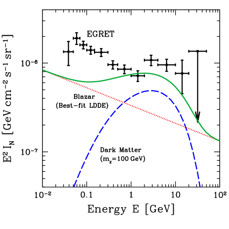
Figure 1 shows the CGB spectrum from dark matter annihilation, where the particle mass is assumed to be GeV. We do not give a specific value of or . These parameters are degenerate, but they do not affect predictions of the angular power spectrum, as we see below. All we require here is that the predicted intensity becomes comparable to the observed CGB, and this can be done by adjusting these two parameters. Previous work which included dark matter substructures Oda2005 has shown that this is indeed possible with a standard value of the annihilation cross section, cm3 s-1, which gives the right amount of the dark matter density in the universe if dark matter was thermally produced in the early universe Jungman1996 ; Bertone2005a . On the other hand, anisotropy depends only on and . We shall therefore vary and see how the results depend on , while we fix the mass at 100 GeV throughout the paper.
II.2 Blazars
If a non-negligible fraction of the CGB flux comes from astrophysical sources such as blazars and clusters of galaxies, they inevitably give a background (noise) for the dark matter detection in the anisotropy signature. It is thus very important to evaluate the contribution from the unresolved point sources. We concentrate on blazars as an example.
To calculate the mean CGB intensity from blazars one needs the GLF of blazars. We use the latest luminosity dependent density evolution (LDDE) model, which reproduces the observed GLF of the EGRET blazars better than a traditionally used pure luminosity evolution model Narumoto2006 . As the LDDE GLF was originally given for the luminosity at 100 MeV, we need to generalize it to the other energies. We do this by specifying the spectral shape; here we assume it to be a power law with a spectral index of Sreekumar1998 . Then, the luminosity per unit energy range, , is connected to the luminosity, ( at 100 MeV) adopted in the previous GLF via the following simple relation:
| (7) |
The GLF is accordingly replaced with the one defined as the comoving number density per unit range in , , which is related to the original one through
| (8) |
where we show the energy dependence of the new GLF explicitly by attaching subscript . Note that on the right hand side is given by Eqs. (8) and (10) of Ref. Ando2006b . Using Eqs. (7) and (8), we can rewrite the luminosity and the GLF at any energies as long as the spectrum is kept to be a power law with the same index.
The photon flux from the source with luminosity at redshift at energy is given by
| (9) |
where is the luminosity distance out to a source at . The flux sensitivity for point sources of the EGRET is cm-2 s-1 above 100 MeV Thompson1993 , and all the unresolved sources that give a flux below this threshold contribute to the CGB. The conversion from the differential flux per energy, , to the integrated flux, , can easily be performed by integrating over energy above 100 MeV and assuming the spectrum to be a power law with an index . One obtains
| (10) |
We use this equation and Eq. (9) to calculate the limiting source luminosity, , from .
We calculate the mean CGB intensity coming from unresolved blazars whose gamma-ray flux is below from
| (11) | |||||
where we use , and is the comoving volume per unit redshift and unit solid angle ranges. We show in Fig. 1 the CGB spectrum calculated with the best-fitting LDDE GLF together with the EGRET data. The predictions fall below the EGRET data, accounting for only 25–50% of the observed CGB Narumoto2006 ; Ando2006b .
This is presumably either because there is another class of objects which can contribute to the CGB by equally significant amount, or because the best-fitting LDDE model is underestimating the true GLF.111This may instead be because of underestimated contamination of the Galactic foreground emission Keshet2004a . For the former case, the particle acceleration in other astrophysical objects may also give a power-law CGB spectrum similar to that of blazars, and depending on its luminosity function, an unaccounted fraction of the CGB flux might be attributed to this population. Since the EGRET data may be explained by a power law component, such additional sources, plus blazars, might give almost full account of the CGB in the GeV region. One such candidate is galaxy clusters, in which protons or electrons are accelerated to relativistic energies by shock waves, and the GeV gamma rays are emitted by either pion production due to the proton-proton interactions Berezinsky1997 ; Colafrancesco1998 ; Pfrommer2003 or inverse-Compton scattering of relativistic electrons off CMB photons Loeb2000 ; Totani2000 ; Waxman2000 ; Keshet2003 ; Miniati2003 ; Gabici2003a ; Gabici2003b ; Gabici2004 . The latter possibility is also possible, although the GLF parameters that can account for 100% of the EGRET data are inconsistent with the X-ray data at the 4.4- level. (See Sec. 2.2 of Ref. Ando2006b for details.)
GLAST is expected to detect –10000 blazars as point sources Narumoto2006 ; Ando2006b . We can thus improve on accuracy of the GLF significantly after GLAST with much better statistics.
III Cosmic gamma-ray background anisotropy I: dark matter annihilation
The angular power spectrum of CGB anisotropy calculated by AK06 does not take into account the effect of dark matter substructure. In this section we extend their work by including substructures explicitly.
III.1 Formulation
The angular power spectrum, , is given by
| (12) | |||||
| (13) |
It is related to the spatial power spectrum of subhalos, , through
| (14) |
where is again given by Eq. (6), and may be divided into 1-halo () and 2-halo () terms:
| (15) | |||||
| (17) | |||||
Each term means that we correlate two different points in one identical halo () or two distinct halos (). Correspondingly, we also have 1-halo and 2-halo terms for the angular power spectrum, i.e., .
The 1-halo term is determined basically by the density profile of parent halos, , as we assume that the subhalos in a parent halo distribute by following . Here, is the Fourier transform of . The 2-halo term, on the other hand, is proportional to the linear matter power spectrum, Eisenstein1999 , and depends on the halo bias, Mo1996 . Detailed derivations of these results are given in Appendix A.1. We calculate the angular power spectrum from Eqs. (14)–(17) with the NFW density profile of dark matter halos.
III.2 Results
Left panels of Fig. 2 show the results for two different Halo Occupation Distribution, (top) and (bottom) [see Eq. (4)]. We have used in Eqs. (LABEL:eq:1-halo_term) and (17). The dependence on is very weak, as the CGB flux from annihilation is dominated by massive halos which host many subhalos.
The 1-halo term dominates at larger ’s, or smaller angular scales, as expected. We find that the 1-halo term strongly depends on : the smaller , the larger the contribution from less massive halos. As smaller halos are dimmer, one needs to increase the source number in order to explain the observed CGB flux. Therefore, this makes the CGB more isotropic, resulting in a reduction of the 1-halo term for . On the other hand, dependence of the 2-halo term on is much weaker as the 2-halo term is essentially given by the linear matter power spectrum, , times the average halo bias. This weak dependence comes from the bias factor that is in the integrand of Eq. (17). If we increase the contribution of low-mass halos by reducing , then the 2-halo term decreases as such low-mass halos are less biased.
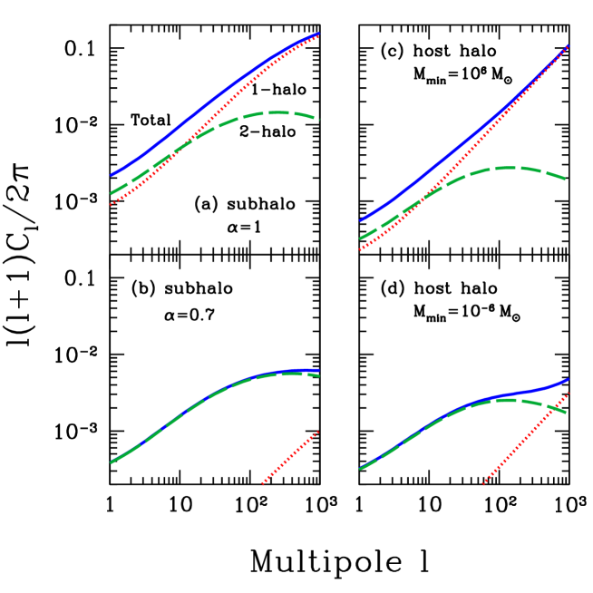
We use these two cases, and 0.7, to bracket the uncertainty in . With , we assume that all the substructures survive the tidal disruption, which is probably a very optimistic approximation. For , on the other hand, we allow some amount of disruption effect, and the angular power spectrum is totally dominated by the 2-halo term, another extreme situation. For even smaller values of , the 1-halo term disappears but the 2-halo term decreases only slightly; thus we do not consider these cases any further.
We also consider the case in which the smooth host halo component dominates the annihilation signal. (I.e., substructures are unimportant.) The gamma-ray emission profile is proportional to the density squared, and this case was in fact carefully studied in AK06. (This case, however, requires additional assumption such that the density profile of the Milky Way is much shallower than NFW, in order not to violate the constraint from the Galactic Center Ando2005 .) The right panels of Fig. 2 show the angular power spectrum of smooth-halo cases with different values of the minimum mass, . Unlike the subhalo-dominated case, the CGB flux is very sensitive to the choice of . This is because the halo concentration is larger for smaller halos Bullock2001 , and the gamma-ray luminosity from each halo is very sensitive to the concentration parameter. We again adopt two extreme cases here, one dominated by 1-halo term and the other by 2-halo term. The shape of the 1-halo term on the right panels is steeper than that on the left panels (subhalo-dominated case), as the signal is more concentrated at the central region. We see below that this tendency converges to when the source is infinitely small as expected for point-like astrophysical sources such as blazars. As for the 2-halo term, the shape is almost the same as the subhalo-dominated case. The normalization, however, is smaller, because the contribution from less massive halos is enhanced when the dark matter distribution is smooth (owing to large concentration of small halos), and less massive halos are less biased.
As a final remark in this section, we discuss the case with other density profiles. Although the NFW profile is most widely used in the literature, our knowledge of the density profile is still far from converged. In particular towards the central region, density might keep rising or converge at some constant value. Therefore, one might question about the impact of the different profiles on the angular power spectrum. We have already seen the tendency such that the steeper the gamma-ray emission profile becomes, the harder the 1-halo term of angular power spectrum gets. Exactly the same argument applies here as well. If the profile has a flat core within some radius, the 1-halo term should be flattened above some that corresponds to the core radius, but this modification at such a small scale will not be detected with GLAST (see discussions about detectability in Sec. V.3). The flattened profile could also be caused by the tidal disruption of subhalos. This means that it controls both the shape (via the profile) and normalization (via the number distribution, or ) of the 1-halo term; but the latter would be much more prominent. On the other hand, the 2-halo term would stay almost the same even if we changed the density profile, thus providing the guaranteed power spectrum that is independent of the density profile adopted.
IV Cosmic gamma-ray background anisotropy II: blazars
IV.1 Formulation
When sources are point-like just as blazars, the angular power spectrum of the CGB is given by
| (18) |
where the first, Poisson term , corresponds to the 1-halo term, and the second, correlation term , to the 2-halo term. The Poisson term represents the shot noise that does not depend on the multipole ’s, while the correlation term is due to the intrinsic spatial correlation of sources. These two terms are related to the spatial power spectrum through
| (19) | |||||
where the lower and upper bounds of integration over and are the same as in Eq. (11). Detailed derivations are given in Appendix A.2. Here the power spectrum of blazars is approximated as , and the blazar bias, , represents how strongly blazars cluster compared with dark matter. (See also Sec. 2.1 of Ref. Ando2006b .)
While the blazar bias, , is currently unknown, it will probably be measured directly from GLAST blazar catalog Ando2006b . (This measurement is, however, limited to the bias of resolved blazars, which can be different from the bias of unresolved blazars which contribute to the CGB anisotropy.) At the moment, one may estimate from several approaches including the angular and spatial correlation analysis of optical quasars Croom2005 ; Myers2006 and X-ray selected AGNs Yang2003 ; Basilakos2005 ; Gandhi2006 . These results, however, are not consistent with each other, potentially due to some observations being biased by a limited field of view covered, or because there is something wrong in our understanding of the unified picture of the AGNs. In any case, a very wide range of the blazar bias is still allowed, ; see Sec. 3.2 of Ref. Ando2006b for a more detailed discussion.
IV.2 Results
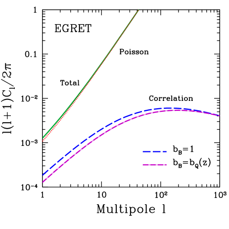
Figure 3 shows the angular power spectrum of the CGB from blazars predicted for EGRET. The dotted lines show the Poisson term [Eq. (19)], the dashed lines show the correlation part [Eq. (LABEL:eq:corr)] evaluated with , and the solid lines show the total. While the blazar bias could perhaps vary from to 5, the Poisson term dominates the angular power spectrum at all multipoles if . The dominance of Poisson term is due to a relatively small number of bright blazars just below EGRET’s sensitivity. The Poisson term will decrease as we remove more fainter objects. We also remark that the does not depend on the gamma-ray energy, since we here assume all the blazars have the power-law spectrum with the same spectral index of , and this energy dependence exactly cancels when we divide by the mean intensity squared to obtain the normalized power spectrum [see Eqs. (19) and (LABEL:eq:corr)].
For GLAST, we choose the point source flux limit of cm-2 s-1 ( MeV), times better than EGRET, which is expected to be achieved after two years of all-sky survey observations of sources with a spectral index of 2 Gehrels1999 . Our predictions for from GLAST data are shown in Fig. 4. As GLAST can detect and remove more fainter objects than EGRET, the Poisson term is greatly reduced while the correlation part is almost unchanged. If the blazar bias is larger than 1, the correlation part would dominate the angular power spectrum at low ’s, which would allow us to measure the average bias of unresolved blazars.
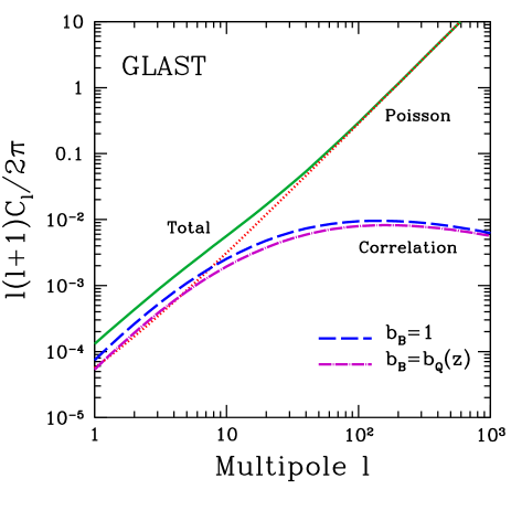
We also show the correlation part of the angular power spectrum using a bias model which was inferred from the optical quasar observations Croom2005 ; Myers2006 :
| (21) |
If the unification picture of the AGNs is correct, then it may be natural to set . The results from this calculation are shown as the dot-dashed curves in Figs. 3 and 4. We find that these results are quite similar to the case of . This is because at low redshift, , the quasar bias is close to 1, and the main contribution to the CGB from blazars comes also from relatively low-redshift range. Once again, we note that the quasar bias [Eq. (21)] is significantly different from the bias inferred from the X-ray AGN observation, which indicated stronger clustering Yang2003 ; Basilakos2005 ; Gandhi2006 . Therefore, one should keep in mind that a wide range of the blazar bias, possibly up to , is still allowed. Hereafter, we adopt as our canonical model, and note that simply scales as .
V Distinguishing dark matter annihilation and blazars
The main goal in this paper is to study how to distinguish CGB anisotropies from dark matter annihilation and from blazars. The current uncertainty in the blazar bias would be the source of systematic errors, but this can be reduced significantly by several approaches, such as the upgraded and converged bias estimations of AGNs from the other wavebands, direct measurement of the blazar bias from the detected point sources by GLAST Ando2006b , and the CGB anisotropy at different energies where the contribution from dark matter annihilation is likely to be small.
V.1 Formulation for the two-component case
The total CGB intensity is the sum of dark matter annihilation and blazars:
| (22) | |||||
| (23) |
where the subscripts and denote blazar and dark matter components, respectively. The expansion coefficients of the spherical harmonics are given by
| (24) | |||||
where , . These and are the fraction of contribution from the blazars and dark matter annihilation to the total CGB flux, and we have the relation . Therefore, is defined as the coefficient of the spherical harmonic expansion if each component is the only constituent of the CGB flux, the same definition as in the previous sections or of AK06. The total angular power spectrum, , is therefore written as
| (25) |
where and are the angular power spectrum of the CGB from blazars (Sec. IV) and dark matter annihilation (Sec. III and AK06), respectively, and is a cross correlation term. This cross correlation term is derived in Appendix B, and is again divided into 1-halo and 2-halo terms, i.e.,
| (26) |
where each term is given by
| (27) | |||||
| (28) | |||||
for the subhalo-dominated annihilation, and
| (29) | |||||
| (30) | |||||
for the host-halo-dominated annihilation; is the Fourier transform of . Here we note that the function in the latter expressions [Eqs. (29) and (30)] is different from Eq. (6), but is given by Eq. (5) of AK06. In order to evaluate the 1-halo term, we need a relation between blazar luminosity and its host mass , for which we use Eq. (22) of Ref. Ando2006b .
V.2 Anisotropy due to dark matter annihilation in the two-component case
Since our main thrust here is how to detect the dark matter annihilation signature out of the CGB in the presence of more common (and plausibly known) blazar component, we focus our attention only on the energy of 10 GeV, a typical energy of gamma rays expected from the annihilation of dark matter particles with a mass of GeV. From now on we treat the blazar contribution as the “background noise.” A signal and background of the angular power spectrum is, respectively,
| (31) | |||||
| (32) |
and we assume that the background is very well known. This is a reasonable assumption, provided that we can model the GLF and bias of unresolved sources from those of resolved (detected) sources in the GLAST data. One can also calibrate the background (blazar) component using the angular power spectrum of the CGB at lower energies such as 100 MeV, where contribution from the dark matter (neutralinos) annihilation may be ignored.
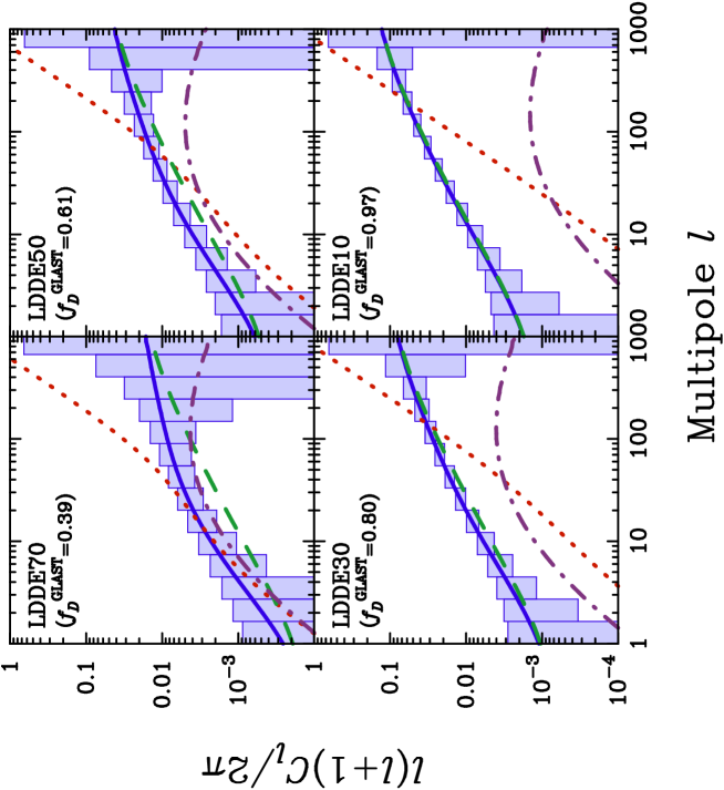
We use several LDDE parameter sets for the blazar GLF, which are listed in Table 1. The faint end of the GLF, which makes the largest contribution to the CGB, is given by , where is the faint-end slope and is the overall normalization Narumoto2006 . We vary these parameters such that the blazars explain a certain fraction, , of the CGB intensity measured by the EGRET at 10 GeV. We call these models LDDE10, LDDE30, LDDE50, and LDDE70 for , 0.3, 0.5, and 0.7, respectively. We note that the best-fitting LDDE model, , explains only % of the CGB flux at 10 GeV, and therefore, one should keep in mind that this list includes models that are somewhat disfavored from the redshift and luminosity distributions of the EGRET blazars. In the two-component treatment, the dark matter fraction is obviously obtained by .
As for the GLAST data, the contribution to the CGB from blazars will be greatly reduced as GLAST can resolve and remove more blazars. On the other hand, the contribution from dark matter annihilation will not change because it is unlikely that we can detect individual dark matter halos via annihilation even with GLAST Oda2005 ; Horiuchi2006 . Therefore, the total CGB intensity, , that would be measured by GLAST would be smaller than that measured by EGRET, while keeping intensity from dark matter annihilation unchanged. The expected fractional contributions to the CGB in the GLAST data from blazars or dark matter annihilation are also shown in Table 1.
| Model | |||||
|---|---|---|---|---|---|
| LDDE10 | 0.1 | 0.9 | 0.03 | 0.97 | |
| LDDE30 | 0.3 | 0.7 | 0.20 | 0.80 | |
| LDDE50 | 0.5 | 0.5 | 0.39 | 0.61 | |
| LDDE70 | 0.7 | 0.3 | 0.61 | 0.39 |
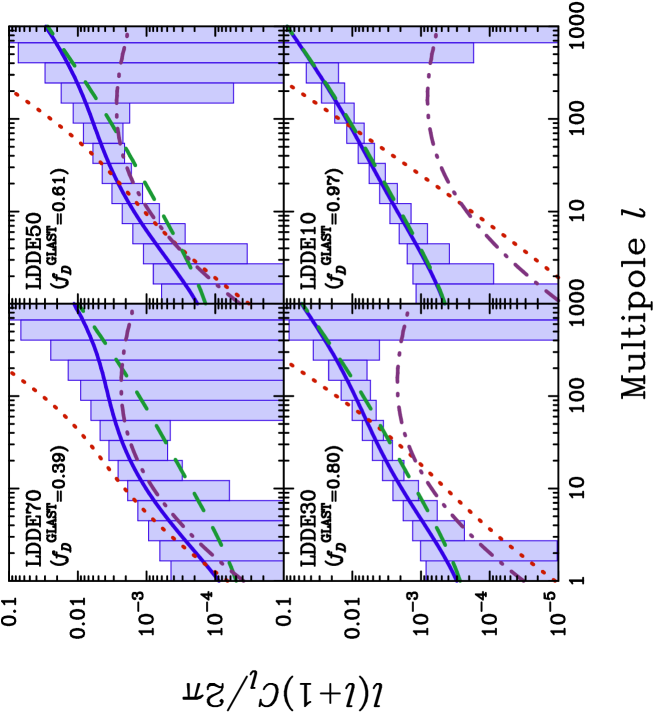
In Figs. 5 and 6, we show the angular power spectrum of dark matter annihilation (i.e., ; solid) as well as of background (; dotted) that would be measured by GLAST, for the blazar models shown in Table 1. We assume that the dark matter signal is dominated by substructures. We also show the expected 1- error bands of . Note that the error bands do include contributions from the blazar power. (See Sec. V.3 for the error estimation.) The subhalo distribution in each halo is assumed to be (Fig. 5) and (Fig. 6). The shape of the angular power spectrum is quite different between dark matter annihilation and blazars, a characteristic that should be useful for a smoking gun detection of dark matter annihilation.
Even though the dark matter contribution to the CGB is relatively small for , the cross correlation term (due mainly to 2-halo term) is still reasonably large; we find that the 1-halo term of the cross correlation is always negligibly small as long as an empirical luminosity–host mass relation is used (Eq. (22) of Ref. Ando2006b ). Although the shape of the cross correlation is similar to the pure blazar correlation term (because both are proportional to the linear power spectrum ), its normalization gives us useful clue of the source because the normalization of the pure blazar term should be known to reasonable accuracy in advance.
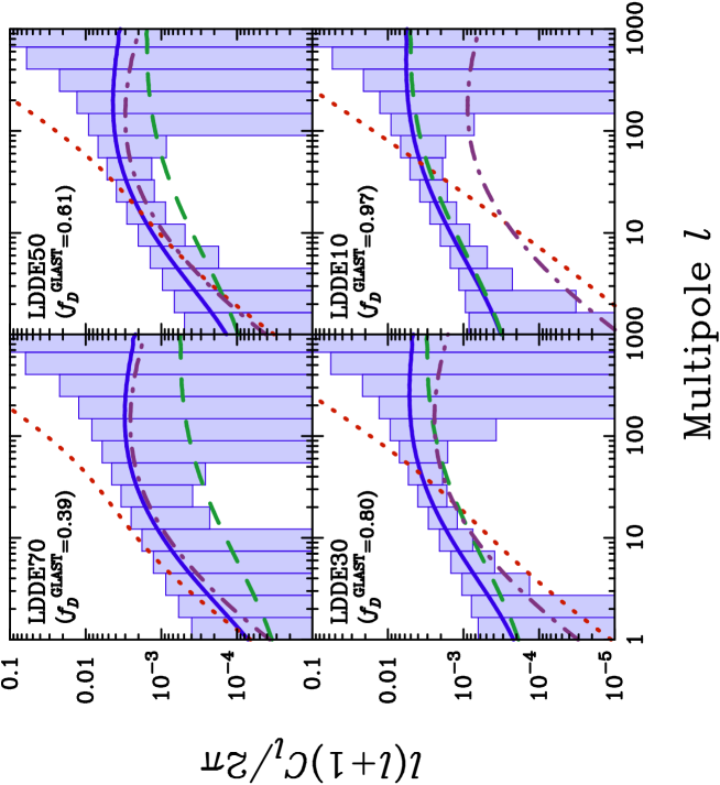
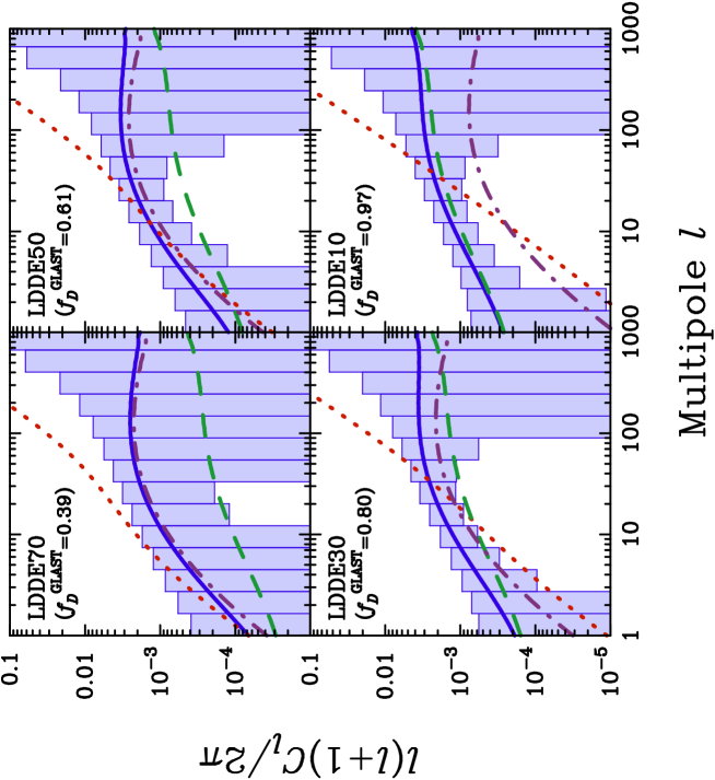
We then repeat the same analysis for the host-halo-dominated annihilation (no substructures). This is a straightforward extension of the study in AK06, to which the background is added. We show in Figs. 7 and 8 the power spectra for and , respectively. The smaller minimum mass is motivated by the free-streaming scale of neutralinos, Green2005 ; Loeb2005 ; Profumo2006 , while the larger one represents an extreme case in which halos smaller than a million solar masses () have been tidally disrupted. (Note, however, that there still remains large allowed range for the former case, – Profumo2006 ). Compared with the subhalo-dominated case, the anisotropy signature is typically smaller, but the general tendency is almost the same, justifying qualitative arguments regarding substructures given in AK06.
V.3 Can GLAST detect dark matter annihilation?
We use the standard procedure to calculate the projected 1- error (binned over ) on the extracted power spectrum of the CGB from dark matter annihilation:
| (33) |
where is the fraction of the sky covered by GLAST, is the bin width (which we shall take to be ), is the power spectrum of photon noise, and and are the photon numbers of the CGB and total (CGB plus other backgrounds), respectively, expected from the region , and is the window function of a Gaussian point spread function, . Note that this formula assumes that CGB anisotropy obeys Gaussian statistics. We take the following specifications for GLAST: the field of view is sr, the angular resolution is , and the effective area is cm2, both evaluated at GeV Gehrels1999 . We assume a two-year all-sky survey ( yr), which corresponds to mean exposure of cm2 s, towards each point in the sky.
Equation (33) clearly shows that the “astrophysical background noise” from blazars, , contributes to the error budget. On the other hand, the background that contributes to includes detector noise and Galactic gamma-ray radiation, which we call foreground. The detector noise is very small for GLAST, about 5% of the CGB flux above 100 MeV; this decreases significantly as the gamma-ray energy and the detector noise is safely assumed to be negligible. The Galactic foreground is more difficult to estimate, but according to recent calculations using a numerical code of the Galactic cosmic-ray propagation, its intensity at 10 GeV is estimated to be at high Galactic latitudes, , which is an order of magnitude smaller than the observed CGB intensity (see Fig. 4 of Ref. Strong2004b ). Below this latitude, the Galactic foreground entirely dominates the gamma-ray flux; thus, we do not consider further. We also note that the Galactic foreground may contribute to the due to spatial fluctuation of the sources, but we neglect this effect in the following arguments. We postulate that this is a reasonable approximation because its flux at the large Galactic latitude is very small compared with the CGB, which suppresses the contribution to the total as well; including this effect requires a detailed modeling of the Galactic cosmic-ray propagation, which is beyond the scope of the present study. The fraction of the sky relevant to our analysis is therefore , which is reasonably close to 1. We do not lose much by this Galactic cut. The number of CGB photons expected from this region and for yr is , while the corresponding photon count from foreground is —negligible compared with that of the CGB. We finally obtain sr. Note that this number is based upon the CGB intensity measured from EGRET, and it will be smaller for GLAST because GLAST can detect and remove more fainter blazars. While this reduction is eventually found to give no significant effect, we take more precise approach in the actual error estimation. Here, just in order to provide a rough idea of the size of each quantity, we used the CGB flux obtained with EGRET.
We show our predictions with the error bars calculated from Eq. (33) in Figs. 5–8. We find that, for any models we have considered here, one should be able to detect the angular power spectrum from dark matter annihilation with GLAST in two years of operation, as long as the dark matter contribution to the mean CGB flux is greater than 30% at some energy within the GLAST energy window. This statement is independent of the density profile adopted as it is derived with the guaranteed power spectrum, the 2-halo term.
VI Discussion and conclusions
In this paper we have presented detailed calculations of the angular power spectrum of CGB anisotropy from dark matter annihilation in cosmological dark matter halos as well as from unresolved blazars. The power spectrum of dark matter annihilation from smooth NFW halos (i.e., no substructures) has been calculated by AK06 Ando2006a , and the power spectrum of resolved (detected) blazars has been calculated by Ref. Ando2006b . Our work builds on and extends these results by taking into account the effects of dark matter substructures explicitly, by means of the Halo Occupation Distribution of subhalos. These calculations should provide a useful benchmark for the angular power spectrum of CGB that would be measured by GLAST.
Our results are very encouraging: one should be able to detect the angular power spectrum from dark matter annihilation with GLAST, whether dark matter halos are smooth or clumpy, as long as the dark matter contribution to the mean CGB flux is greater than 30% at some energy within the GLAST energy window. This is a rather modest requirement given the fact that unresolved blazars appear to contribute to the mean CGB only at the 25–50% level Narumoto2006 . As far as the mean CGB is concerned it has been pointed out that subhalos are necessary in order for dark matter annihilation to make a significant contribution without violating stringent constraints from the Galactic Center Ando2005 ; Oda2005 ; Horiuchi2006 . Thus, our current “best” predictions are either Fig. 5 or Fig. 6, depending on the degree to which tidal disruption of subhalos is important.
The “background noise” for dark matter annihilation searches includes the blazar anisotropy, detector noise, and the Galactic foreground. The blazar anisotropy should be well calibrated with the CGB anisotropy at lower energies (where dark matter signal is probably unimportant), analysis of AGNs selected with other wavebands, and/or the power spectrum of resolved point sources. The detector noise is always negligible. The Galactic foreground contamination is serious near the plane, , whereas its flux is found to be at most % of the CGB flux at high Galactic latitudes. The anisotropy due to the foreground is thus accordingly reduced. We also note that dark matter annihilation in the Galactic halo may also give a contribution to the CGB flux comparable to that from the cosmological halos (e.g., Ref. Oda2005 ; Diemand2006 ). Adding this component would increase the predicted anisotropy from dark matter annihilation.
GLAST covers energy spectrum up to 300 GeV, which might enable us to probe a line signature in the CGB due to direct annihilation of dark matter particles into two photons (or one photon plus one boson). In addition to quite robust spectral feature, one could also use the CGB anisotropy as a consistency check. When the spectrum has a feature as the case of lines, the angular power spectrum becomes larger Zhang2004 ; Ando2005 , which makes this method even more promising.
Finally, we comment on how our conclusions might be affected by the other astrophysical sources (of either known or unknown species) that we have not considered. If the gamma-ray emitter is a point source and follows the distribution of dark matter halos, then the number of such sources contributing to the CGB is the only parameter that determines the amplitude of the power spectrum. Whatever the sources are, they should be dimmer than blazars on average; we must have seen them in the EGRET data otherwise. If the number of such sources is much larger than blazars, then the Poisson term, , is highly suppressed and is unimportant. If these sources are rare, forming only in large halos, the power spectrum (both 1-halo and 2-halo terms) can be large, but it is extremely difficult for them to give a dominant contribution to the CGB.
If these sources are spatially extended, e.g., clusters of galaxies, then the shape of the angular power spectrum depends on their gamma-ray profile. How the galaxy clusters are extended in gamma rays depends on the emission mechanism, which is uncertain. (No direct detection of gamma rays towards known clusters has been made so far.) Incidentally one can make the most conservative (or pessimistic) prediction as to how much the unresolved clusters would contribute to CGB anisotropy, by assuming that the galaxy clusters are point sources. We have performed the same calculations for galaxy clusters for both the proton-proton collision Colafrancesco1998 and inverse-Compton models Totani2000 . Our results again suggest that the dark matter component should be detectable significantly, as long as its contribution to the EGRET CGB is more than %. Angular distribution of background radiation from galaxy clusters has been investigated also in previous papers, for radio waveband Waxman2000 ; Keshet2004 as well as for gamma rays Waxman2000 ; Keshet2003 .
Based upon these results, we conclude that anisotropy in the CGB that would be measured by GLAST has to be analyzed in search for signatures of dark matter annihilation. If detected, it should provide us with the first (albeit indirect) evidence for emission from dark matter particles, which would shed light on the nature of the still-mysterious dark matter in the universe.
Acknowledgements.
S.A. and E.K. would like to thank Jennifer Carson for useful discussions. S.A. is also grateful to Edward Baltz, Marc Kamionkowski, Stefano Profumo, and Lawrence Wai for comments. S.A. was supported by Sherman Fairchild Foundation at Caltech. E.K. acknowledges support from the Alfred P. Sloan Foundation. T.N. and T.T. were supported by a Grant-in-Aid for the 21st Century COE “Center for Diversity and Universality in Physics” from the Ministry of Education, Culture, Sports, Science and Technology of Japan.Appendix A Relation between angular and spatial power spectrum
A.1 Dark matter substructure
In this subsection, we derive Eq. (14) following the halo model approach Scherrer1991 ; Seljak2000 . Since the gamma-ray intensity due to annihilation dominated by subhalos depends on the density, which can be written as a superposition of densities in different halos, we obtain the following expression for the volume emissivity:
| (34) | |||||
where is the -dimensional delta function, and represents comoving coordinate. As in Ref. Scherrer1991 , the ensemble average of the sum over delta functions is simply the seed density:
| (35) |
and using this into Eqs. (34) and (1), we recovers Eq. (5) since .
We then define the two-point correlation function of subhalos as
| (36) |
where . Now we evaluate . The ensemble average of the product of seed densities is written as follows Scherrer1991 :
| (37) | |||||
where is the -point correlation function of the seed. The first term represents the two-halo contribution, i.e., two points considered, and , are in two distinct halos, while the second are the one-halo contribution where these two points are in the same halo. By substituting this expression into Eq. (34), and using the relation and Eq. (2), we obtain
We define the power spectrum of subhalos as Fourier transforms of . Remembering that convolution in the real space corresponds to a simple product in the Fourier space, we obtain for the expression for as follows:
| (40) | |||||
where we used an approximation as by introducing the bias factor and linear matter correlation function . These expressions are identical to Eqs. (LABEL:eq:1-halo_term) and (17).
Finally we derive the relation between angular power spectrum and spatial power spectrum in the following. We start with the angular correlation function that is defined by
| (41) |
where . Using this definition together with Eqs. (1), (2), (6), and (36), we get
| (42) |
where and are redshifts corresponding to and , respectively, and we suppressed energy indices for simplicity. To further simplify, we use small separation approximation following Ref. Peebles1980 [we use , with definitions of ], and arrive at
| (43) |
The angular power spectrum is related to the correlation function through
| (44) |
for small scales, or for large multipoles. Then, the Fourier transformation of the relevant quantity simplifies as follows:
| (45) | |||||
In the second equality, we decomposed the wavenumber by the components parallel and perpendicular to , i.e., , and used . Therefore, together with Eqs. (43) and (44), we arrive at our demanded relation, Eq. (14).
A.2 Blazars
In this subsection, we derive Eqs. (19) and (LABEL:eq:corr) following discussions in Ref. Peebles1980 (see also, Ref. Komatsu1999 ). The Poisson noise is obtained by setting for [Eq. (41)], and it is given by Eq. (58.14) of Ref. Peebles1980 [note with Eq. (58.12) that the definition of the angular power spectrum is slightly different], which is
in our notation. It is equivalent to Eq. (19).
The correlation term of the angular power spectrum , on the other hand, is obtained with the Fourier transformation of the angular correlation function for (Eq. (58.6) of Ref. Peebles1980 )
where is the two-point correlation function of blazars; here we suppressed the luminosity index but note that this dependence should appear in general. Then, using the Fourier transformation that is similar to Eq. (45), we obtain the correlation part of the angular power as
where in the last equality we used the relation and Eq. (9). This is very similar to Eq. (LABEL:eq:corr). It is obvious that if we introduced the bias parameter from the beginning, as , then we would have obtained exactly the same result as Eq. (LABEL:eq:corr).
Appendix B Cross correlation between dark matter annihilation and blazars
We here derive the formulation for the angular cross correlation between blazars and dark matter annihilation, , in the subhalo-dominated case, Eqs. (27) and (28), and in the host-halo-dominated case, Eqs. (29) and (30), respectively in the following subsections. Once again, we follow the halo model approach highlighted in Refs. Scherrer1991 ; Seljak2000 .
B.1 Subhalo-dominated case
B.2 Host-halo-dominated case
In the case of host-halo-dominated annihilation, the intensity is proportional to density squared:
where is the overdensity. Therefore, we need to evaluate the ensemble average of the product of seed densities as follows:
| (51) | |||||
The first term represents the three-halo contribution, i.e., three points considered , and are in three different halos; the second to fourth terms are the two-halo contribution, where two points are in one halo and the rest one point is in the other halo; the last term shows the one-halo contribution, where all three points are in the same halo. Now, our particular focus here is that one point, say , represents the blazar position, while the other two, and , the place of the dark matter annihilation. Since the latter effect is proportional to the density squared at one point, we have . In this case, considering the fact that the halos are spatially exclusive, one can omit terms except for the second (2-halo term) and the last (1-halo term).
We then evaluate the one-halo and two-halo terms. By substituting the above expression, we get
| (52) | |||||
| (53) | |||||
where we used Eq. (6) of AK06 to reach in the second expression. We again use small separation approximation, , and get
| (54) | |||||
To obtain the angular power spectrum, we Fourier-transform this expression. Using the similar relations to Eq. (45), we finally arrive at Eqs. (29) and (30).
References
- (1) P. Sreekumar et al., Astrophys. J. 494, 523 (1998).
- (2) A. W. Strong, I. V. Moskalenko and O. Reimer, Astrophys. J. 613, 956 (2004).
- Padovani et al. (1993) P. Padovani, G. Ghisellini, A. C. Fabian and A. Celotti, Mon. Not. R. Astron. Soc. 260, L21 (1993).
- (4) F. W. Stecker, M. H. Salamon and M. A. Malkan, Astrophys. J. 410, L71 (1993).
- (5) M. H. Salamon and F. W. Stecker, Astrophys. J. 430, L21 (1994).
- Chiang et al. (1995) J. Chiang, C. E. Fichtel, C. von Montigny, P. L. Nolan and V. Petrosian, Astrophys. J. 452, 156 (1995).
- (7) F. W. Stecker and M. H. Salamon, Astrophys. J. 464, 600 (1996).
- Chiang & Mukherjee (1998) J. Chiang and R. Mukherjee, Astrophys. J. 496, 752 (1998).
- Mücke & Pohl (2000) A. Mücke and M. Pohl, Mon. Not. R. Astron. Soc. 312, 177 (2000).
- (10) T. Narumoto and T. Totani, Astrophys. J. 643, 81 (2006).
- (11) P. Giommi, S. Colafrancesco, E. Cavazzuti, M. Perri and C. Pittori, Astron. Astrophys. 445, 843 (2006).
- (12) C. D. Dermer, astro-ph/0605402.
- (13) V. S. Berezinsky, P. Blasi and V. S. Ptuskin, Astrophys. J. 487, 529 (1997).
- (14) S. Colafrancesco and P. Blasi, Astropart. Phys. 9, 227 (1998).
- (15) C. Pfrommer and T. A. Ensslin, Astron. Astrophys. 413, 17 (2004); 426, 777(E) (2004).
- (16) A. Loeb and E. Waxman, Nature 405, 156 (2000).
- (17) T. Totani and T. Kitayama, Astrophys. J. 545, 572 (2000).
- (18) E. Waxman and A. Loeb, Astrophys. J. 545, L11 (2000).
- (19) U. Keshet, E. Waxman, A. Loeb, V. Springel and L. Hernquist, Astrophys. J. 585, 128 (2003).
- (20) F. Miniati, Mon. Not. R. Astron. Soc. 342, 1009 (2003).
- (21) S. Gabici and P. Blasi, Astrophys. J. 583, 695 (2003).
- (22) S. Gabici and P. Blasi, Astropart. Phys. 19, 679 (2003).
- (23) S. Gabici and P. Blasi, Astropart. Phys. 20, 579 (2004).
- (24) O. Reimer, M. Pohl, P. Sreekumar and J. R. Mattox, Astrophys. J. 588, 155 (2003).
- (25) W. Kawasaki and T. Totani, Astrophys. J. 576, 679 (2002).
- (26) C. A. Scharf and R. Mukherjee, Astrophys. J. 580, 154 (2002).
- (27) G. Jungman, M. Kamionkowski and K. Griest, Phys. Rep. 267, 195 (1996).
- (28) L. Bergström, Rep. Prog. Phys. 63, 793 (2000).
- (29) G. Bertone, D. Hooper and J. Silk, Phys. Rep. 405, 279 (2005)
- (30) L. Bergström, J. Edsjö and P. Ullio, Phys. Rev. Lett. 87, 251301 (2001).
- (31) P. Ullio, L. Bergström, J. Edsjö and C. G. Lacey, Phys. Rev. D 66, 123502 (2002).
- (32) J. E. Taylor and J. Silk, Mon. Not. R. Astron. Soc. 339, 505 (2003).
- (33) K. Ahn and E. Komatsu, Phys. Rev. D 71, 021303(R) (2005).
- (34) K. Ahn and E. Komatsu, Phys. Rev. D 72, 061301(R) (2005).
- (35) T. Oda, T. Totani and M. Nagashima, Astrophys. J. 633, L65 (2005).
- (36) S. Horiuchi and S. Ando, Phys. Rev. D 74, 103504 (2006).
- (37) G. Bertone, A. R. Zentner and J. Silk, Phys. Rev. D 72, 103517 (2005).
- (38) G. Bertone, Phys. Rev. D 73, 103519 (2006).
- (39) S. Ando, Phys. Rev. Lett. 94, 171303 (2005).
- (40) D. Elsässer and K. Mannheim, Phys. Rev. Lett. 94, 171302 (2005).
- (41) S. Ando and E. Komatsu, Phys. Rev. D 73, 023521 (2006) [AK06].
- (42) J. F. Navarro, C. S. Frenk and S. D. M. White, Astrophys. J. 462, 563 (1996).
- (43) J. F. Navarro, C. S. Frenk and S. D. M. White, Astrophys. J. 490, 493 (1997).
- (44) J. S. Bullock et al., Mon. Not. R. Astron. Soc. 321, 559 (2001).
- (45) R. K. Sheth and G. Tormen, Mon. Not. R. Astron. Soc. 308, 119 (1999).
- (46) S. Ando, E. Komatsu, T. Narumoto and T. Totani, Mon. Not. R. Astron. Soc. (2007), in press [astro-ph/0610155].
- (47) D. J. Thompson et al., Astrophys. J. Suppl. Ser. 86, 629 (1993)
- (48) U. Keshet, E. Waxman and A. Loeb, JCAP 0404, 006 (2004).
- (49) D. J. Eisenstein and W. Hu, Astrophys. J. 511, 5 (1997).
- (50) H. J. Mo and S. D. M. White, Mon. Not. R. Astron. Soc. 282, 347 (1996).
- (51) S. M. Croom et al., Mon. Not. R. Astron. Soc. 356, 415 (2005).
- (52) A. D. Myers et al., Astrophys. J. 638, 622 (2006).
- (53) Y. X. Yang, R. F. Mushotzky, A. J. Barger, L. L. Cowie, D. B. Sanders and A. T. Steffen, Astrophys. J. 585, L85 (2003).
- (54) S. Basilakos, M. Plionis, A. Georgakakis and I. Georgantopoulos, Mon. Not. R. Astron. Soc. 356, 183 (2005).
- (55) P. Gandhi et al., astro-ph/0607135.
- (56) N. Gehrels and P. Michelson, Astropart. Phys. 11, 277 (1999).
- (57) A. M. Green, S. Hofmann and D. J. Schwarz, JCAP 0508, 003 (2005).
- (58) A. Loeb and M. Zaldarriaga, Phys. Rev. D 71, 103520 (2005).
- (59) S. Profumo, K. Sigurdson and M. Kamionkowski, Phys. Rev. Lett. 97, 031301 (2006).
- (60) A. W. Strong, I. V. Moskalenko and O. Reimer, Astrophys. J. 613, 962 (2004).
- (61) J. Diemand, M. Kuhlen and P. Madau, astro-ph/0611370.
- (62) P. J. Zhang and J. F. Beacom, Astrophys. J. 614, 37 (2004).
- (63) U. Keshet, E. Waxman and A. Loeb, Astrophys. J. 617, 281 (2004).
- (64) R. J. Scherrer and E. Bertschinger, Astrophys. J. 381, 349 (1991).
- (65) U. Seljak, Mon. Not. R. Astron. Soc. 318, 203 (2000).
- (66) P. J. E. Peebles, The Large-Scale Structure of the Universe (Princeton University Press, 1980).
- (67) E. Komatsu and T. Kitayama, Astrophys. J. 526, L1 (1999).